ABSTRACT
CHAUDHARY, MANDAR SANJAY. Methods for Learning and Predicting Causal Relationships from Observational Data. (Under the direction of Dr. Nagiza F. Samatova).
Discovering causal relationships from observational data has contributed significantly towards understanding mechanisms of complex systems. Specifically, the domains of biology and climate
science have benefited from observational studies where performing external interventions is
infeasible or impractical. For example, in biology identifying genes having a causal effect on a phenotype (such as riboflavin production rate) has led to prioritizing gene knock-out experiments.
However, the increasing amount of observational data is accompanied by its own set of challenges
such as high-dimensionality, smaller sample size and missing ground truth to validate causal relationships. Thus, developing algorithms that effectively discover causal relationships becomes a
challenging task.
In this dissertation, we propose two main contributions for extracting causal information from observational data. First, in contrast to existing causal feature selection methods, we identify
mean-ingful predictive features by incorporating the causal structure as well as the strength of causal
effects. This leads to discovering relationships that cannot be detected by causal structure learning methods, especially while dealing with high-dimensional data sets with smaller sample size. Second,
we mine observational data to discover patterns of association between variables that discriminate
causal relationships from non-causal relationships. This results in a significant improvement in the quality of output causal relationships.
Traditional causal discovery methods focus on learning the causal structure of a network. The
potential causal relationships in the network are studied by domain scientists to validate their hypotheses. Studying each causal relationship can become infeasible in high-dimensional settings.
In the first part of this dissertation, we develop an algorithm to reduce the search space of causal
relationships and evaluate the predictive ability of the factors in such relationships with respect to a given phenomenon of interest such as seasonal rainfall in a geographic region. Results show that
our algorithm is consistently among the top performing methods compared to state-of-art feature
selection methods. Additionally, our algorithm identifies physically interpretable features that can explain the prediction performance of the model.
In the second part, we develop a graph partitioning based approach to complement a constraint-based causal structure learning algorithm. Partitioning a graph into smaller subgraphs guides the
process of discovering causal relationships. Consequently, reducing the error of falsely removing a
causal relationship. Experiments on networks of different sizes, complexities and data types show the effectiveness of our algorithm.
can be transformed into a supervised learning problem. We develop an algorithm that utilizes kernel
mean embedding to generate patterns from a parent-child and a non-parent child relationship. Simulations show the presence of a discriminative pattern in networks generated with non-linear
data. Experiments on synthetic data and real-world data illustrate the effectiveness of our algorithm
© Copyright 2019 by Mandar Sanjay Chaudhary
Methods for Learning and Predicting Causal Relationships from Observational Data
by
Mandar Sanjay Chaudhary
A dissertation submitted to the Graduate Faculty of North Carolina State University
in partial fulfillment of the requirements for the Degree of
Doctor of Philosophy
Computer Science
Raleigh, North Carolina
2019
APPROVED BY:
Dr. Dennis R. Bahler Dr. Steffen Heber
Dr. R. Raju Vatsavai Dr. Nagiza F. Samatova
DEDICATION
BIOGRAPHY
Mandar Chaudhary is a PhD student in the department of Computer Science at the North Carolina State University advised by Dr. Nagiza F. Samatova. He received his M.S. in Computer Science
from North Carolina State University in 2014 and a B.E. in Computer Engineering from Gujarat
Technological University, India in 2012. During his doctoral study, Mandar had appointments as a research assistant and a teaching assistant. He also had the opportunity to work as a data science
ACKNOWLEDGEMENTS
My journey as a PhD student would not have been possible without the constant support and guidance from a number of people. First, I would like to thank my advisor Dr. Nagiza F. Samatova
for her continued support and guidance during my doctoral studies. Her wisdom, advice and
encouragement have enabled me to become the person and researcher I am today.
I would like to express my gratitude towards the faculty at the Computer Science department of
North Carolina State University. Particularly, I’m thankful to Dr. Dennis Bahler, Dr. Steffen Heber and Dr. R. Raju Vatsavai for their participation in my advisory committee and for providing insightful
discussions to improve my dissertation. I would also like to thank Dr. George N. Rouskas, Director
of Graduate Programs for his support during my graduate studies.
I was also fortunate to have valuable collaborations from different research institutions. I would
like to thank my collaborators from the National Science Foundation (NSF) Expeditions in
Comput-ing project "UnderstandComput-ing Climate Change: A Data Driven Approach," particularly Dr. Fredrick H. M. Semazzi at North Carolina State University’s Department of Marine, Earth, and Atmospheric
Sciences (MEAS) and Dr. Vipin Kumar at the University of Minnesota. I would also like to thank Dr.
Semazzi’s research group member Michael Angus for his valuable insights regarding the application of my work to climate science domain in Chapter 2. I would also like to thank Dr. Murali Doraiswamy
and Dr. Elizabeth Cirulli at Duke University for their insightful feedback about the application of my
work in biology domain.
Additionally, I am grateful for having the opportunity to work with fellow students and
col-leagues at Dr. Samatova’s research lab. I would like to thank Gonzalo Bello, Steve Harenberg, Stephen
Ranshous, Shiou "Claude" Tian Hsu, Dhara Desai, Changsung Moon, Khelan Patel, Ameeta Muralid-haran, Doel Gonzalez, and David "Drew" Boyuka.
Finally, I am eternally grateful to my family, particularly my parents, Sanjay and Sunita, my
grand-parents, Paruben and Raghuveerbhai, my sister Anuradha and my wife Foram for their unconditional love, motivation and support throughout this journey.
This dissertation is based upon work supported in part by the Laboratory for Analytic Sciences
(LAS) and the NSF grant 1029711. Any opinions, findings, conclusions, or recommendations ex-pressed in this dissertation are those of the author and do not necessarily reflect the views of any
TABLE OF CONTENTS
LIST OF TABLES . . . vii
LIST OF FIGURES. . . ix
Chapter 1 Introduction. . . 1
1.1 Causal Discovery Methods . . . 3
1.1.1 Causal Structure Learning . . . 4
1.1.2 Causal Effect Estimation . . . 5
1.2 Methods for Learning and Predicting Causal Relationships . . . 6
1.2.1 Causality-Guided Feature Selection . . . 7
1.2.2 Graph Partitioning based Causal Discovery . . . 7
1.2.3 Causal Relationship Prediction with Additive Noise Models . . . 8
Chapter 2 Causality-Guided Feature Selection . . . 9
2.1 Introduction . . . 9
2.2 Problem Statement . . . 11
2.3 Method . . . 12
2.3.1 Constructing Causal Graphs and Selecting Potential Causal Relationships . . . 12
2.3.2 Estimating Causal Effects and Assessing its Statistical Significance . . . 15
2.3.3 Feature Selection via Clustering . . . 18
2.4 Empirical Evaluation . . . 18
2.4.1 Data Description . . . 18
2.4.2 Data Preprocessing . . . 20
2.4.3 Temporal Constraints . . . 20
2.4.4 Performance Comparison . . . 21
2.4.5 Additional Experiments . . . 26
2.4.6 Physical Interpretability . . . 27
2.4.7 Time Complexity . . . 29
2.5 Related Work . . . 31
2.6 Conclusion . . . 33
Chapter 3 Graph Partitioning Based Causal Discovery . . . 35
3.1 Introduction . . . 35
3.2 Related Work . . . 36
3.3 Preliminaries . . . 37
3.4 Method . . . 38
3.4.1 Constructing Undirected Weighted Independence Graphs . . . 39
3.4.2 Community-driven Causal Discovery (CDCD) . . . 40
3.4.3 PC algorithm . . . 46
3.5 Empirical Evaluation . . . 46
3.5.1 Results . . . 48
3.5.2 Time Complexity Analysis . . . 50
Chapter 4 Causal Relationship Prediction with Additive Noise Models. . . 52
4.1 Introduction . . . 52
4.2 Preliminaries . . . 53
4.3 Related work . . . 55
4.4 Method . . . 55
4.4.1 Data partition for building regression models . . . 56
4.4.2 Feature creation with kernel mean embeddings . . . 57
4.5 Simulations . . . 60
4.5.1 Synthetic Data . . . 60
4.6 Conclusions and future work . . . 67
Chapter 5 Conclusion. . . 69
5.1 Future Work . . . 70
LIST OF TABLES
Table 2.1 Climate Indices constructed from Reanalysis data to include local variability. . 20 Table 2.2 RMSE scores for prediction of seasonal rainfall at African Sahel (ASR) and East
Africa (EAR), riboflavin production rate (RPR) and cognitive score for male (CS_M) and female (CS_F) patients obtained from all the feature selection methods. RMSE scores within 6% of the best performing method are high-lighted in bold. (∗) indicates that a feature selection method could not find any feature from some of the training sets during cross-validation . . . 22 Table 2.3 A summary of the performance of all the feature selection methods in terms
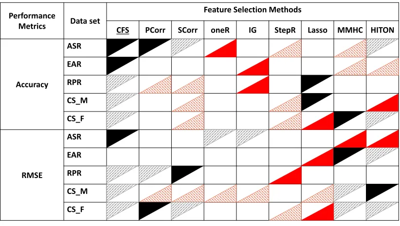
of classification accuracy and RMSE scores across all five data sets. A solid upper triangle indicates the best performing method, whereas a solid lower triangle indicates the worst performing method on a given data set. An upper triangle with pattern indicates that a method’s performance was within 6% of the accuracy and RMSE score of the best performing method, and a lower triangle with pattern indicates a method’s performance was within 6% of the accuracy and RMSE score of the worst performing method. . . 24 Table 2.4 Confidence interval of classification accuracy for prediction of seasonal
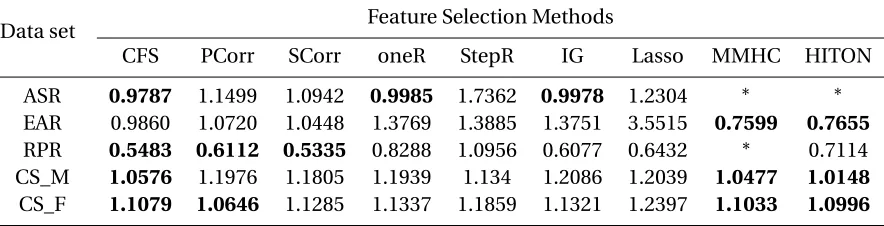
rain-fall at African Sahel (ASR) and East Africa (EAR), riboflavin production rate (RPR) and cognitive score for male (CS_M) and female (CS_F) patients ob-tained from all the feature selection methods. A threshold of 95% was used to measure the confidence intervals. A value highlighted in bold indicates the best performance in terms of classification accuracy on a given dataset and a value underlined indicates the smallest confidence interval width. . . 25 Table 2.5 Confidence interval of root mean squared errors (RMSE) for prediction of
seasonal rainfall at African Sahel (ASR) and East Africa (EAR), riboflavin pro-duction rate (RPR) and cognitive score for male (CS_M) and female (CS_F) patients obtained from all the feature selection methods. A threshold of 95% was used to measure the confidence intervals. A (∗) indicates that RMSE value for a given method was not computed as it failed to select any features in at least one of the cross-validation folds. A value highlighted in bold indicates the best performance in terms of RMSE on a given dataset and a value underlined indicates the smallest confidence interval width. . . 25 Table 2.6 Mean classification accuracy and RMSE scores over leave-one-out cross-validation
for the African Sahel (ASR), East African (EAR), riboflavin production rate (RPR), and cognitive score for male (CS_M) and female (CS_F) patients obtained us-ing MMHC and MMHC+CFS as feature selection methods. A∗indicates that MMHC did not select any feature in at least one of the cross-validation folds. . 26 Table 2.7 A list of ground truth containing the prominent predictive season of the climate
Table 2.8 A list of ground truth containing prominent predictive seasons of the climate indices and their prominent season predicted by our method for the East African region. A - indicates that our method did not find the corresponding climate index as a feature. The months are represented as, 1=Jan, 2=Feb, ..., 9=Sep. . . 31 Table 2.9 A list of frequently selected causal relationships identified by our methodology
along with its frequency count for African Sahel region. . . 32 Table 2.10 A list of frequently selected causal relationships identified by our methodology
along with its frequency count for East African region. . . 33
Table 3.1 A list of different networks and data types used in our experiments. Discrete data sets were generated from five discrete bayesian networks and continuous data sets were generated from two gaussian bayesian networks. . . 47
Table 4.1 Performance metrics for Linear Structural Equation Models on sparse causal graphs,pc o n=2/(p−1). The reported metric is its mean value over 20 simula-tions. The best performance is highlighted. . . 61 Table 4.2 Performance metrics for Nonlinear Structural Equation Models on sparse
causal graphs,pc o n=2/(p−1). The reported metric is its mean value over 20 simulations. The best performance is highlighted. . . 62 Table 4.3 Performance metrics for Nonlinear Structural Equation Models on dense
causal graphs,pc o n = 2∗2/(p−1). The reported metric is its mean value over 20 simulations. The best performance is highlighted. . . 63 Table 4.4 Performance metrics for real-world protein network. The reported metric is
LIST OF FIGURES
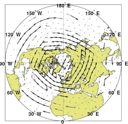
Figure 1.1 An example graph represents information flow for an atmospheric field such as geopotential height around the globe. The nodes (dots) represent spatial points that provide time series data and the directed edges represent the strongest causal relationships between the different values of geopotential height[EUD14]. . . 2 Figure 1.2 The local causal structure of a target variable T consists of its direct causes
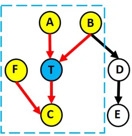
(A, B), direct effects (C) and spouses (F). This structure is referred to as the Markov Blanket of T. Conditioned on its Markov Blanket, T is independent of the remaining variables (D, E)[Ali10a]. . . 3 Figure 1.3 An overview of causal discovery methods categorized based on their
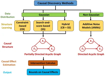
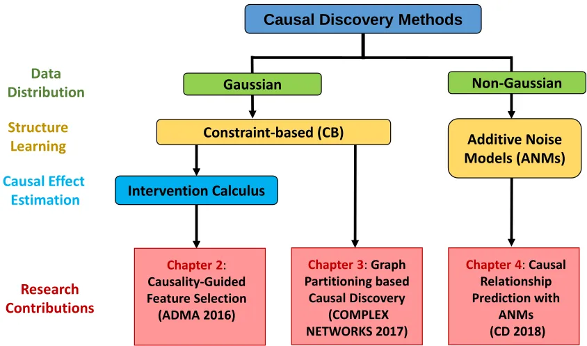
assump-tions about the joint distribution in the observational data. Constraint-based , search-and-score based, hybrid, and causal effect estimation methods as-sume multivariate Gaussian distribution and estimate a partially directed acyclic graph (PDAG). The PDAG can be used to estimate bounds on the causal effects using the so-called intervention calculus. On the other hand, by relaxing the assumption of Gaussianity in the observational data, additive noise models can estimate the complete directed acyclic graph (DAG). . . 4 Figure 1.4 An overview of the dissertation chapters highlighting our contributions to
the research objectives of effective causal discovery. . . 6
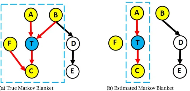
Figure 2.1 2.1a The Markov Blanket of a target variable T consists of its direct causes (A, B), direct effects (C) and spouses (F). T is independent of other variable given its Markov Blanket[Ali10a]. 2.1b An estimated Markov Blanket might be incomplete due to errors made by statistical tests, thereby providing subopti-mal prediction performance. In this case, the edges B→T and F→C were erroneously removed thereby excluding them from the Markov Blanket . . . . 10 Figure 2.2 A completed partially directed acyclic graph (CPDAG) over a set of variables
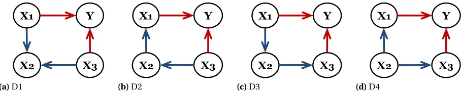
X ={X1,X2,X3,Y}comprising of two directed edges,X1→Y andX3→Y, one undirected edgeX1−X2and one bi-directed edgeX2↔X3. . . 16 Figure 2.3 Figures (a)-(d) represent the set of possible DAGs D1-D4. D1 is an invalid DAG
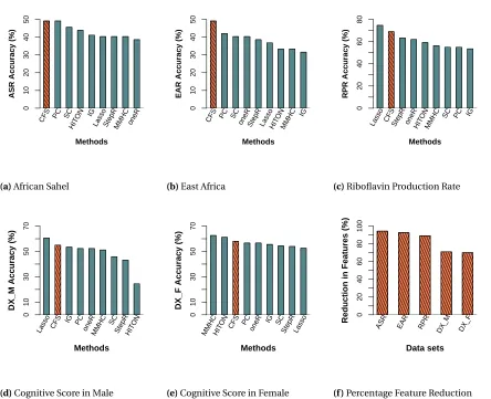
as it contains an additionalv-structure,X1→X2←X3, that is not present in the estimated CPDAG. D2-D4 are valid DAGs and they belong to the same Markov equivalence class. . . 16 Figure 2.4 Mean classification accuracy over leave-one-out cross validation (Accuracy)
Figure 2.5 A summary graph representing frequently selected causal relationships with both climate indices in a relationship having a statistically significant causal effect on the seasonal rainfall in the African Sahel region. A directed edge represents a causal relationship between climate indices in the same month or different months. A self-loop indicates a causal relationship between the same climate index in different months. A dotted line between a climate index and seasonal rainfall indicates the climate index has a statistically significant causal effect on the seasonal rainfall. Figure 2.5a shows the frequently se-lected features and the causal relationships between them. Figure 2.5b shows the frequently selected features by existing state-of-art local causal feature selection methods namely HITON and MMHC. . . 30 Figure 2.6 A summary graph representing frequently selected causal relationships with
both climate indices in a relationship having a statistically significant causal effect on the seasonal rainfall in the East African region. A directed edge represents a causal relationship between climate indices in the same month or different months. A self-loop indicates a causal relationship between the same climate index in different months.Figure 2.6a shows the frequently selected features and the causal relationships between them. Figure 2.6b shows the frequently selected features by existing state-of-art local causal feature selection methods namely HITON and MMHC. . . 30
Figure 3.1 Sample output of community detection on an undirected weighted indepen-dence graph, after removing edges using zero- and first-order CI tests[WB06]. Variables in the same community share the same color. The inter-community variables,Z={3, 4, 8, 10, 15, 17, 18, 19}, serve as the potential d-separators that separate variables in their communities from the rest of the network. . . 41 Figure 3.2 SubgraphsG1andG2are output from the split phase and they are to be merged
to build the full skeleton. Variables in the same community are represented in the same color. Note that in subgraphG1the edge 1−5 is removed whereas inG2the edge is still present. Therefore, in the final merged graph, the edge 1−5 is removed since it is likely that the two variables are d-separated by the variables inG1. . . 44 Figure 3.3 Comparison of the CDCD, PC, and PC-stable algorithms in terms of Structural
Hamming Distance (SHD), True Discovery Rate (TDR), True Positive Rate (TPR), False Positive Rate (FPR) and the standard accuracy metric,d, across five discrete Bayesian Networks and three sample sizes. The reported metric for each network is its mean value from 10 randomly generated data sets. . . . 49 Figure 3.4 Comparison of the CDCD, PC, and PC-stable algorithms in terms of Structural
Figure 4.1 The mean and standard deviation values of features generated from the true parents (see Equation 4.8) (1:300), mix-parents (301:600), and non-parents (601:900) for all the child variables in the training set withp=10 andn=100 for linear SEMs. The first hundred features in a variable set represent the embedding of the regressor set, the next hundred represent the embedding of residuals and the last hundred represent the embedding of both. The true-parent set (pink) and the mix true-parent set (green) are assigned the same class label and the non-parent set (blue) is assigned a different class label. . . 64 Figure 4.2 The mean and standard deviation values of features generated from the true
parents (see Equation 4.8) (1:300), mix-parents (301:600), and non-parents for all the child variables in the training set withp = 10 andn =100 for nonlinear SEMs. The first hundred features in a variable set represent the embedding of the regressor set, the next hundred represent the embedding of residuals and the last hundred represent embedding of both. The true-parent set (pink) and the mix parent set (green) are assigned the same class label and the non-parent set (blue) is assigned a different class label. . . 65 Figure 4.3 The importance of features in training set withp=10 andn=100 in linear
SEMs. The features are represented on the X-axis and the variable importance is represented on the Y-axis. The importance of a variable is measured by the mean decrease in gini if the variable were included in training the classifier. The first hundred features represent the embeddings of the parent set, the next hundred features represent the embedding of the residuals and the last hundred features represent embedding of both. . . 66 Figure 4.4 The importance of features in training set withp=10 andn=100 in nonlinear
CHAPTER
1
INTRODUCTION
Causal inference provides meaningful insights into the mechanism of a complex system. Identifying
cause-and-effect relationships can facilitate domain knowledge by confirming existing hypothe-sis as well as developing new ones. Additionally, these relationships can be used for prioritizing
experiments to perform external interventions. The gold-standard approach of inferring causal
relationships is to perform randomized controlled experiments (RCEs). However, performing RCEs might be infeasible, computationally expensive or even unethical. For example, it is impossible to
externally intervene on the sea surface temperature of a geographical region and observe its effect
on the seasonal rainfall. An alternative approach is to derive causal information from observational studies. For example, in the domain of climate science, methods for discovering causal relationships
have captured interesting patterns from time series data of an atmospheric field such as geopotential
height[EUD12; EUD14]. Figure 1.1 shows these patterns as the strongest pathways of interactions which have been identified as storm tracks. It is important to note that discovering such patterns
would not have been possible using traditional climate science methods[EUD12].
Discovering causal relationships can illuminate the understanding of complex systems. Another significant contribution of causal inference methods has been in the field of machine learning. In
particular, feature selection is defined as the problem of identifying a subset of relevant features with respect to a target variable of interest that can be used for building prediction models. The local
causal structure of a target variable can be used to select a subset of features that can predict its
Figure 1.1An example graph represents information flow for an atmospheric field such as geopotential height around the globe. The nodes (dots) represent spatial points that provide time series data and the directed edges represent the strongest causal relationships between the different values of geopotential
height[EUD14].
significant benefits in feature selection.
Figure 1.2 shows the local causal structure of a target variable T which includes its direct causes
(A,B), effects (C) and spouses (F). This local structure of target variable T is known as its Markov Blanket (MB). Given its Markov Blanket, T is independent of every other variable in the graph. That
is, no other variable provides additional information about T than the variables in its Markov Blanket [Ali10a]. Thus, estimating this local structure around T yields a reduced set of features that can be used for building prediction models. Additionally, these features are likely to be more interpretable
than those selected by association-based feature selection methods, and they can be used by domain
experts to evaluate the physical interpretability of prediction models.
There are two primary approaches for discovering cause-effect relationships from observational
data: causal structure learning and causal effect estimation. The first approach learns a causal graph
where each variable in the observational data is represented as a node in the graph, and a directed edge between two nodes,X →Y represents a causal relationship withX as the cause andY as the effect. Several methods have been developed that can learn a causal structure based on the
multivariate distribution in the observational data[MN16]. While this approach is widely accepted and applied in several domains, the lack of sufficient observational data can lead to very few directed
edges. For example, in biology, the number of samples can be much smaller (few hundreds) than
Figure 1.2The local causal structure of a target variable T consists of its direct causes (A, B), direct effects (C) and spouses (F). This structure is referred to as the Markov Blanket of T. Conditioned on its Markov
Blanket, T is independent of the remaining variables (D, E)[Ali10a].
causal effects using only the causal structure.
As a result, the second approach was developed to estimate bounds on causal effects of a factor
with respect to the target variable. For example, in biology, the estimated causal effects of genes on a phenotype (such as riboflavin production rate) can be used to prioritize gene knock-out experiments.
In this dissertation, we focus on constructing the unknown causal structure from observational
data by combining both approaches. We will refer to this problem as causal discovery.
Causal discovery from observational data has become a ubiquitous tool to infer causal
relation-ships, but it is not possible to interpret the output of these methods without making assumptions.
In this work, we make three important assumptions about the underlying causal structure,
1. Acyclic causal structure: We assume that the underlying causal structure does not contain
directed loops.
2. Causal faithfulness: We assume that the causal relationships discovered in the DAG are a result
of the joint distribution of variables in the observational data. This assumption is referred to as causal faithfulness.
3. Causal sufficiency: We also assume that any variable that causes two or more variables is
recorded in the observational data.
1.1
Causal Discovery Methods
We present an overview of the causal discovery methods in Figure 1.3. These methods have been
mainly categorized based on their assumptions about the joint distribution of the variables in the
Data Distribution
Structure Learning
Causal Structure
Causal Discovery Methods
Constraint -based
(CB)
Search-and-score based
(SS)
Hybrid (CB + SS)
Additive Noise Models (ANMs)
Gaussian Non-Gaussian
Intervention Calculus
Causal Effect Estimation
Bounds on Causal Effects Output
𝑿𝟑
𝑿𝟐 𝑿𝟏
𝑿𝟑
𝑿𝟐 𝑿𝟏
Partially Directed Acyclic Graph Directed Acyclic Graph
Figure 1.3An overview of causal discovery methods categorized based on their assumptions about the joint distribution in the observational data. Constraint-based , search-and-score based, hybrid, and causal effect estimation methods assume multivariate Gaussian distribution and estimate a partially directed acyclic graph (PDAG). The PDAG can be used to estimate bounds on the causal effects using the so-called intervention calculus. On the other hand, by relaxing the assumption of Gaussianity in the observational data, additive noise models can estimate the complete directed acyclic graph (DAG).
1.1.1 Causal Structure Learning
The initial works in the development of causal structure learning assumed that the observational
variables follow a multivariate Gaussian distribution. While this approach spurred the development of numerous algorithms, their output causal structure was restricted to a partially directed acyclic
graph (PDAG). A PDAG contains a mixture of directed, undirected and bidirected edges, and it
represents a set of Markov equivalent graphs which encode the same conditional independences. A drawback of algorithms relying on this assumption is that they cannot infer the direction of causal
relationship in a bivariate case.
variablesXiandXj after explaining away the effects from the remaining variables. CB methods
have gained immense popularity due to their simplicity and scalability in high-dimensional settings. The most prominent example of a CB method is the PC algorithm1[Spi00]. Several modifications of the PC algorithm have been developed over the years due to its attractive
property of being consistent in sparse high-dimensional settings[KB07].
• Search-and-score-based (SS)methods adopt a greedy approach to construct a causal graph. These methods perform a series of operations that include edge additions, deletions and
flips with the goal of optimizing a score function. The most popular example of a SS method
is the Greedy Equivalence Search (GES). While the GES algorithm does not assume causal faithfulness, they do not scale well in high-dimensional settings.
• Hybrid (CB+SS)methods adopt the best of CB and SS approaches. In other words, hybrid methods utilize the scalability of CB methods to eliminate spurious associations and the greedy
search technique of SS methods to orient the edges. The Max-Min Hill Climbing (MMHC) method has shown remarkable success in constructing causal graphs even in high-dimensions [Ali10a].
An interesting work in the field of causal discovery showed it was possible to recover the exact directed acyclic graph if the assumption of Gaussian distribution was relaxed. Allowing the presence
of non-Gaussianity in the data made it possible to detect exact causal identities of the variables [Shi06; Hoy09].
• Additive Noise Models (ANMs)identify the direct causes of a variable by exploiting the asym-metry between the cause and the effect. For example, to infer the direction of causality between
two variablesX andY, the idea is to fit a regression modelX ∼Y +εX, calculate the residual εX and test whetherεX is independent ofY. If so, thenY is the direct cause ofX and if not repeat this process by regressingY againstX.
1.1.2 Causal Effect Estimation
The intervention calculus was developed to simulate RCEs and estimate bounds on the causal
effects[KK01; Pea95]. The biggest advantage of this approach is a significant reduction in the cost of performing RCEs especially in domains where such experiments are time consuming and expensive.
The Intervention calculus when DAG is Absent (IDA) method was developed and empirically validated to rank the factors based on their causal effects with respect to a target variable of
in-terest[Maa09]. For example, a ranked list of genes can be obtained to prioritize gene knock-out experiments. IDA utilizes the PDAG output by a causal structure learning method such as the PC
algorithm and calculates causal effects from the set of Markov equivalent graphs (MEGs) using
linear regression.
Data Distribution
Structure Learning
Causal Discovery Methods
Constraint-based (CB) Additive Noise Models (ANMs)
Gaussian Non-Gaussian
Intervention Calculus
Chapter 2: Causality-Guided Feature Selection
(ADMA 2016)
Chapter 3: Graph Partitioning based
Causal Discovery (COMPLEX NETWORKS 2017)
Chapter 4: Causal Relationship Prediction with
ANMs (CD 2018) Causal Effect
Estimation
Research Contributions
Figure 1.4An overview of the dissertation chapters highlighting our contributions to the research objec-tives of effective causal discovery.
1.2
Methods for Learning and Predicting Causal Relationships
Given the rich set of causal discovery methods, identifying the causal structure in general is still a challenging task. The readily available observational data is accompanied by its own set of
com-plexities such as high-dimensionality, missing ground-truth to validate causal relationships and
smaller sample size. Therefore, there is a need for developing methods to effectively discover causal relationships. In this dissertation, we focus on developing solutions for the following research
objectives,
1. Causal feature selection with constraint-based methods (Chapter 2)
3. Effective causal discovery with additive noise models (Chapter 4)
Figure 1.4 presents an overview of the dissertation chapters. In Chapter 2, we present a novel
feature selection method that incorporates the causal structure from a constraint-based method as well as the causal strength of a factor on a target variable. Chapter 3 improves a prominent
constraint-based method by effectively eliminating spurious associations using a divide-and-conquer approach.
Finally, in Chapter 4, we propose a feature engineering approach that estimates a directed acyclic causal graph by predicting the direct causes of each variable.
1.2.1 Causality-Guided Feature Selection
One of the main issues in building robust predictive models is to find the optimal feature set with
maximum predictability. While there exist a plethora of association-based feature selection methods [Jov15], not all associations are causal in nature. Therefore, identifying causal features requires an additional effort of pruning non-causal association-based features. This problem is exacerbated
with the additional complexities in the data such as smaller sample size and high-dimensionality. Nevertheless, the benefits of a causal feature selection method are twofold: first, they select a minimal
feature set with optimum prediction performance, and second, causal features aid interpretability
of the prediction model.
In Chapter 2 we develop a novel feature selection method that identifies causal features with
respect to a target variable of interest. We develop an algorithm that prunes the existing feature set by incorporating the causal structure as well as the estimated causal effects of features on the target
variable. We evaluate the prediction performance of the selected features from the data sets in the
domains of climate science and biology, and compare it with state-of-art feature selection methods. Further, we evaluate the physical interpretability of the frequently selected causal features using
domain knowledge. This work was published in[Cha16].
1.2.2 Graph Partitioning based Causal Discovery
Causal structure learning from the constraint-based PC-stable algorithm mainly depends on build-ing conditionbuild-ing sets which are used to eliminate non-causal associations. While some variations
based on variable association have been developed to improve its performance[Spi00; Abe06], recent works based on recursive divide-and-conquer approach have shown promising results[XG08; Cai13; Liu17].
For this reason, in Chapter 3, we propose a recursive graph partitioning based algorithm by
in-corporating both variable association and divide-and-conquer strategies. The key idea is to partition a large graph into smaller subgraphs and restrict the task of performing conditional independence
by building conditioning sets that leverage the graph topology and variable association. We
evalu-ated our proposed algorithm on several real-world networks of variable sizes and complexities. The results obtained show a significant improvement in the quality of causal graphs without increasing
the rate of false positives. These findings were published in[Cha17].
1.2.3 Causal Relationship Prediction with Additive Noise Models
As mentioned in section 1.1, causal discovery methods that assume multivariate Gaussian distribu-tion in the observadistribu-tional data can recover the unknown causal structure in the form of a partially
directed acyclic graph. On the other hand, by relaxing this assumption, additive noise models
(ANMs) have been able to estimate the exact causal structure in the form of a directed acyclic graph. Recent works have presented causal discovery from ANMs as a supervised learning problem [Fon16; LP15a]. The main idea is to learn patterns from causal relationships and non-causal re-lationships by engineering features. A binary classifier is trained using these features to predict
causal relationships. However, these methods have been developed only for a bivariate setting.
Motivated by the recent works, in Chapter 4, we propose a methodology for constructing a directed acyclic graph in a multivariate setting. To do this, we present a data partition approach that groups
variables based on their causal influence with respect to each variable in the observational data.
In the next step, we create new features from these groups using kernel embeddings and train a binary classifier to learn the patterns of causal and non-causal relationships. Finally, we evaluate the
predictive power of these features by comparing the quality of causal structures with the state-of-art
CHAPTER
2
CAUSALITY-GUIDED FEATURE
SELECTION
2.1
Introduction
Complex systems, such as the climate and biological systems, are characterized by an intricate
interconnected network of interacting factors. These interactions often represent causal
relation-ships among the factors (predictors), as well as between the factors and a phenomenon of interest (response). For example, in the climate science domain, factors may represent large scale ocean
and atmospheric patterns, summarized as time series calledclimate indices, whose interactions
are known to influence extreme weather phenomena, such as droughts and floods[And04; BL11]. Similarly, in biology, factors may represent genes, the expression levels of which have been found to
have an effect on a phenotype of interest, such as disease status[Maa10]. Identifying meaningful factors in these complex systems that can be used to predict the response is a challenging task.
Traditionally, causality-driven methods have been applied to investigate causal relationships
between variables. In the climate science domain, they have been used to construct causal graphs (Definition 2.2) that capture interactions among climate indices[EUD12; EUD14]. The relationships found in these causal graphs are further studied to confirm existing hypotheses and, if possible,
(a)True Markov Blanket (b)Estimated Markov Blanket
Figure 2.12.1a The Markov Blanket of a target variable T consists of its direct causes (A, B), direct effects
(C) and spouses (F). T is independent of other variable given its Markov Blanket[Ali10a]. 2.1b An estimated
Markov Blanket might be incomplete due to errors made by statistical tests, thereby providing
subopti-mal prediction performance. In this case, the edges B→T and F→C were erroneously removed thereby
excluding them from the Markov Blanket
effects of genes on a phenotype has been helpful for prioritizing such experiments[Maa10; Maa09]. However, these approaches require further domain expertise to validate the results and do not focus on identifying predictive factors for any specific response.
Recently the concept of constructing the local causal structure of a response variable for
pre-dictive modeling has gained lot of attention[Tsa03; Peñ07; Ali10a]. In other words, estimating the Markov Blanket (MB) of a response variable has shown to include all the relevant features that
con-tain maximum predictive information about the response variable. Figure 2.1a shows an example of
the MB of a target variable T, which includes its direct causes (A, B), effects (C) and spouses (F). T is independent of every other variable in the graph given its MB. Therefore, variables D and E do not
provide additional information about T and hence they can be excluded while predicting T.
An extensive empirical study was conducted to compare the prediction models built using the features in the MB of a response variable with the features selected by state-of-art feature selection
methods[Ali10b]. It was shown that MB-based methods provide a significant reduction in the features as well as improved prediction performance[Ali10a; Ali10b]. However, MB-based feature selection methods rely only on the estimated structure of the causal graph which can be incomplete
due to erroneously removed edges. Figure 2.1 shows an example of this. Figure 2.1a shows the true
MB of T and figure 2.1b shows the estimated MB. Notice that the edgesB →T andF →C are missing compared to the true MB. Such estimation errors might occur due to noise in observational
data which leads to errors in statistical tests.
variable but can be considered as potential candidates for feature selection. Therefore, we introduce
the problem ofcausality-guided feature selection, that incorporates the causal structure learning and causal effect estimation to select features causally associated with a target variable. To do this,
we construct causal graphs using a well-known constraint-based structure learning algorithm, such
as PC-stable[CM14]and leverage causal relationships in this graph to estimate the causal effect of a predictor on the response. We assess the stability of each predictor by performing a random
permutation test, to obtain a set of predictors having statistically significant causal effect on the
response. In the end, we cluster the predictors and select features from each cluster with the most significant causal effect to form the new feature space.
Finally, we validate our proposed methodology on two motivational use cases in the domains of
climate science and biology. Specifically, in climate science, we apply this methodology to select features for predicting seasonal rainfall in the regions of African Sahel and East Africa, and in biology,
for predicting riboflavin production rate in bacteriumB. Subtilisand the cognitive score measured
using the Mini-Mental State Exam in male and female patients respectively. In climate science, the African Sahel region has been studied extensively following a series of severe droughts in the 1970s
and 1980s[BL11]. Repeated droughts throughout the 2000s have led to a humanitarian crisis in the region, with approximately 10.3 million food-insecure people in 20131. East Africa is a similarly vulnerable region, including within it Lake Victoria, a mostly precipitation-fed resource for millions
of people. In biology, identifying genes having significant causal effect on a phenotype of interest such as the riboflavin (vitaminB2) production rate is a challenging task[Büh14; Maa09]. Another important task is to identify biomarkers that can be used to detect the phase of mild cognitive
impairment (MCI) which is preceded by Alzheimer’s disease (AD) among individuals. Currently, no biomarkers have been validated for predicting the risk of AD, and hence there is a greater need to
discover key biomarkers[Che12].
In addition to evaluating the prediction performance of the selected features, we also validate the physical interpretability of the frequently selected features from climate data sets. To do this, we
selected the climate indices that were used as features in more than 50% of the cross-validation folds
and compared them with the features chosen by existing MB-based feature selection methods.
2.2
Problem Statement
LetX ={X1, X2, .., Xp, Y}be a set of variables consisting ofp predictors,{X1, X2, ..,Xp}, and a response,Y. For example, for our use case in the climate science domain, X may be a set ofpclimate indices andY may be seasonal rainfall at a target region (e.g., the African Sahel or East Africa).
Informally, we definecausality-guided feature selectionas the task of selecting features based on the
1http://www.fao.org/fileadmin/user_upload/emergencies/docs/SITUATION%20UPDATE%20Sahel%
potential causal relationshipsamong the variables inX, with the goal of improving the prediction of
Y. To do this, we first introduce the concepts ofcausal graphandcausal effect.
Definition (CAUSALGRAPH)Given a set of variablesX, acausal graphG= (V,E)is defined as a graph whereV =X is the set of nodes andE is the set of edges, such that each directed edge,Xi→Xj, represents apotential causal relationshipwhereXiis apotential causeofXj, and each undirected edge,Xi−Xj, or bidirected edge,Xi↔Xj, represents anambiguous relationshipbetweenXiand
Xj.
Definition (CAUSALEFFECT)Given a predictorXi and a responseY in a causal graphG, thecausal effectofXionY is defined as the change inY for a unit change inXi. Then, the estimated causal
effect ofXi onY is given by the regression coefficient ofXi,θi, whenY is regressed onXi and its
parentsSi; that is,
Y =θiXi+θS>iSi+εi (2.1)
whereεiis the residual ofY. The parent set ofXiare the variables that have a directed edge towards
Xi in the causal graphG.
Finally, we formally define the problem ofcausality-driven feature selection: Given a set of
variablesX consisting ofp predictors and a responseY, a causal graphG, and a set of causal effects of the predictors inX onY, cluster the predictors inX based on their causal effect, and select
predictors (i.e., features) from each cluster with the most statistically significant causal effect on the
response.
2.3
Method
In this section, we describe our causality-guided feature selection methodology, as outlined in Algorithm 1. First, we use a constraint-based learning algorithm to construct a causal graph and
select the potential causal relationships in the graph (Section 2.3.1). Second, for each predictor that
takes part in a potential causal relationship, we compute its causal effect on the response using a methodology that addresses multicollinearity and then estimate the significance of this causal effect
by performing a random permutation test (Section 2.3.2). Finally, we cluster the predictors based
on their causal effect and select features from each cluster with the most statistically significant causal effect on the response (Section 2.3.3).
2.3.1 Constructing Causal Graphs and Selecting Potential Causal Relationships We construct a graph of potential causal relationships using a constraint-based structure learning algorithm. Specifically, we use the PC-stable algorithm because of its ability to construct graphs with
Algorithm 1Causality-Guided Feature Selection
Require: A set of variablesX ={X1,X2, ..,Xp,Xp+1}consisting ofppredictors,{X1,X2, ...,Xp}, and a response,Y =Xp+1
Ensure: A set of causal features fn e w
1: Letfn e w =;be the new feature space
2: LetGbe a CPDAG constructed using the PC-stable algorithm (see Section 2.3.1) 3: LetC be the set of potential causal relations inG
4: LetΘ=;be a set of statistically significant causal effects
5: LetΦbe a set of p-values of the statistically significant causal effects 6: for eachc =Xi→Xj inC do
7: LetΘi=;
8: LetG be the set of Markov equivalent graphs generated forXi
9: for eachg∈G do
10: LetθXi,1be the causal effect ofXi onY computed with PCR usingXiand its set of parents
Si ing (see Section 2.3.2.1)
11: [θXi,1,p-v a l u eθi,1]=ASSESS_STABILITY(θXi,1,Xi,Si,Y)
12: ifp−v a l u eθi,1<0.05then 13: Θi=Θi∪θXi,1
14: end if 15: end for 16: ifΘi6=;then
17: θi=arg minθ∈Θi|θ|
18: Θ=Θ∪θi
19: Φ=Φ∪p-v a l u eθi 20: end if
21: Repeat steps 7-18 forXj andΘj ifXj 6=Y
22: end for
23: fn e w=FEATURE_SELECTION(Θ,Φ,X)
24: return fn e w
Algorithm 2ASSESS_STABILITY
Require: A causal effect,θXi,1, a predictor,Xi, its parentsSi, and a responseY
Ensure: Estimated causal effect and its p-value 1: LetN=100
2: LetΘr a n d be a set of randomized causal effects computed fromN random permutations of the response (see Section 2.3.2.1)
3: p-v a l u e =
{θ
0
m∈Θr a n ds.t.|θm0|≥|θXi,1|}
+1
N+1
4: return [θXi,1,p-v a l u e]
Algorithm 3FEATURE_SELECTION
Require: A set of statistically significant causal effects,Θ, its corresponding set of p-valuesΦ, and set of predictors inX.
Ensure: A reduced set of featuresfn e w
1: Perform K-Means clustering onΘby identifying the optimal number of clusters,k, using the elbow method
2: for eachclustercido
3: Letφ⊂Φbe the p-values of statistically significant causal effects inci
4: Select all predictors,pi⊂X, inciwhose causal effect has p-value equal tom i n(φ)
5: fn e w =fn e w∪pi
6: end for 7: return fn e w
Xi ∈ X, it stores the nodes adjacent toXi in its adjacency seta(Xi). For every pair of adjacent variablesXi andXj inG, it checks whether the two variables are independent conditioned onS
(i.e., Xi ⊥Xj|S), such thatS ⊆a(Xi)orS ⊆a(Xj)and|S|=m. If the variables are conditionally independent, the edge between them is removed fromG and the conditioning variable(s),S, is stored in their separating set,s e p s e t(Xi,Xj)ands e p s e t(Xj,Xi). Similarly, the remaining pairs of
adjacent variables are checked for conditional independence. This completes the first iteration of
the conditional independence test. The adjacency set is updated for every variable, and the value of the conditioning set,m, is incremented by 1 in the next iteration. At the end of this step, the
algorithm yields askeletonof the causal graph, which contains undirected edges between variables
that were not found to be conditionally independent. In our experiments, we use the Fisher’s Z test to determine if two variables are conditionally independent at a significance thresholdα=0.05.
In the next step, for every unshielded triple (Xi−Xj−Xk) such thatXiandXkare not adjacent, the algorithm orientsXi−Xj −Xk into av-structure,Xi→Xj ←Xk, if and only ifXj ∈/s e p s e t(Xi,Xk). Then the algorithm tries to orient as many remaining edges as possible using the following set of
rules:
• Rule 1: GivenXi→Xj andXj−Xk, orientXj −Xk toXj →Xk such thatXiandXk are not adjacent.
• Rule 2: GivenXi−Xk and a chainXi→Xj →Xk, orientXi−Xk intoXi→Xk.
• Rule 3: Given two chains,Xi−Xj →Xk andXi−Xl →Xk, orientXi−XkintoXi→Xk.
The output of the PC-stable algorithm is a completed partially directed acyclic graph (CPDAG), which represents an approximation of the Markov equivalence class of the data. An estimated CPDAG
can contain directed, undirected and bidirected edges, as shown in Figure 2.2. A directed edge
X1−X2implies some association between the variables, and a bidirected edgeX2↔X3represents a sampling error or a hidden common cause ofX2andX3that is not present in the data.
2.3.1.1 Assumptions
In order to interpret a CPDAG causally, we consider the following three assumptions:
• The underlying causal structure is sparse and acyclic.
• The graph built by the PC-stable algorithm is a well approximated representation of the underlying probability distribution in the data (i.e., causal faithfulness).
• There is absence of confounding variables in the data (i.e., causal sufficiency); i.e., given any
two variablesX andY in the data having a common causeZ, thenZ is also present in the
data.
In real-world scenarios, it is difficult to assume that a system is causally sufficient, since there
might be factors that are difficult to observe and measure. As a result, we cannot prove the existence of the potential causal relationships in the CPDAG. Nonetheless, these can provide an approximation
of the underlying interactions between the variables. There are causal inference algorithms such as the Fast Causal Inference (FCI) algorithm and the Really Fast Causal Inference (RFCI) that detect the
presence of hidden causes[Spi00].For future work, we plan to explore and determine the applicability of such causal inference algorithms to our proposed methodology.
Once the CPDAG is constructed using the PC-stable algorithm, we select all the directed edges
in the graph for further processing because they represent potential causal relationships between
pairs of variables. Moreover, these directed edges are present across all the Markov equivalent DAGs that can be generated from the estimated CPDAG. Figure 2.2 shows a CPDAG and a set of Markov
equivalent DAGs (Figures 2.3b to 2.3d) generated from the CPDAG by orienting all the undirected
and bidirected edges into directed edges such that no additionalv-structure or cycle is created. While in this work we used the PC-stable algorithm to construct the causal graph, any algorithm
can be used in its place. We believe using more sophisticated causal structure learning methods
using greedy or hybrid approaches can potentially improve the quality of estimated causal graphs. Consequently, with increase in the number of directed edges in the graph, our method can benefit
from improved search space of predictors.
2.3.2 Estimating Causal Effects and Assessing its Statistical Significance
We estimate the causal effect on the response of every predictor that takes part in a potential causal
X
1
X
2
Y
X
3
Figure 2.2A completed partially directed acyclic graph (CPDAG) over a set of variablesX={X1,X2,X3,Y}
comprising of two directed edges,X1→Y andX3→Y, one undirected edgeX1−X2and one bi-directed
edgeX2↔X3.
X1
X2
Y
X3
(a)D1
X1
X2
Y
X3
(b)D2
X1
X2
Y
X3
(c)D3
X1
X2
Y
X3
(d)D4
Figure 2.3Figures (a)-(d) represent the set of possible DAGs D1-D4. D1 is an invalid DAG as it contains an
additionalv-structure,X1→X2←X3, that is not present in the estimated CPDAG. D2-D4 are valid DAGs
and they belong to the same Markov equivalence class.
the Intervention calculus when DAG is Absent (IDA) method has been proposed, which explores the local neighborhood ofXiby changing every undirected and bidirected edge incident onXi to a
directed edge[Maa09]. Thus, if there is a total ofmundirected and bidirected edges incident on
Xi, then up to 2m Markov equivalent graphs can be generated. For each graph, the IDA method identifies the parents ofXi(i.e., predictors having a directed edge towardsXi). The responseY is
then regressed onXiand its parents,Si⊆ {X1,X2, ...,Xp,Y} \Xi; that is,
Y =θiXi+θS>iSi+εi (2.2)
where the regression coefficient ofXi,θi, is the estimated causal effect ofXi onY for the
corre-sponding Markov equivalent graph andεiis the residual ofY.
Thus, the IDA method yields a set of causal effects forXi,Θi={θi1,θi2, ...,θ k
i }, acrossk ≤2m Markov equivalent DAGs. The causal effectθiis 0 ifY ∈Si, since no change inXican have an effect on its parents; otherwise,θi is estimated as shown above.
For several real-world applications, such as our use cases in the domains of climate science and biology, the data exhibits a high degree of multicollinearity; that is, near-linear dependencies
inflation factor (VIF); for example, for our climate data set, a high VIF (i.e., greater than 10) indicates
a high degree of multicollinearity in the data[Net96]. The presence of multicollinearity leads to a poor estimation of the coefficients in the linear regression models in Equation 2.2[Mon15]. To address this issue, we perform Principal Component Regression (PCR), instead of linear regression,
to estimate the causal effects.
2.3.2.1 Principal Component Regression
Given a Markov equivalent graph, letXibe a matrix whose columns consist of predictorXi and
its parents (i.e., the predictors inSi). Then, Principal Component Regression (PCR) computesn
principal components ofXi, wherenis less than or equal to the number of columns ofXi, using singular value decomposition (SVD) as follows:
Xi=TiPi>+εXi (2.3)
whereTiis the score matrix,Piis the loading matrix andεXiis the unexplained variance ofXi. Next, PCR builds a regression model withY as the response and the score matrixTias the predictors; that
is,
Y =θTiTi+εTi (2.4)
We solve for the regression coefficientsθTi of the score matrixTi using the least squares method as
follows:
θTi= (T
> i Ti)
−1T>
i Y (2.5)
The regression coefficients of the score matrixTi,θTi, are then used to compute the regression
coefficients of the original predictor matrixXias follows:
θXi=PiθTi (2.6)
whereθXi contains the regression coefficients ofXiand of the predictors inSiacrossnprincipal components. We then select, as the causal effect ofXi onY, the regression coefficient ofXithat
corresponds to the first principal component,θXi,1, since it captures the maximum variance ofXi.
2.3.2.2 Permutation Test
We assess the significance of a causal effectθXi,1by performing the statistical test described in Algorithm 2. We randomize the response,Y,N =100 times and compute the corresponding set
of randomized causal effectsΘr a n d ={θ 0 1,θ
0 2, ...,θ
0
or equal to the magnitude ofθXi,1. The causal effectθXi,1is considered to be statistically significant
if thisp-value is less than 0.05.
This test is performed for each causal effect ofXionY computed across all the Markov equivalent
graphs. The result is a set of statistically significant causal effects ofXionY,Θi={θX1i,1,θ 2 Xi,1, ...,θ
l Xi,1}, wherel≤k. From a set of statistically significant causal effects,Θi, we selectθi, such that it represents the minimum change in responseY for a unit change inXi. This is illustrated by the equation below,
θi=arg min
θ∈Θi
|θ| (2.7)
Similarly, we compute the set of statistically significant causal effects ofXj onY,Θj, for predictor
Xj taking part in the potential causal relationshipXi→Xj.
The causal effectθi represents the minimum change in the responseY for a unit change in
Xi. We compute the causal effectsθi for every predictorXi that takes part in a potential causal
relationship in the CPDAG. This results in a set of predictors having a statistically significant causal effect on the response.
2.3.3 Feature Selection via Clustering
Finally, we prune additional features, by clustering the predictors based on their causal effects using the k-means algorithm as described in Algorithm 3. The optimum number of clusterskwas selected
using the elbow method. From each cluster, we select the predictors with the most statistically
significant causal effect on the response i.e., the ones with the lowest p-value from the statistical test (see Section 2.3.2.2). By doing so, we minimize the number of redundant predictors having similar
causal effect on the response.
2.4
Empirical Evaluation
In this section, we describe the application of our proposed causality-guided feature selection
methodology. Specifically, our goal is to select features that improve the prediction of 1) seasonal rainfall at the African Sahel and East Africa regions, 2) riboflavin production rate and 3) cognitive
score of male and female patients.
2.4.1 Data Description
We used two real-world data sets from the climate science domain and three real-world data sets from the biology domain to demonstrate the performance of our methodology.
predom-inantly large in scale. For example, the University of Delaware Air Temperature & Precipitation2
contains gridded data over a 0.5◦×0.5◦grid, resulting in 259,200 data points to analyze. As such, climate scientists leverage climate indices as a way to quantify the characteristic of a geophysical
system occurring in nature, which is measured using a single variable (e.g. precipitation,
tempera-ture, pressure etc.) or a combination of variables (e.g. temperature and wind). Climate indices across different geographical locations, like the climate factors that they are abstractions of, have been
ob-served to interact with one another, these communications drive the climatic conditions of a region.
For example, rainfall anomalies in the Sahel and East Africa have been linked to different climate indices, locally and globally. This gives us an opportunity to explore the causal connections affecting
rainfall in the region, and leverage them to improve the forecast of seasonal rainfall. We present a
description of the datasets and the preprocessing steps involved to prepare the experimental data. Our predictor set consists of 30 climate indices, most of which are made available by NOAA ESRL3.
Five additional indices were constructed to incorporate regional local atmospheric conditions,
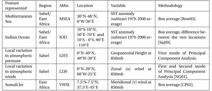
following established conventions for index construction. Details of the techniques employed to construct additional indices as well as data origin are described further in Table 2.1. A total of 35
climate indices are collected over a period of N=57 years from 1951 to 2007. The rainfall data for both the regions is the Gridded Precipitation Climatology Centre (GPCC) V6, gridded at 0.5×0.5 degree resolution. A box average over the geographical coordinates of the Sahel 10◦N-20◦N, 20◦W-35◦E and
East Africa 13◦N-13◦S, 24◦E-55◦E was constructed to build the rainfall data across the regions. The rainfall season in the Sahel has been observed during the months of Jul-Aug-Sep (JAS) and during
the months of Oct-Nov-Dec (OND) in East Africa. For the Sahel region, the monthly values of 34
climate indices are taken from Jan-Jun in a given year and for East Africa region, the monthly values of 33 climate indices are taken from Jan-Sep. We consider two principal components of the LLW
climate index for the Sahel region based on our domain knowledge. The resulting datasets have
dimensions 57Ã ˚U(210+3) and 57Ã ˚U(297+3) for the Sahel and East Africa regions respectively, where the additional 3 variables represent rainfall variables for the three months of the rainfall
season.
Biology:For our first data set, we used publicly available data4containing 71 observations of 101 variables measuring the logarithm of the expression level of 100 genes and the riboflavin production
rate (RPR) in the bacteriumB. subtilis[Büh14]. Our second and third data sets were collected from the Alzheimer’s Disease Neuroimaging Initiative (ADNI). The data sets contained microarray gene expression data collected from 266 male patients and 219 female patients. The cognitive score of
the subjects in each gender was used as the response variable, i.e., CS_M for male patients and CS_F
for female patients.
2http://www.esrl.noaa.gov/psd/data/gridded/data.UDel_AirT_Precip.html 3http://www.esrl.noaa.gov/psd/data/climateindices/list
4http://www.annualreviews.org/doi/suppl/10.1146/annurev-statistics-022513-115545/suppl_
Table 2.1Climate Indices constructed from Reanalysis data to include local variability.
Feature
represented Region Abbr. Location Variable Methodology
Mediterranean Sea Sahel/ East Africa MSEA 30
◦N-46◦N,
6◦W-36◦E
SST anomaly
(subtract 1979-2000 av-erage)
Box average[Row03].
Indian Ocean
Sahel/ East Africa
IOD
10◦S-10◦N,
50◦E-70◦E and
10◦S - 0◦S, 90◦E
- 110◦E
SST anomaly
(subtract 1979-2000 av-erage)
Box average, difference be-tween the two locations
[Saj99].
Local variation in atmospheric pressure
Sahel GHT 0
◦N-40◦N,
40◦W-30◦E
Geopotential Height at 850mb
First mode of Principal Component Analysis.
Local variation in atmospheric winds
Sahel LLW 0◦N-20◦N, 60◦W-25◦E
Zonal (u) wind at 850mb
First and Second mode of Principal Component Analysis[NG01].
Somali Jet East
Africa VWSI
7.5◦S-7.5◦N,
37.5◦E-45◦E
Meridional (v) wind at
850mb Box average[CP02].
2.4.2 Data Preprocessing
The following pre-processing steps were performed after dividing the data into training and test
sets using leave-one-out cross-validation (LOOCV),
1. De-trending: Given the temporal nature of the climate data sets, the predictors and the response variable were detrended to remove seasonal trends. This step was performed only on climate data sets.
2. Normalization: The predictors and the response variable were standardized using their z-scores. Note that the z-scores were computed using the average and the standard deviation
from the training sets.
Due to the indefinite amount of time taken by the PC-stable algorithm for constructing causal
graphs from the microarray gene expression data, we used the training set to select top-100 genes correlated with the response as predictors.
2.4.3 Temporal Constraints
While constructing causal graphs from climate data sets, we explicitly specify certain constraints to obtain temporally coherent causal relationships. Since each predictor contains the monthly
value of a climate index, a causal relationship between monthly values of the same climate index
AM M_1→ AM M_2 where AM M_1 is the value of the climate index in the month of January andAM M_2 is the value in the month of February. On the other hand, we can observe causal relationships between two different climate indices in the same month. For example the climate
indexAM O can effectAM M in the same month or in different months.
2.4.4 Performance Comparison
0 10 20 30 40 50 Methods ASR Accurac y (%)
CFS PC SC
HIT
ON IG
LassoStepRMMHC oneR
(a)African Sahel
0 10 20 30 40 50 Methods EAR Accurac y (%)
CFS PC SC
oneRStepR LassoHITONMMHC
IG
(b)East Africa
0 20 40 60 80 Methods RPR Accurac y (%)
LassoCFSStepR oneRHIT
ON MMHC
SC PC IG
(c)Riboflavin Production Rate
0 10 30 50 70 Methods DX_M Accurac y (%) LassoCFS IG PC oneR MMHC SC StepR HIT ON
(d)Cognitive Score in Male
0 10 30 50 70 Methods DX_F Accurac y (%)
MMHCHITON CFS PConeR
IG SC StepR Lasso
(e)Cognitive Score in Female
0 20 40 60 80 100 Data sets
Reduction in Features (%)
ASR EAR RPR DX_M DX_F
(f )Percentage Feature Reduction
Figure 2.4Mean classification accuracy over leave-one-out cross validation (Accuracy) for the African Sahel
(2.4a), East Africa (2.4b),B. subtilis(2.4c), diagnostic information for Male (2.4d) and Female (2.4e) obtained