ABSTRACT
LIAO, MANG. Optimization Algorithms for Cyber-Physical Security of Wide-Area Power Systems. (Under the direction of Aranya Chakrabortty).
This dissertation work focuses on optimization algorithms for cyber-physical security in wide-area large power system network. In Chapter 2 of this report we first retrospect the power system oscillation model. Our goal is using the measurements from Phasor Measurement Units (PMUs), such as the voltage and current magnitudes and phasors, to estimate the oscillation modes: damping and frequency. To avoid the prior known disturbance input information, we consider the existing well-known modal estimation algorithm, Prony analysis method. The real-time centralized problem is formulated as a global consensus problem, and solved using Alternating Direction Method of Multipliers (ADMM). The power system is divided into multiple non-overlapping areas, each equipped with a local estimator. These local estimators use local sensor measurements of the data from PMUs to carry out a local regression algorithm for generating a local estimate of the characteristic polynomial of the system, and, thereafter, communicate this estimate to a central supervisor. The supervisor computes the average or consensus of all estimates, and broadcasts this consensus variable back to each local estimator to be used in the next round of regression. If all estimates are accurate, then ADMM is guaranteed to converge asymptotically to the true optimal solution of the characteristic polynomial, following which the central supervisor can solve for its roots to obtain the desired eigenvalues. Furthermore, we consider the case of noisy measurements. In the case using the standard ADMM algorithm the estimates cannot be obtained correctly. We fomulate the optimal problem to minimize the influence of the noise into the performance. An efficient approach combining the total least squal (TLS) method and ADMM is provided for the estimation with noisy measurements.
variable will be inaccurate using the standared ADMM in Chapter 2, which, in turn, will contaminate the accuracy of every local estimate. Even a small amount of bias at a single iteration can destabilize the entire estimation process. To combat this, in Chapter 3 we first develop an algorithm to show how ADMM can be used by the central supervisor to catch the identities of malicious estimators by simply tracking the quality of every incoming estimate. This algorithm, however, can become computationally expensive if the network size is large. Therefore, we propose another algorithm where the central supervisor, instead of computing the average, employs a Round-Robin technique to generate the consensus variable, and show that by tracking the evolution of only this consensus variable it is possible to identify the malicious estimators. Both large and covert attacks are considered. Results are illustrated using simulations of a IEEE 68-bus power system model.
If the measurements are noisy it is difficult to detect the identities of the attacked estimator(s) because the injected false bias may remain hidden in the noise. In Chapter 4, we consider to identify the data manipulators in power system estimation loops with noisy measurement. To combat the phenomenon of false bias hidden in the noise, the central supervisor still uses Round-Robin technique with an appropriate order to generate the consensus variable. We show that by tracking the evolution of this consensus variable it is possible to identify which estimators are malicious. We also show that by choosing the correct order based on the TLS estimates it is possible to amplify the attack signatures, thereby reducing false alarms. Numerical results using PMU measurements from IEEE 68-bus power system model illustrate the effectiveness and efficiency of the proposed approaches
© Copyright 2018 by Mang Liao
Optimization Algorithms for Cyber-Physical Security of Wide-Area Power Systems
by Mang Liao
A dissertation submitted to the Graduate Faculty of North Carolina State University
in partial fulfillment of the requirements for the Degree of
Doctor of Philosophy
Electrical Engineering
Raleigh, North Carolina 2018
APPROVED BY:
Alexandra Duel-Hallen Ning Lu
Fen Wu Aranya Chakrabortty
DEDICATION
BIOGRAPHY
ACKNOWLEDGEMENTS
First and foremost, I would like to thank Dr. Aranya Chakrabortty for imparting his knowledge of power system, control theory, and optimization skills on me as well as allowing me venture off into unfamiliar territory and multiple research projects. I cannot thank him enough for his trust and willingness to let me work on the majority of my Ph. D in different state. He has helped me to improve my research skills through involving into several research projects and publishing our own research contributions. Thank you.
To my committee members, Drs. Alexandra Duel-Hallen, Ning Lu, and Fen Wu, your advice, encouragement, and support have been an immense help over the years. I would also like to thank Dr. Di Shi from GEIRI North America Institute, San Jose, CA for mentoring me, sharing your wealth of knowledge of power system with me. Working in GEIRI is my invaluable experience.
I would not have succeeded without the love and moral support from my parents. My parents, you will never know how much I appreciate all the times you were there for me when I felt run down and being right beside me to celebrate the joyous moments. I appreciate your constant love and support throughout my long educational endeavors. To the rest of my family, thank you for various words of wisdom over the years, helpfulness, delicious meals, and wonderful times when we are able to get together and chat up.
TABLE OF CONTENTS
LIST OF TABLES . . . vii
LIST OF FIGURES . . . viii
Chapter 1 Introduction . . . 1
1.1 Contributions . . . 8
1.2 Future Tasks . . . 8
Chapter 2 Wide-Area Oscillation Estimation for Power System using Optimization Algo-rithms . . . 9
2.1 Power System Oscillation Model . . . 10
2.2 Distributed Prony Algorithm with ADMM . . . 13
2.2.1 Prony Algorithm . . . 13
2.2.2 Real-Time Distributed Prony Algorithm using ADMM . . . 15
2.2.3 Noisy Measurements Case . . . 18
2.3 Conclusion . . . 22
Chapter 3 Identifying Data-Manipulators in Power System Estimation Loops . . . 24
3.1 Problem Formulation for Attack Identification . . . 25
3.2 Data Manipulations with General Biases . . . 28
3.2.1 Detection of attacks . . . 28
3.2.2 S-ADMM for Identifying Malicious PDCs . . . 29
3.2.3 Round-Robbin ADMM for Detecting the Malicious Users . . . 32
3.2.4 Random Order of RR-ADMM . . . 36
3.3 Data Manipulations with Small Biases . . . 38
3.3.1 S-ADMM for Detecting Malicious Users with Small Biases . . . 38
3.3.2 RR-ADMM for Detecting Malicious Users with Small Biases . . . 41
3.4 Comparison between S-ADMM and RR-ADMM . . . 44
3.5 Simulation Results . . . 46
3.6 Conclusion . . . 55
Chapter 4 Identifying Data-Manipulators with Noisy Measurements . . . 57
4.1 Problem Formulation for Attack Identification . . . 57
4.2 Proposed Round-Robbin ADMM . . . 58
4.2.1 RR-ADMM with Local TLS Estimates . . . 60
4.3 Simulation results . . . 64
4.4 Conclusions . . . 66
Chapter 5 Identifying Data Manipulators in Distributed Wide-Area Control Loops of Power Systems . . . 68
5.1 Problem Formulation for Attack Identification . . . 69
5.1.2 Data updated by the individual PDCs . . . 72
5.1.3 When the VMs at one or multiple areas are faulted or attacked . . . 72
5.2 Identify the faulted or attacked VMs . . . 74
5.3 Identify the attacked VMs covertly . . . 76
5.3.1 RR controller in fault-free case . . . 77
5.3.2 RR Sparse controller in fault case . . . 80
5.4 Simulation . . . 85
5.5 Conclusion . . . 90
Chapter 6 Concluding Remarks and Future Research . . . 91
6.1 Conclusion . . . 91
6.2 Future Research Directions . . . 92
References . . . 94
Appendix . . . 105
Appendix A Flow Charts . . . 106
LIST OF TABLES
LIST OF FIGURES
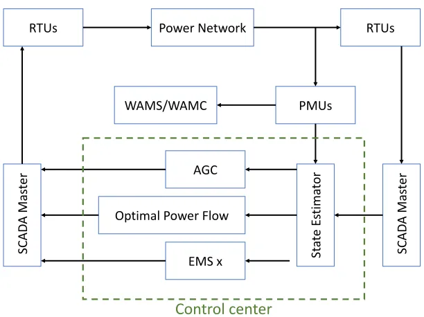
Figure 1.1 A schematic block diagram of a power network, a SCADA system, and a control
center. . . 3
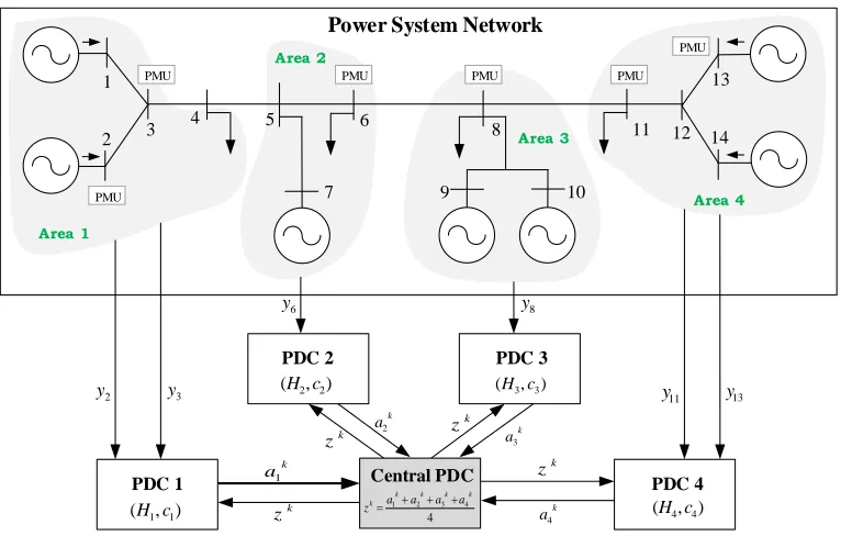
Figure 2.1 Distributed architecture for a 4-area power system network. . . 16
Figure 2.2 The trajectories of the data from each local PDC using S-ADMM. . . 18
Figure 2.3 The trajectories of the data from each local PDC using S-ADMM. . . 19
Figure 2.4 Values of the real parts of the four estimated inter-area modes using S-ADMM and TLS-ADMM with noisy measurements, respectively. True values ofσi are shown by dashed lines. . . 22
Figure 3.1 The trajectories of the data from each local PDC using S-ADMM with biases. . . 27
Figure 3.2 The timing diagram of the communication between the central and local PDCs. . . 29
Figure 3.3 Evolution of the norms of the local estimates, and the averagezzzkbefore and after detection using S-ADMM. For convenience, we only show the first element ofzzzk. . 33
Figure 3.4 Evolution of the averagezzzkbefore and after detection using RR-ADMM. For conve-nience, we only show the first element ofzzzk. . . 37
Figure 3.5 Evolution of the norms of the local estimates, and the averagezzzkavbefore and after detection of attack with small biases using S-ADMM. For convenience, we only show the first element ofzzzkav. . . 40
Figure 3.6 The response of zzzk before and after detection of attack with small biases using RR-ADMM . . . 44
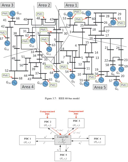
Figure 3.7 IEEE 68-bus model . . . 47
Figure 3.8 Architecture for a 5-area power system network with 2 malicious PDCs. . . 47
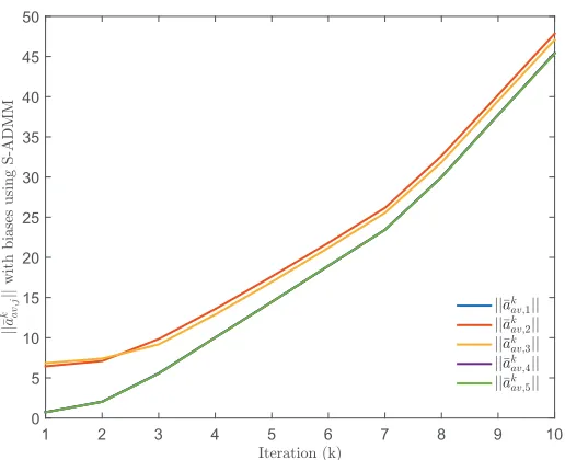
Figure 3.9 Evolution of||aaa¯kav,j||when S-ADMM is run under attacks. . . 48
Figure 3.10 Values of the real parts of the four inter-area modes before and after detection using S-ADMM. True values ofσiare shown by dashed lines. . . 49
Figure 3.11 Evolutions of||zzzkav||and the first four elements ofzzzkav when S-ADMM is run under attacks. . . 49
Figure 3.12 Evolutions of||zzzk||when RR-ADMM and S-ADMM are run under attacks. . . 50
Figure 3.13 Values of the real parts of the four inter-area modes before and after detection with RR-ADMM. True values ofσiare shown by dashed lines. . . 51
Figure 3.14 ||zzzkrr||with random order of RR-ADMM. . . 51
Figure 3.15 The response of||¯aaakav,j||with sparse biases and non-sparse biases using S-ADMM. 52 Figure 3.16 The response of||zzzkrr||with sparse biases and non-sparse biases using RR-ADMM. 53 Figure 3.17 The response of||zzzkav||with sparse biases and non-sparse biases using S-ADMM. . 53
Figure 3.18 Evolutions of||aaa¯kav,j||with multiple biases and different values ofρ using S-ADMM. 54 Figure 3.19 Values of the real parts of the four estimated inter-area modes before and after detection using S-ADMM with small biases. True values ofσiare shown by dashed lines. . . 55
Figure 4.3 Evolutions of average values ofzzzwhen TLS-ADMM and RR-ADMM are run under attacks. . . 65 Figure 4.4 Values of the real parts of the four inter-area modes before and after detection with
Chapter 1
Introduction
Reliable electricity supply via the modern power grid is fundamentally supported by the underlying cyber systems. Power system security involves two main aspects: physical security and cyber security. Physical security represents the ability of a power system to maintain a normal working state in the presence of severe disturbances. Cyber security refers to the security of the communication networks and computer systems which support the power system operation. Weaknesses in cyber security can threaten the physical security of the power systems due to the strong correlation of the physical and cyber systems [1–6].
In the same year, major blackouts also happened in Europe, such as Denmark, Sweden, and Italy [9]. In 2008, the public transport system in Poland was hacked remotely, while in 2010 the Stuxnet worm attacked Iran’s Natanz nuclear fuel-enrichment facility. On 23 December 2015, a synchronized and coordinated cyber-attack compromised three Ukrainian regional electric power distribution companies, resulting in power outages affecting approximately 225000 customers for several hours [10]. With several thousands of networked PMUs being scheduled to be installed in the United States by 2020, exchange of Synchrophasor data between balancing authorities for any type of wide-area control will involve several thousands of Terabytes of data flow in real-time per event, thereby opening up a wide spectrum of opportunities for adversaries to induce data manipulation attacks [11–13], denial-of-service attacks [14], GPS spoofing [15], attacks on transmission assets [16], and so on. The challenge is even more aggravated by the gradual transition of WAMS from centralized to distributed in order to facilitate the speed of data processing [19–21]. Unlocking the tremendous potential of the smart grid strongly depends on the security of this system. From the advent of the smart grid concept, security has always been a primary concern. In the 2009 White House Cyberspace Policy Review, the US federal government was asked to ensure that security standards are developed and adopted to avoid creating unexpected opportunists to penetrate these systems or conduct large-scale attacks [17]. The US National Institute of Standards and Technology (NIST) has provided guidelines for developers and policy makers, covering cyber security requirements of the smart grid that should be included from the beginning of the development process [18].
RTUs Power Network RTUs
WAMS/WAMC PMUs
St
at
e
Es
tim
at
or
AGC
Optimal Power Flow
EMS x SC
AD
A
M
as
te
r
SC
AD
A
M
as
te
r
Control center
Figure 1.1: A schematic block diagram of a power network, a SCADA system, and a control center.
operator in the control center with hopefully accurate information at all times. The state estimation results reflect the real time power grid operation state and are essential for operators to make decisions in order to maintain security and stability of the system. Many power system applications, such as economic dispatch (ED), contingency analysis, and so forth, rely on the results of state estimation [25, 39]. Attack can degrade the performance of the state estimates [26], and even worse destroy the security and stability of the system [27] and have catastrophic consequences [28]. Therefore, detecting the identities of the data manipulators has become a significant and inevitable problem in power systems.
estimation-based mitigation strategies to secure the grid against many of these attacks [33–36]. In general, research on FDIAs mainly focuses on the following three aspects: theoretical research, application research, and defensive research [37]. In theoretical research, the challenge is the construction of injected vectors capable of evading detection by the control center under different situations [38], for example, when the attacker has limited access to meters, incomplete information, false topology, or an AC power flow model is used; the attacker then injects bad data into meters. In application research, the purpose is to analyze the impacts of FDIAs on power system operation, mainly on EMS and market management systems (MMS), such as economic dispatch and congestion managements. In defensive research, the aim is proposing defense strategies from the viewpoint of the system operator. In [37] Liang et al. summarized the existing works that can be categorized as shown in Table 1.1. The fundamental approach behind many of these designs is based on the so-called idea of Byzantine consensus [72–74], a fairly popular topic in distributed computing, where the goal is to drive an optimization or optimal control problem to a near-optimal solution despite the presence of a malicious agent. In practice, however, this approach is not acceptable to most WAMS operators as they are far more interested in finding out theidentityof a malicious agent if it exists in the system, disconnect it from the estimation or control loop, and continue operation using the remaining non-malicious agents rather than settling for a solution that keeps the attacker unidentified in the loop. This basic question of how tocatchmalicious agents in distributed wide-area monitoring applications is still an open challenge in the WAMS literature.
Table 1.1: Overview of FDIA researches
FDIA research Categories References
Construct a valid FDIA under certain constraints
[12, 28, 39–42]
Theoretical researches on con-strcting a valid FDIA
Construct a valid FDIA with incom-plete information of matrix
[43–46]
Construct a valid FDIA with topol-ogy being falsified
[47–49]
Construct a valid FDIA under AC power flow model
[50–52]
Economic attack [48, 49, 53–55] Application researches on the
im-pacts of FDIAs
Load redistribution attack
[56, 57] Energy deceiving
attack
[58] Protect a set of ba-sic measurements
[12, 39, 59, 60] Defense strategies against FDIAs PMU-based
protec-tion
[61–64] Other ways of
defending against FDIAs
[65–71]
manipulators. We consider the identification in these cases of both general false-data injection and covert bias. Also the detection of malicious users with noisy measurements is analyzed.
Thus, at any iteration, the local estimators receive PMU measurements from within their own respective areas, run a local consensus algorithm, and communicate their estimates to a central estimator. The central estimator averages all estimates, and broadcasts the average back to each local estimator as the consensus variable for their next iteration. It was shown that this average value converges to the global solution as the number of iterations tends to infinity. Besides, we consider the case of noisy measurements. Then the optimization problem is changed to minimize the influence of the noise into the performance. In this case, using the standard ADMM algorithm the oscillation modes cannot be estimated correctly. Thus we develop the traditional ADMM and combine it into total least squal (TLS) method, and then the correct estimates are obtained with noisy measurements.
However, due to the high cost associated with dedicated fiber-optic communication networks, the communication between the local PDCs and the central PDC is most likely to happen over an open wide-area communication network. These networks are quite vulnerable to hacking. The key question, therefore, is how to catch malicious agents in distributed wide-area monitoring applications. In Chapter 3, we address this question in the context of identifying malicious data-manipulators in distributed optimization loops for wide-area oscillation monitoring. The specific application of our interest is the estimation of electromechanical oscillation modes or eigenvalues from streaming PMU data following a small-signal disturbance in the grid [75, 76]. If one or more of the local estimates are manipulated by attackers, then the resulting consensus variable will be inaccurate using ADMM mentioned in Chapter 2, which, in turn, will contaminate the accuracy of every local estimate. Even a small amount of bias at a single iteration can destabilize the entire estimation process. To combat this, we first develop an algorithm to show how ADMM can be used by the central supervisor to catch the identities of malicious estimators by simply tracking the quality of every incoming estimate. This algorithm, however, can become computationally expensive if the network size is large. Therefore, we propose another algorithm where the central supervisor, instead of computing the average, employs a Round-Robin technique to generate the consensus variable, and show that by tracking the evolution of only this consensus variable it is possible to identify the malicious estimators. Both large and covert attacks are considered.
based regression no longer yields accurate results as least square (LS) is inherently a biased estimator. Instead a more robust and noise-tolerant version of LS, namely, total least squares (TLS) [81], need to be used in such scenarios. We, therefore, first develop a distributed version of TLS using ADMM. In Chapter 4 thereafter we show that if some of the local estimators are compromised then attackers at these estimators may send corrupted values of their TLS estimates, and destabilize the estimation loop completely within a few iterations. Since the measurements are noisy it is difficult to detect the identities of the attacked estimator(s) since the injected false bias may remain hidden in the noise. To combat this, in Chapter 4 we propose an algorithm where the central supervisor, instead of computing the average as in the usual ADMM, employs a deterministic ordered Round- Robin technique to generate the consensus variable. We show that by tracking the evolution of this consensus variable it is possible to identify which estimators are malicious. We also show that by choosing the correct order based on the TLS estimates it is possible to amplify the attack signatures, thereby reducing false alarms.
simply tracking the magnitude of every control input covertly. In the normal case, the system uses LQR controller for minimizing the cost. When the attacker accesses the network, the firewall [96] or intrusion detection system (IDS) [97] can detect the intruder and broadcast the alarm. The system changes to the sparse controller with RR technique. At this time the attacker just accesses the network, not intrudes the VMs. Each VM keeps the same calculation of the inputs after the alarm. So the attacker believes that the system always uses the RR sparse controller to calculate the inputs and cannot perceive the detection period. We illustrate effectiveness of the attack localization algorithms using simulation results on an IEEE 68-bus power system model.
1.1
Contributions
1. Devolop Standard ADMM and Round Robin ADMM for detecting the identities of the data manipulators with general biases in wide-area power system estimation loops.
2. Devolop Standard ADMM and Round Robin ADMM for detecting the identities of the data manipulators with covert biases in wide-area power system estimation loops.
3. Devolop the algorithm which is combined TLS and Round Robin ADMM for detecting the identities of the data manipulators with noisy measurements in wide-area power system estimation loops.
4. Design the sparse controller based on Round-Robin technique for identifying the attacked or faulted virtual machines in wide-area power system control loops.
1.2
Future Tasks
1. Identify the data manipulators with other attack methods, such as denial-of-service attack and replay attack.
Chapter 2
Wide-Area Oscillation Estimation for
Power System using Optimization
Algorithms
of the characteristic polynomial of the system, and, thereafter, communicate this estimate to a central supervisor. The supervisor computes the average or consensus of all estimates, and broadcasts this consensus variable back to each local estimator to be used in the next round of regression. If all estimates are accurate, then ADMM is guaranteed to converge asymptotically to the true optimal solution of the characteristic polynomial, following which the central supervisor can solve for its roots to obtain the desired eigenvalues. Furthermore, we consider the case of noisy measurements. When measurements are corrupted by noise, the standard least-squares based regression no longer yields accurate results as LS is inherently a biased estimator. Instead a more robust and noise-tolerant version of LS, namely, Total Least Squares (TLS) [81], need to be used in such scenarios. For reducing the effect of noise on the estimates, a novel algorithm, called TLS-ADMM is proposed. The actual implementation of this algorithm can be easily adapted to the cyber-physical architecture [82]. Simulation results on a IEEE 68-bus power system model illustrates its effectiveness.
2.1
Power System Oscillation Model
Consider a power system network consisting ofnsynchronous generators andnl loads connected by a given topology. Without loss of generality, we assume buses 1 throughnto be the generator buses and busesn+1 throughn+nlto be the load buses. LetPiandQidenote the total active and reactive powers injected to theithbus (i=1, . . . ,m+nl) from the network that is calculated as:
Pi= n+nl
∑
k=1
Vi2rik/z2ik+ViVksin(θik−αik)/zik, (2.1a)
Qi= n+nl
∑
k=1
Vi2xik/z2ik−ViVkcos(θik−αik)/zik, (2.1b)
whereVi∠θi is the voltage phasor at theith bus.rik and xik in (2.1) are the resistance and reactance of the transmission line joining busesiandk, respectively.θik=θi−θk,zik=
q
r2ik+x2ik, andαik=
differential-algebraic equations (DAE) [83] as follows:
˙
δi=ωs(ωi−1) (2.2a)
Miω˙i=Pmi−Pei−Di(ωi−1),i=1, ..,m, (2.2b)
with associated power balance equations given by
Pei+Pi−PLi =0,i=1, . . . ,n, Qei+Qi−QLi =0,
Pk−PLk=0,k=n+1, . . . ,n+nl,
Qk−QLk =0, (2.3)
whereδi, ωi,Mi,Di,Pmi,Pei, and Qei denote the internal angle, speed, inertia, damping, mechanical
power, active and reactive electrical powers produced by the ith generator, respectively.PLk andQLk
denote the active and reactive powers of the loads at thekthbus. The DAE in (2.2) can be converted to a system of purely differential equations by relating the algebraic variablesVi andθiin (2.1) to the system state variables(δ,ω)and then substituting them back in (2.2) via Kron reduction. The resulting system
is a fully connected network ofmsecond-order oscillators withl≤n(n−1)/2 tie-lines. Let ˜Ei=Ei∠δi denote the internal voltage phasor of theithmachine. Fori=1, . . . ,mthe electromechanical dynamics of theithgenerator inKron’s form can be written as:
˙
δi=ωs(ωi−1), (2.4a)
Miω˙i=Pmi−Pi−Di(ωi−1), (2.4b)
Pi=
∑
kEiEk
Xik
Zik2 sin(δik)− Rik
Zik2 cos(δik)
, (2.4c)
(δi0,1)results in the small signal state space model: ∆δ˙ ∆ω˙ =
0m×m ωsIm×m M−1L M−1D
| {z }
A ∆δ ∆ω + 0 M−1eee
j
| {z } B
u,
yyy=col(∆δi,∆ωi), for i∈S, (2.5)
where∆δ =
∆δ1 · · · ∆δm T
,∆ω =
∆ω1 · · · ∆ωm T
,Im×mdenote them×midentity matrix.M = diag(Mi)andD=diag(Di)are them×mdiagonal matrices of the generator inertias and damping factors, respectively.eeejis the jthunit vector with all elements zero but the jthelement that is 1, considering that the input is modeled as a change in the mechanical power in the jthmachine. Since we are interested only in the oscillatory modes or eigenvalues ofA, this assumption is not necessary. The input can be modeled in any other feasible way, such as faults and excitation inputs. The matrixL in (2.5) is the
m×mLaplacian matrix of the form:
[L]i,j=
EiEj
Z2
i j
Xi jcos(δi0−δj0) +Ri jsin(δi0−δj0)
i6= j,
[L]i,i=− n
∑
k=1
[L]i,k. (2.6)
Let ˆλidenote theitheigenvalue of the matrixM−1L. The largest eigenvalue of this matrix is equal to 0, and all other eigenvalues are negative, i.e. ˆλm≤ · · · ≤λˆ2<λˆ1=0. The eigenvalues ofA are given
byλi= (−σi±jΩi),(j= √
−1), whereΩi= q
|λˆi|denotes theithosscillation frequency, andσi>0 denotes theithdamping factor.
Our purpose is to estimate the oscillation modes, frequencyΩand damping factorσ from the PMU
2.2
Distributed Prony Algorithm with ADMM
For estimating the oscillation modes based on PMU measurements, we introduce the existing well-known modal estimation algorithm, Prony analysis method, and its real-time distributed architecture in this section.
2.2.1 Prony Algorithm
Consider a set ofNPMU measurementsyyy(t) =col(y1(t)· · ·yN(t))are available att=0,1, . . . ,M, in a given power system network described in Section II. Following the linearized state space model shown in Equation (2.5), one can write the continuous-time transfer function between the inputu(t)and output
yp(t)as below [84]:
Gp(s) =Yp(s)
U(s) = n
∑
i=1 rp,i
s−λi
, (2.7)
whereλiis theithpair of eigenvalues, corresponding to theithpair of oscillatory modes of the system,
rp,iis the residue or amplitude ofithmode, andnis the total system order. If we apply an impulse as input to the system, the outputyp(t)can be written as
yp(t) = n
∑
i=1
rp,ie(−σi+jΩi)t+r∗p,ie(
−σi−jΩi)t,p=1,· · ·,N. (2.8)
Note that regardless input is an impulse or a step unit, the linearized system response will always be a sum of exponential terms [75, 76]. This is the form that the Prony method can be applied for modal estimation. Whenyp(t)is sampled at a constant sampling period∆t, we have the following discrete form:
yp(k) = n
∑
i=1
rp,izki, (2.9)
wherezi=e(−σi±jΩi)∆t. The modal estimation objective is to find the damping factorsσi, the
yi(t)with a uniform sampling period ofT, a generic expression for thez-transform ofyi(m),yi(t)|t=mT, (m=0,1, . . . ,M), can be written as
yi(z) =b0i+b1iz −1+b
2iz−2+· · ·+b2niz−2n 1+a1z−1+a2z−2+· · ·+a2nz−2n
, (2.10)
wherea’s andb’s are constant coefficients of the characteristic polynomial and the zero polynomial, respectively. The roots of the characteristic polynomial will provide the discrete-time poles of the system. One can, therefore, first estimate the coefficient vector aaa:{a1, . . . ,a2n}, compute the discrete-time poles, and finally convert them to the continuous-time poles to obtainσk andΩk, fork=1, . . . ,2n, as follows [75, 76]:
Step 1.Solve foraaafrom
yi(2n)
yi(2n+1) .. .
yi(2n+`)
| {z } ccci =
yi(2n−1) · · · yi(0)
yi(2n) · · · yi(1) ..
. ...
yi(2n+`−1) · · · yi(`)
| {z }
H H Hi
−a1
−a2
.. . −a2n
| {z } aaa
, (2.11)
where`is an integer satisfying 2n+`≤M−1. ConcatenatingccciandHHHiin (2.11) fori=1, . . . ,p, one can findaaaby solving a LS problem
min a a a 1 2|| H H H1 .. .
HHHp
aaa− ccc1 .. . cccp
||2, (2.12)
where|| · ||denotes the 2-norm of a vector.
Step 3.The final step is to find the residuesrrriin (2.8). This can be done by forming the following so-calledVandermondeequation and solving it forrrr1throughrrrn.
yi(0)
yi(1) .. .
yi(M) =
1 1 · · · 1
(z1)1/T (z2)1/T · · · (zn)1/T ..
. ... ...
(z1)M/T (z2)M/T · · · (zn)M/T
r1
r1∗
.. .
rn
rn∗
. (2.13)
The centralized approach, however, becomes computationally untenable as more and more PMUs are installed in the system. Instead a distributed solution is much more preferable. In the next subsection, the LS problem (2.12) is reformulated as a global consensus problem over a distributed network and ADMM is utilized for findingaaa.
2.2.2 Real-Time Distributed Prony Algorithm using ADMM
1
2
13
14
4 5 6
8
7 9 10
11 12
3
PDC 1
PDC 2 PDC 3
PDC 4 )
, (H1c1
PMU
PMU
PMU PMU PMU
PMU Area 1 Area 2 Area 3 Area 4 ) ,
(H2c2 (H3 ,c3)
) , (H4c4 3
y 2 y
6
y y8
11 y y13
Central PDC 4 4 3 2 1 k k k k
k a a a a
z k
a1
k
a2 k
a3
k a4 Power System Network
k z k z k z k z
Figure 2.1: Distributed architecture for a 4-area power system network.
rewritten as
min a aa1,...,aaaN,zzz
N
∑
i=1
1
2||HHHˆiaaai−cccˆi||
2,
sub ject to aaai−zzz=0, (2.14)
for i=1, . . . ,N, whereaaai is the vector of the primal variables, zzz is the global consensus variable, ˆ
H
HHi= [HHHTi1,HHH T
i2, . . . ,HHH T
imi]T, and ˆccci= [ccci1,ccci2, . . . ,cccimi]
T. Each block element of ˆHHH
iand ˆcccican be constructed after the disturbance using the data matrices shown in (2.11). The estimators can wait up to a certain number of samples, say 2n+`as indicated in (2.11), and gather the local measurements up to that iteration.
Theaugmented Lagrangianfor (2.14) is defined as
Lρ=
N
∑
i=1
(1
2HHHˆiaaai−cccˆi
2
+wwwTi (aaai−zzz) +
ρ
2aaai−zzz
2),
wherewwwiis the vector of thedual variables, or the Lagrange multipliers associated with (2.14), andρ>0 denotes thepenalty factor. Then the optimal problem in (2.14) can be solved in a distributed way using ADMM [80], which reduces to the following set of recursive updates:
w w
wki =wwwk−i 1+ρ(aaaki−zzzk), (2.15a)
a a
aki+1= ((HHHˆi)THHHˆi+ρIII)−1((HHHˆi)Tcccˆi−wwwki +ρzzz k
), (2.15b)
zzzk+1= 1
N
N
∑
i=1 a
aaki+1. (2.15c)
To distinguish it from other variants of ADMM to be proposed later in the paper, we will refer to (2.15) as the standard ADMM, or S-ADMM in short. In [19] we developed the cyber-physical architecture by which local PDCs and the central PDC can exchange information between each other for executing S-ADMM. We summarize that architecture as follows. Consider thekthiteration.Step 1)any local PDC
iruns the dual-primal update for (wwwki,aaaki+1) using (2.15a) and (2.15b), after receiving the consensus variablezzzkfrom the central PDC;Step 2)the local PDCitransmitsaaaki+1to a central PDC;Step 3)the central PDC calculates the consensus variablezzzk+1using (2.15c);Step 4)the central PDC broadcasts
zzzk+1to the local PDCs in each area for their next update. Since the LS problem is convex, therefore ask→∞,zzzk in (2.15c) converges tozzz∗ which is the solution of the centralized problem (2.14). Also, because of consensus, everyaaakjconverges tozzz∗, 1≤ j≤N;Step 5)finally, the central PDC estimates the eigenvalues of the small-signal model by solving for the roots of the characteristic polynomial given by
zzz∗.
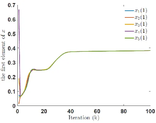
Figure 2.2: The trajectories of the data from each local PDC using S-ADMM.
dynamics simulation routines simuand the data filedata16m.m[85]. We setρ=10−6. The synchronous
generators are assumed to have 6th-order models for simplicity. Since there are 16 generators, our proposed algorithm should ideally solve a 96th-order polynomial. However, our previous work on this model as reported in [19] show that choosing 2n=40 yields a reasonably satisfactory estimate of the inter-area modes. From the Fig. 2.2, the data from each PDC will be convergent to the same value using S-ADMM. Then we can use the equilibrium value of the data from each local PDC to calculate the oscillation modes. Fig. 2.3 shows four selected estimated modesσ per iteration. They converge to their
global values within 25 iterations. The dashed lines show the actual values ofσ for these four modes
obtained from PST.
2.2.3 Noisy Measurements Case
The ordinary LS estimator (2.12) is biased when the measurement vectoryyy(t)is noisy. Let ˜yi(j) =yi(j) +
εi(j)be the noisy measurement, whereεi(j)denotes the noise or any other measurement imperfection
0 5 10 15
Iteration
(k)
20 25 30
E
stimates
of
<
i 0.3 0.35 0.4 0.45 0.5<
1<
2<
3<
4Figure 2.3: The trajectories of the data from each local PDC using S-ADMM.
rewritten as
˜
HHHi=
yi(2n−1) +εi(2n−1) . . . yi(0) +εi(0)
yi(2n) +εi(2n) . . . yi(1) +εi(1) ..
. ... ...
yi(2n+`−1) +εi(2n+`−1) . . . yi(`) +εi(`)
=HHHi+εHi; (2.16)
˜
ccci= ˜
yi(2n)
˜
yi(2n+1) .. .
˜
yi(2n+`) =
yi(2n) +εi(2n)
yi(2n+1) +εi(2n+1)
.. .
yi(2n+`) +εi(2n+`)
Now our goal is change to reduce the effect of noise on the estimates. Then the optimization problem (2.14) can be reformulated as:
min a
N
∑
i=1
1 2||εi||
2,
sub ject to (HHH˜i−PPPHεi)aaai=ccc˜i−PPPClεiPPPCr, a
aai=zzz, (2.18)
wherePPPH= [III`+1,0001×(`+1)],III`+1is a(`+1)×(`+1)identity matrix,PPPCl = [0001×(`+1),III`+1], andPPPCr=
[1,0001×(2n−1)]T. The optimization problem (2.18) is commonly referred to as Total Least Squares or
TLS [81]. To solve (2.18) in a distributed way, we follow the general ADMM approach, and define the
augmented Lagrangianfor (2.18) as
Lρ= N
∑
j=1
1 2||εi||
2+wwwT
i(aaai−zzz) +
ρ1
2||aaai−zzz||
2+uuuT
i
(HHHi−PPPHεi)aaai−ccci+PPPClεiPPPCr
+ρ
2||HHHi−PPPHεi)aaai−ccci+PPPClεiPPPCr||
,
corresponding update equations, similar to (2.15), can be written as:
εik+1=
III+ρ(PPPCl−PPPH) T(PPP
Cl−PPPH)
−1
×
P
PPTHuuuki(aaaki)T−PPPCT luuu
k
iPPPTCr−ρ(PPPCl−PPPH) T(HHH
iaaaki−ccci)(PPPCr−aaa
k i)T
×
III+ (PPPCr−aaa
k
i)(PPPCr−aaa
k i)T
−1
, (2.19a)
a a aki+1=
ρ1III+ρ(HHHi−PPPHεik+1)T(HHHi−PPPHεik+1) −1
×
ρ1zzzk−wwwki −(HHHi−PPPHεk+1)Tuuuki +ρ(HHHi−PPPHεik+1)T(ccci−PPPClε
k+1
i PPPCr)
, (2.19b)
u u
uki+1=uuuki +ρ
(HHHi−PPPHεik+1)aaaki+1−ccci+PPPClε
k+1
I PPPCr
, (2.19c)
zzzk+1= 1
N
N
∑
j=1 a
aakj+1, (2.19d)
w
wwki+1=wwwki+ρ1(aaaki+1−zzz
k+1). (2.19e)
We refer to (2.19) as TLS-ADMM. The actual implementation of this algorithm can be easily adapted to the cyber-physical architecture that we recently proposed in [82]. We summarize that architecture as follows. Consider thekthiteration.Step 1)any local PDCiruns the primal update for (εik+1andaaaki+1) using (2.19a) and (2.19b), after receiving the consensus variablezzzk from the central PDC;Step 2)the local PDCitransmitsaaaki+1to a central PDC;Step 3)the central PDC calculates the consensus variable
zzzk+1 using (2.19d);Step 4)the central PDC broadcastszzzk+1to the local PDCs in each area for their next update;Step 5)the local PDCiupdates the dual variablesuuuik+1andwwwki+1using (2.19c) and (2.19e). Since the optimal problem in (2.18) is convex, therefore ask→∞,zzzk in (2.19d) converges tozzz∗which is the solution of the optimization problem (2.18) [80]. Also, due to consensus, everyaaaki converges to
zzz∗, 1≤ j≤N;Step 6)finally, the central PDC estimates the eigenvalues of the small-signal model by solving for the roots of the characteristic polynomial given byzzz∗.
0 500 1000 Iteration (k) -0.4
-0.2 0 0.2 0.4 0.6 0.8 1
Estimates
of
<i
using
TLS
-ADMM
<1
<2
<3
<4
0 500 1000
Iteration (k) 0.3
0.35 0.4 0.45 0.5
Estimates
of
<i
using
S
-ADMM
<1
<2
<3
<4
Figure 2.4: Values of the real parts of the four estimated inter-area modes using S-ADMM and TLS-ADMM with noisy measurements, respectively. True values ofσiare shown by dashed lines.
The dash lines shows the true values of the damping coefficients σi for the four dominant inter-area oscillation modes, while the solid lines show their estimated values. In the left figure, the estimates ofσi,
obtained via TLS-ADMM, match their true values. In the right figure, however, the estimates obtained using S-ADMM do not match the true values. Same holds for the imaginary parts of the modes.
2.3
Conclusion
Chapter 3
Identifying Data-Manipulators in Power
System Estimation Loops
local estimate. Even a small amount of bias at a single iteration can destabilize the entire estimation process. To combat this, we first develop an algorithm to show how ADMM can be used by the central supervisor to catch the identities of malicious estimators by simply tracking the quality of every incoming estimate. This algorithm, however, can become computationally expensive if the network size is large. Therefore, we propose another algorithm where the central supervisor, instead of computing the average, employs a Round-Robin technique to generate the consensus variable, and show that by tracking the evolution of only this consensus variable it is possible to identify the malicious estimators. Both large and covert attacks are considered. To combat this, we propose an algorithm where the central supervisor, employs the deterministic ordered Round-Robin technique to generate the consensus variable. We show that by tracking the evolution of this consensus variable it is possible to identify which estimators are malicious. We analyze the convergence properties of the proposed algorithms, and illustrate their effectiveness using simulation results on a IEEE 68-bus power system model.
3.1
Problem Formulation for Attack Identification
ADMM starts, or at anyk>0 while ADMM is in progress.
Because the ISO does not know that the message is corrupted, it will still calculate the consensus variable by averaging the estimates obtained from all individual local PDCs. Thuszzzk in (2.15c) will become
zzzk=∆k+ 1
N
N
∑
i=1 a aaki
!
, (3.1)
where∆k=N1 ∑ j=1,j∈S
∆kj !
. Notice that here we consider any number of local PDCs to be attacked, as long as there is at least one unattacked PDC, and that the bias∆kj may be time-varying and of arbitrary magnitude.
Although the matricesHHHki andcccki are time-varying matrices, i.e., they are functions of the iteration index k, the convexity of the LS problem will yield the same solution zzz∗ if these two matrices are replaced by two constant matricesHHHi andccci, respectively, where the latter is constructed by waiting over a certain number of iterations, and gathering all local measurements up to that iteration. Denoting
Aj:= ((HHHˆ j)THHHˆ j+ρIII2n)−1, andCj:= (HHHˆ j)Tcccj, following the expression of the consensus variable with bias as in (3.1), the S-ADMM algorithm in (2.15) can be written in a state-variable form:
a a ak+1
aaak
= L LL11 LLL12
III 000
| {z } LLL
aaak
a a ak−1
+ P PP 0 00 ∆ k , (3.2)
whereaaak=
aaak1
aaak2
.. .
a aakN
,LLL12=−
ρA1
N . . .
ρA1
N ..
. . .. ...
ρAN
N . . .
ρAN
N
,PPP= ρA1 ρA2 .. .
ρAN
,LLL12=−
ρA1
N . . .
ρA1
N ..
. . .. ...
ρAN
N . . .
ρAN
Figure 3.1: The trajectories of the data from each local PDC using S-ADMM with biases.
L LL11=
I+(2−NN)ρA1 2ρNA1 . . . 2ρNA1 2ρA2
N I+
(2−N)ρ
N A2 . . .
2ρA2
N ..
. ... ... ...
2ρAN
N . . .
2ρAN
N I+
(2−N)ρ
N AN
.
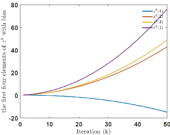
The rows ofLLLin (3.2) add up to 1, and so when∆kj=0 then the trajectories ofaaaki for everyi=1, . . . ,N converge asymptotically to consensus, as shown in [80]. However, when the arbitrary disturbance∆kj is added then these trajectories will diverge unless∆kj is chosen in a special way so that its entries corresponding to the consensus modes are exactly zeros. That, however, is very unlikely to happen as the attacker will not know the matrixLLLprior to the attack, and, therefore, cannot use any information about its consensus properties for designing∆kj. In any case, the attacker would benefit most ifaaaki start diverging, implying that she has been able to destabilize the estimation loop. Fig. 3.1 shows the trajectories of the data from each PDC from the IEEE 68-bus power system model using S-ADMM algorithm as in Chapter 2. The system is divided into 5 areas, each with one local PDC and 3 PMUs. The simulated measurements are obtained using the Power System Toolbox (PST) nonlinear dynamics simulation routines simuand
because of the false-data injections. Thus, we cannot estimate the correct values of the oscillation modes in this case. Detecting the identity of the corrupted PDC, therefore, is crucial to retain normal operation of the loop.
In the following sections, we propose a variety of algorithms to catch the identities of these data manipulators, starting with S-ADMM and then its round-robbin version. We also consider the case when ∆kj is small or covert, and show how S-ADMM can be used for the detection by reducing the penalty parameterρ. In that situation the round-robbin algorithm can also detect the identities of the manipulators by monitoring the dual variable wwwkj without requiring any knowledge of the individual estimatesaaakj, thereby saving computation cost.
It should also be noted that the algorithms presented in the following sections are solely based on the computed values of the primal and dual variables of ADMM. They do not need any information about the power system model parameters, nor the PMU measurementsyi. This is the main difference between our work and the work in [87]. In [87], the authors derived detectability results based on the properties of the state matrixLLLin (3.2). In our problem set-up, however,LLLconsists of the Hankel matrices ˆHHHiand ˆccci, both of which are filled with the measured outputsyi. The inherent assumption is that the central PDC does not have direct access to anyyi, and therefore, does not know anything about the matrixLLL. It only has access to the estimatesaaaiand the dual variableswwwi,i=1, . . . ,N, and, therefore, must algorithmically figure out the detection and identification mechanisms based on these two variables only. This is the main contribution of the paper, compared to the model-based results of [87]. The time line for executing ADMM and the attack localization algorithms is shown in Fig. 3.2.
3.2
Data Manipulations with General Biases
3.2.1 Detection of attacks
t=0 t=t1 t=t2 t=tf 1. Fault occurs in the power system 2. PMUs send data to local PDCs
1. PDCs finish gathering (Hi, ci)
2. ADMM starts 3. Data manipulation starts Pre-fault equilibrium 1. Central PDC localizes the faulty PDC 2. ADMM continues with the non-faulty PDCs
t=t3
1. Central PDC detects that one or more PDCs is compromised 2. Central PDC runs Algorithms 1-4
1. ADMM terminates, eigenmodes are computed
Figure 3.2: The timing diagram of the communication between the central and local PDCs.
We denote the value of aaaki received at the central PDC at iteration k as ¯aaaki. We define ¯aaak = [(aaa¯k1)T,(aaa¯k
2)T, . . . ,(aaa¯kN)T]T. If i∈S, ¯aaaik =aaaki +∆ki; otherwise, ¯aaaki =aaaki. If there is no attacker in the system, then at the first iteration N1
N ∑ i=1
¯
aaa1i =N1 N ∑ i=1
a a
a1i =zzz1. We assumewww0j=0002n×1, where 0002n×1is a 2n×1
matrix whose elements are all zeros. According to (2.15a), we haveN1 N ∑
i
wwwki+1=N1 N ∑
i
w
wwki =0002n×1; while
if any PDC is biased, thenzzz1=N1 N ∑ i=1
¯
a a a1i =N1
N ∑ i=1
a
aa1i +∆1and, hence,N1 N ∑ i=1
w
ww1i =−ρ∆1. Thus the central PDC can detect the presence of malicious users at any iterationk∗>0 by simply checking the difference between two average values of the dual variables in two successive iterations. Next we will describe two algorithms by which central PDC can identify which local PDCs are malicious.
3.2.2 S-ADMM for Identifying Malicious PDCs
For any pair of PDCs(i,j), we define the quantitydddki,j=aaa¯ki−aaakj. Fori∈S and j∈/S, from (3.2) one can write
d
where ˜aaak=
aaak
a aak−1
, andLLLiandPPPiare thei
th(2n×2nN)block rows ofLLLandPPP, respectively. On the other hand, fori,j∈/S,
dddki,+j1= (LLLi−LLLj)aaa˜k+ (PPPi−PPPj)∆k. (3.4) Comparing (3.3) and (3.4), it can be seen that if the minimum absolute value of a non-zero element of ∆ki+1is large enough, then the difference of estimates between two non-malicious PDCs can be much smaller compared to the difference between any malicious PDC and any non-malicious PDC. Thus, at any iteration the central PDC will be able to separate the incoming messages into at least two groups based of the values of the biases by simply computing the difference between every pair of messages arriving from the local PDCs. The messages without biases will belong to the same group. We define a thresholdγakto identify the group members at iterationkas scalar threshold:
γak=min
||¯aaakmax|| − ||aaa¯kmin||
N , N(||aaa¯
k
min2|| − ||aaa¯
k min||)
, (3.5)
where ||aaa¯kmax||,||aaa¯kmin||, and||aaa¯kmin2|| are the maximum, minimum, second minimum values of ||¯aaakj||, 1≤ j≤N, respectively. In what follows, we will simply use the symbol|| · ||to represent Euclidian norm. Note thatγak is one of many other choices for the threshold. If|||¯aaakj|| − ||aaa¯
k i||| ≤γ
k
a, then the central PDC classifies the vectorsaaakj andaaaki to be in the same group; otherwise,aaakj andaaaki are treated to be in the different groups.
Note that,||aaa¯ki|| − ||aaa¯kj||=||aaaki+∆ki|| − ||aaakj||,i∈S and j∈/S. After a few calculations it can be easily shown that for successful localization, i.e., for making||aaa¯ki|| − ||aaa¯kj||>γak, the bias∆ki must satisfy
||∆ki||∞− ∆kmax
N >
||aaakmax|| − ||aaakmin||
N +||aaa
k
j|| − ||aaaki||∞ (3.6) ||∆ki||∞>N ||aaa
k
min2|| − ||aaa
k min||
+||aaakj|| − ||aaaki||∞, (3.7)
guarantee||¯aaaki|| − ||aaa¯kj||<γak,∆kmaxmust satisfy
||∆kmax||∞>N ||aaa k i|| − ||aaa
k j||
+||aaa||kmin− ||aaakmax||∞. (3.8)
If the biases satisfy the requirements as in (3.6)-(3.8), then S-ADMM can successfully identify the malicious PDCs by simply tracking the differences |||¯aaaki|| − ||¯aaakj|||. In reality, however, these lower bounds may not mean much since the fundamental rationale behind the detection and localization are all based on the quality of the estimates, which depend on the numerical magnitude of the measurements that are specific to that particular distance event. Algorithm 1 summarizes the implementation of this simple method.
Algorithm 1Identifying malicious PDCs injected with general biases using S-ADMM
Detection:
1) At any iterationk, every local PDC computesaaakj+1in (2.15b) andwwwkj in (2.15a), j=1, . . . ,N, and transmits these two messages to the central PDC.
2) If at any iterationk∗>0 the central PDC finds N1 N ∑ i=1
wwwki∗−N1 ∑N i=1
wwwki∗−16=0002n×1, it suspects that there
exists one or more malicious PDCs in the system.
Identification:
3) If Step 2 is positive, for allk>k∗the central PDC computes the difference|||aaa¯ki|| − ||¯aaakj|||, 1≤i,j≤N, and the thresholdγak. It then compares these differences to the threshold, and separates ¯aaak into groups. 4) The central PDC finds the index jof the vectors ¯aaakj, 1≤j≤N, whose 2-norm is minimum. It then picks the group where the vector with this index is located, and classifies this group as unbiased. 5) The central PDC repeats this classification for a sufficiently large iterations. If the identified non-malicious PDCs are consistent through these iterations, it finally confirms that these PDCs are unbiased. 6) Onwards from iterations+k∗, the central PDC ignores any message coming from the malicious PDCs, and simply carries out S-ADMM with the remaining non-malicious PDCs using (2.15). The final solution of this S-ADMM will lead to the solution of (2.14) as the LS problem is convex withs+k∗ being an initial iteration for the rest of the non-malicious S-ADMM.
reason why omitting a certain set of PDCs translates into retainment of stability is because the original least-squares problem in (5) is based on consensus. This means that if every node estimatesaaaicorrectly, then the ADMM algorithm is guaranteed to converge to the centralized least-squares solutionaaa[80]. More importantly, the solution for this convergence does not depend on how many PDCs are there in the system. As every PDC is trying to reach the same optimal pointaaa, it does not matter whether there areN
PDCs, or less thanN PDCs. The speed of convergence, of course, may slow down as more and more PDCs are omitted, but the final solution will remain the same.
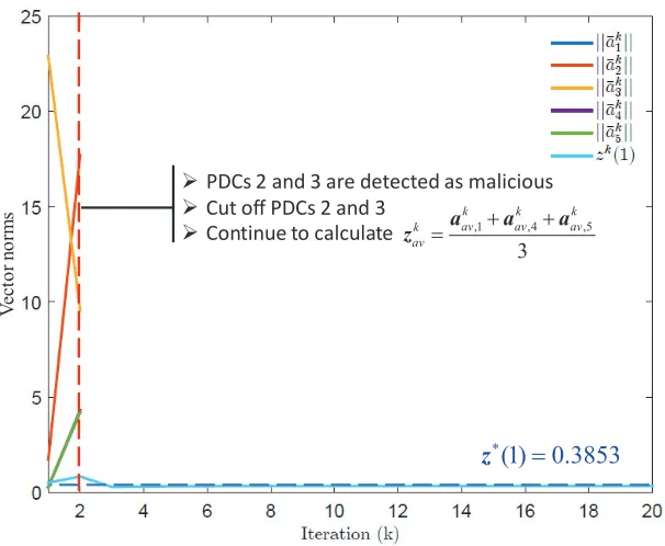
We illustrate the approach with a simple example. Consider a system with 5 local PDCs. The second and third PDCs are respectively injected with∆k2=δ2k1112n×1and∆k3=δ3k1112n×1, whereδ2k and δ3k are two different arbitrary time-varying numbers and 1112n×1 is a 2n×1 vector with all elements
one. All other PDCs are unbiased. Fig. 3.3 shows the first element of the consensus vectorzzzk before and after detecting the malicious PDCs uing Algorithm 1. In the figure, it can be seen that at iteration
k=2 we have||aaa¯21||=4.1864,||¯aaa22||=17.7189,||aaa¯23||=9.5428,||aaa¯24||=4.3161,||¯aaa25||=4.2459. Thus, ||aaa¯2max||=17.7189,||aaa¯2min||=4.1864, and||aaa¯2min2||=4.2459. The threshold, therefore, isγa2=0.2975. The estimates ¯aaa2are separated into three groups: ¯aaa21, ¯aaa24, and ¯aaa25are in the first group, ¯aaa22and ¯aaa23are in the second and the third groups, respectively. The magnitude||aaa¯21||in the first group is minimum. Thus, PDCs 1, 4 and 5 are identified as non-malicious, or alternatively, PDCs 2 and 3 are identified as malicious. After iteration 2, the central PDC cuts off communication with PDCs 2 and 3, and only calculates the average of messages received from the unbiased PDCs, leading tozzzk=13(aaak1+aaak4+aaak5),∀k>2. The estimates thereby asymptotically converge to the ideal solutionzzz∗, as expected.
3.2.3 Round-Robbin ADMM for Detecting the Malicious Users
ØPDCs 2 and 3 are detected as malicious ØCut off PDCs 2 and 3
ØContinue to calculate
z*(1)
=0.3853
V
ec
to
r
n
o
rm
s
,1 ,4 ,5
3
k k k
av av av k
av
+ +
=a a a
z
Figure 3.3: Evolution of the norms of the local estimates, and the averagezzzkbefore and after detection using S-ADMM. For convenience, we only show the first element ofzzzk.
Table 3.1: Comparison of S-ADMM and RR-ADMM for detection of attacks with large biases
S-ADMM RR-ADMM
Variable used for detection aaakav,j zzzkrr
Minimum # of computations per iteration N(N−2 1) 1 Minimum # of iterations needed to identify 1 kmin+N
Bias Magnitude Less stringent More stringent
want to track orkeep an eyeon a much smaller number of variables such as only the consensus vector
zzzkwhich has 2nnumber of elements in it. Under that condition, if any local estimateaaaki is corrupted by bias∆ki at every iteration, then it will be impossible for the central PDC to identify the malicious PDCs, or identify which PDCs are unbiased, just by trackingzzzk. The main question, therefore, is how can the central PDC catch the manipulators by simply trackingzzzkover every iteration? We next propose a variant of (2.15) using a Round-Robin strategy replacing the averaging step (2.15c) to solve this problem. We refer to this algorithm as Round-Robin ADMM or RR-ADMM in short.
receives local estimatesaaa1j from every local PDC, but computeszzz1simply aszzz1=αaaa11, whereα is a
constant non-zero number. Then the central PDC sends zzz1 back to the local PDCs following Step 4 of S-ADMM. Similarly, in iterationk=2, the central PDC useszzz2=αaaa22, at iteration k=3 it uses zzz3=αaaa33, and so on. In general,zzzk=αaaak((k−1)modN)+1.Nsuccessive iterations constitute oneperiod
of RR-ADMM whereN is the total number of local PDCs. AfterN iterations, the central PDC will again start from PDC 1, then PDC 2, and so on. For convenience of expression, we denote the consensus variables of RR-ADMM and S-ADMM at iterationkaszzzkrrandzzzkav, the latter being updated in (2.15c). Similarly, the local PDC estimates and its dual variable will be denoted asaaakrr,jandwwwkrr,j, andaaakav,j as in (2.15b) andwwwkav,j as in (2.15a), 1≤ j≤N, respectively.
Remark: Note that the purpose of using RR-ADMM is only to detect the malicious local PDC, not for obtaining the optimal solution of (2.14). This is because this algorithm is run by the central PDC stealthily, while every local PDC still believes that the central PDC uses S-ADMM to calculatezzzk, and thereby updatesaaakrr+,j1in the same way as in (2.15b). Therefore, this algorithm should be treated more as a S-ADMM with a RR-averaging step, rather than a true RR-ADMM where every step of (2.15) would have to be modified in accordance to the RR strategy.
Considering some of the PDCs to be malicious, the ADMM update equations using RR-averaging can be written as:
wwwkrr,i=wwwrrk−,i1+ρ(aaakrr,i−zzz k
rr), (3.9a)
a a
akrr+,i1=((HHHˆik)THHHˆki+ρIII)−1((HHHˆki)Tcccˆki −wwwki +ρzzzkrr), (3.9b)
alternative algorithm that applies for multiple attacks.
From (3.9), at iterationk, we can write the consensus vectorzzzkrras
zzzkrr=α∆kb+α
(HHHˆk−b 1)T(HHHˆk−b 1) +ρIII2n −1"
(HHHˆk−b 1)Tcccˆbk−1−www0rr,b−ρ
k−1
∑
j=1
(aaarrj,b−zzzrrj ) +ρzzzk−rr1 #
,
(3.10)
where b= ((k−1)modN) +1. We assume that the minimum absolute value of the element in the variable∆kbis large enough. It follows from (3.10) that the minimum value of||zzzrr||in one period must be from a non-malicious PDC. Letkmindenote the iteration index in the periodk=1, . . . ,Nwhere the magnitude of||zzzkrr||is minimum, 1≤k≤N, and define a thresholdγzas
γz=||zzzkrrmin+N|| − ||zzz kmin
rr ||. (3.11)
If||zzzkrr||>||zzzkmin
rr ||+γz,kmin≤k≤kmin+N−1, then the central PDC infers that the[(k−1)modN+1]th PDC is attacked. Algorithm 2 summarizes this detection mechanism.
Notice that if the biases are constant, the central PDC does not need to search for the minimum value of||zzzkrr||, 1≤k≤N, and the thresholdγzcan be defined as||zzzNrr+1|| − ||zzz1rr||. In that case, the central PDC will only wait forN+1+k∗iterations, notkmin+Niterations.
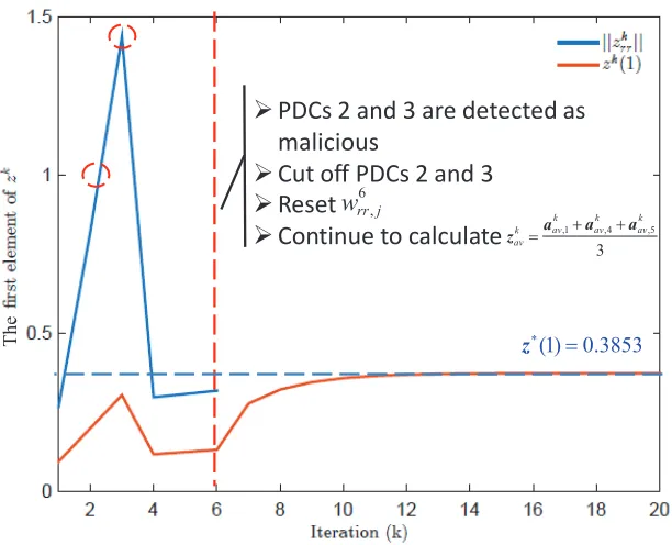
Consider the same example as in Fig. 3.3. Fig. 3.4 shows the first element of the consensus vectorzzzkrr
before and after detection using RR-ADMM. In the first period,||zzz1rr||=0.2672,||zzz2rr||=0.8192,||zzz3rr||= 1.4356,||zzz4rr||=0.2964, and||zzzrr5||=0.3064. Thus,||zzz1rr||is minimum andkmin=1. The threshold is computed asγz=||zzz6rr|| − ||zzz1rr||=0.0497. Only||zzz2rr||and||zzz3rr||are larger thanγz+||zzz1rr||. So PDCs 2 and 3 are identified as malicious. After detecting these manipulators at iteration 6, the central PDC cuts off the signal from PDCs 2 and 3, and only calculates the average of messages received from the other local PDCs leading tozzzkav=13(aaakav,1+aaakav,4+aaakav,5),∀k>6. Note that at the same time the dual variable
w
wwkj must be reset to its initial value. At iteration 7,aaa7av,j is updated using the value ofzzz6rr.
Algorithm 2Identifying malicious PDC with general biases using RR-ADMM
Detection:
1) At any iterationk, every local PDC computesaaakj+1in (2.15b) andwwwkj in (2.15a), j=1, . . . ,N, and transmits these two messages to the central PDC.
2) If at any iterationk∗>0 the central PDC finds N1 N ∑ i=1
wwwki∗−1
N N ∑ i=1
wwwki∗−16=0002n×1, it suspects that there
exists one or more malicious PDCs in the system.
Identification:
3) If Step 2 is positive, fork>k∗the central PDC switches to RR-ADMM. That is, every local PDC computesaaakrr+,j1in (3.9b) andwwwkrr+,j1in (3.9a), j=1, . . . ,N, and transmits them to the central PDC. 4) When k≥N+k∗, the central PDC searches for the minimum value||zzzkmin
rr ||in one period and its iteration indexkmin.
5) Waiting tillk≥kmin+N, the central PDC computes the thresholdγz=||zzzkrrmin+N|| − ||zzzkrrmin||. It then compares||zzzirr||to||zzzkmin
rr ||+γzforkmin≤i≤kmin+N−1. 6) If||zzzirr||>||zzzkmin
rr ||+γz, then the central PDC identifies the[(i−1)modN+1]
th
PDC to be malicious. 7) The central PDC repeats this classification for a few iteration, say up to iterations. If the identified non-malicious PDCs are consistent through these iterations, it finally confirms that these PDCs are unbiased.
8) Onwards from iterations+k∗, the central PDC ignores any message coming from the malicious PDCs, and simply carries out S-ADMM with the remaining non-malicious PDCs using (2.15). The final solution of this S-ADMM will lead to the solution of (2.14) as the LS problem is convex withs+k∗ being an initial iteration for the rest of the non-malicious S-ADMM.
dependent on the speed of divergence of the elements ofzzzrr in one period. For S-ADMM, however, ¯
a
aakav,j, 1≤ j≤N, are compared only at one iteration, and so the biases are less affected by the speed of divergence. Also note that if every element of the bias vector at every iteration is non-zero, and the central PDC knows this information, then the detection can be done by only using any chosen element of
¯
a
aakav,j, 1≤ j≤2n, andzzzkrr(for S- and RR-ADMM respectively) instead of using the vector norms. Table 3.1 compares S-ADMM and RR-ADMM for detecting attacks with large magnitudes.
3.2.4 Random Order of RR-ADMM
Ø
PDCs 2 and 3 are detected as
malicious
Ø
Cut off PDCs 2 and 3
Ø
Reset
Ø
Continue to calculate
av,1 av,4 av,53
k k k
k av
+a +a z =a
6
rr,j
w
z*(1)
=0.3853
The
Figure 3.4: Evolution of the averagezzzkbefore and after detection using RR-ADMM. For convenience, we only show the first element ofzzzk.
the second, (2, 4, 3, 1) for the third, and so on. This gives the central PDC the flexibility in choosing
zzzkrrin case any of the local estimates do not arrive on time due to message loss or denial-of-service. In that case, Algorithm 2 needs to be modified slightly to accommodate this random order. After Step 4 in Algorithm 2, the central PDC should find the index of the local PDC corresponding to the iteration index
kmin. Let this PDC index bem. Let ˜kbe the iteration index betweenN+1+k∗and 2N+k∗, considering
zzzkrr˜ =αaaa¯krr˜,m. The threshold is then changed toγz=||zzzkrr˜|| − ||zzzkrrmin||. After that the central PDC compares ||zzzkrr||toγz+||zzzkrrmin||, 1+k∗<k<N+k∗. If||zzzrrk ||>γz+||zzzkrrmin||and ifzzzrrk =αaaa¯krr,i∗, then thei∗thPDC is identified as malicious.
3.3
Data Manipulations with Small Biases
3.3.1 S-ADMM for Detecting Malicious Users with Small Biases
The basic approach for this method is the same as in Subsection 3.2.2. Recall equations (3.3) and (3.4) as follows. Fori∈S and j∈/S
d
ddki,+j1= (LLLi−LLLj)aaa˜k+ (PPPi−PPPj)∆k+∆ki+1, (3.12) ifi,j∈/S, then
d
ddki,+j1= (LLLi−LLLj)aaa˜k+ (PPPi−PPPj)∆k= (LLLi−LLLj)aaa˜k+ρ(Ai−Aj)∆k, (3.13) where the last equation follows from the definition ofPPPin Section 3.1. The problem, however, is that if ||∆ki+1||∞ is small, then the value of||ρ(Aj−Ai)∆k+∆ki+1||in (3.12) may become comparable to ||ρ(Ai−Aj)∆k||in (3.13), thereby leading to incorrect classification. One way to bypass this would be to reduce the value ofρ>0 such that the difference between the LHS of (3.12) and (3.13) is still large enough for detection despite||∆ki+1||∞being a small number. Thus, the only difference of this approach from that in Section 3.2.2 is that the ISO must ask every local PDC to reduce their penalty factorρonce
it realizes the presence of a false-data injector. Algorithm 3 describes this method.
Notice that the penalty factorρ is a private parameter, and hence unknown to the attacker. However,
following the attack model stated in Section 3.1, the communication link connecting the central PDC to any of the local PDCs, is assumed to be uncompromised. Thus, when the central PDC broadcasts the instruction to reduceρ, then every PDC whether attacked or unattacked, must be able to follow this
instruction. This satisfies Step 4 of Algorithm 3.