DOI: 10.1534/genetics.105.041368
Maximum-Likelihood Methods for Detecting Recent Positive Selection and
Localizing the Selected Site in the Genome
Haipeng Li
1and Wolfgang Stephan
Section of Evolutionary Biology, Department of Biology II, University of Munich, 82152 Planegg-Martinsried, Germany Manuscript received February 1, 2005
Accepted for publication June 9, 2005
ABSTRACT
Two maximum-likelihood methods are proposed for detecting recent, strongly positive selection and for localizing the target of selection along a recombining chromosome. The methods utilize the compact mutation frequency spectrum at multiple neutral loci that are partially linked to the selected site. Using simulated data, we show that the power of the tests lies between 80 and 98% in most cases, and the false positive rate could be as low as10% when the number of sampled marker loci is sufficiently large ($20). The confidence interval around the estimated position of selection is reasonably narrow. The methods are applied to X chromosome data ofDrosophila melanogaster from a European and an African population. Evidence of selection was found for both populations (including a selective sweep that was shared between both populations).
R
ECENT positive selection can be detected because it leaves footprints in the genome around the sites of selection. For instance, positive selection leads to a reduction of genetic diversity around the selected locus due to genetic hitchhiking (MaynardSmithand Haigh 1974), an excess of rare variants (Fuand Li1993), and an excess of mutations at high frequency (Fay and Wu 2000). On the basis of these effects, several efforts have been undertaken to detect recent positive selection (Fay and Wu2000), and some methods have been developed to estimate the parameters of simple models of genetic hitchhiking (Kim and Stephan 2002; Przeworski 2003).Here two exact-likelihood methods for detecting strongly positive selection and estimating the position of the selected site along a recombining chromosome are proposed, both of which are based on the combined effects of a local reduction of genetic variation and an excess of rare mutations. These methods go beyond the recently proposed composite likelihood-ratio tests of Kimand Stephan(2002) and Kimand Nielsen(2004) that treated each polymorphic site independently. Our approaches also differ from thead hocmethod of Sabeti
et al.(2002), who analyzed the decay of haplotype struc-ture around a selected locus.
The identification of genes contributing to the adap-tation of local populations is of great biological interest (Harret al.2002; Storzet al.2004). Thus our primary goal is to map these genes to a reasonably small DNA seg-ment by detecting selective sweeps in the genome. We do not focus on the estimation of the other parameters
of the hitchhiking model, i.e., the selection strength (a¼2Ns) and the time of the hitchhiking event in the past (t), wheresis the selection coefficient andNthe effective population size. Instead, to make the methods practicable, we opted to assign values to these two pa-rameters (these values may be obtained by different methods). Extensive simulations show that the estima-tion of the posiestima-tion of the selected locus is unbiased when the selected site is at the center of the region, and the tests are robust even when the true and as-signed values of the hitchhiking model differ to some extent.
METHODS
Coalescent simulation: Extensive coalescent simula-tions are needed to construct the ancestral recombina-tion graph for large DNA segments (Hudson 1990; Griffithsand Marjoram1997; Liand Fu1998; Wiuf and Hein 1999). Let us consider m neutral loci such that there is no recombination within a locus; thus each locus is treated as a point in the ancestral recombination graph. This assumption is reasonable because large DNA segments are considered such that the distance between marker loci and the selected site is large relative to the length of the loci. This procedure makes the simulation for large DNA segments (in the order of hundreds of kilobases) practicable since it is not needed to trace each nucleotide site.
The positions of these neutral loci were determined by two different ways. First, they were distributed ran-domly within a certain region. This strategy is called locus position strategy 1 (LPS1). Second, denote the region by [0,w). It is divided intomequally large seg-ments, and there is only one neutral locus per segment. 1Corresponding author: Department of Biologie II, LMU Mu¨nchen,
Grosshaderner Strasse 2, 82152 Planegg-Martinsried, Germany. E-mail: [email protected]
The position of the locus in the ith segment is distri-buted uniformly over [(i1)w/m,iw/m); thus it is also independent of the positions of the other neutral loci. The positions of loci tend to be uniformly distributed. This strategy is denoted as locus position strategy 2 (LPS2). The assigned selection strength and the time of the hitchhiking event in the past are ˆa(¼2N^s) and ˆt, respectively, where^sis the assigned selection coefficient. To plot the results obtained from the simulated data in physical distance rather than genetic distance, we assume that the recombination rate is 1 cM/Mb in the DNA segment under study (which is appropriate for Drosophila), and the population has a constant effective sizeN.
Denote the present time (when a population is sam-pled) as zero. Then, looking backward in time,t repre-sents the time in units of 2Ngenerations before present. The ancestral recombination and coalescence history is divided into three phases, the first neutral phase, the se-lective phase, and the second neutral phase (Braverman
et al.1995). Assuming the fixation time of the selected allele ists, the first neutral phase is [0,t), and the
se-lective phase is ½t;t1tsÞ, and the second neutral
phase is½t1ts;‘Þ, where tis the time of the fixation
event in the past.
The selective phase is the period when a beneficial mutation that causes a hitchhiking effect is on the way to fixation. The beneficial allele B has a genic selective advantagesover the parent alleleb. The allele frequency ofB, which is denoted asx, may be assumed to change deterministically from 1ctocif the population size is large and selection is strong; e.g., a¼2Ns is large (typically 103# a #23102N; Kaplan et al. 1989). Thenxat timetis given by
xðtÞ ¼ c
c1ð1cÞeaðttsÞ ð0#t#tsÞ ð1Þ (Stephanet al. 1992), where ts¼ ð2=aÞlnðcÞ, which is the length of the selective phase. We usec ¼1/2N
for the simulations. The coalescent and recombination probabilities follow previous work (Braverman et al. 1995; Kimand Stephan2002).
Likelihood method: The mutation rate of the kth neutral locus ismkper generation, anduk¼4Nmk. The
number of sampled chromosomes isn, wheren$5. Let jidenote the number of mutations that are oni chromo-somes. For example,j1is the number of mutations that are observed on one chromosome, andj2is the number
of mutations that occur on two chromosomes. Further-more, we havejX ¼Pn1
i¼3 ji. Then the compact
muta-tion frequency spectrum overmloci is defined as
D¼
j11; . . .; j1k; . . . ; j1m j21; . . .; j2k; . . . ; j2m jX1; . . .; jXk; . . . ; jXm
2 4
3 5:
jX represents the high-frequency mutations when sam-ple size is small. In this approach, some information,
like ‘‘branching information’’ indicating where the mutations happened and which size they are, has been partially discarded. The strategy has advantages, in particular when recombination is considered. In prac-tice, most randomly sampled genealogies are not con-sistent with the sequence data when the sample size is sufficiently large, and the failure rate can be.99.99%. An example is shown in Figure 1.
Using the compact mutation frequency spectrum, however, allows us to sample genealogies effectively. The probability is 1 that a genealogy has at least one internal branch with size$3 whenn$5. Then, a uniform sam-pling strategy can be used, and each random genealogy is consistent with the data. This sampling strategy is different from both importance sampling (Griffiths and Tavare´1994) and the Markov chain Monte Carlo method (Kuhneret al.1995).
Then, following Felsenstein and his colleagues (Felsenstein1992; Kuhneret al.1995), the probability that D is observed given the position of selected site (M) is
L¼PðDjMÞ ¼X
G
PðDjGÞPðGjMÞ; ð2Þ
whereG¼ ½G1;. . .;Gk;. . .;Gm, andGkis the
geneal-ogy for thekth locus. We also mention here thatMcould be a set of parameters, for example, the position of selected site, the strength of positive selection, and the time of fixation of the favored allele. In this study, we generally denoteHdiscrete candidate positions of the selected site as
M¼ ½M1;. . .;MH:
Then we need to compute the likelihood function
Li ¼PðDjMiÞfor a given value ofMi, to find the value
ofMithat maximizesL.
Since it is impossible to obtain an analytical expres-sion for the likelihood function, a simulation approach is proposed. Equation 2 requires a summation over a huge number of topologies, and each topology has an infinite number of possible branch lengths. Therefore, rather than sampling all genealogies, we consider a large Figure1.—High rejection rate of genealogies when a full
mutation frequency spectrum is considered. One mutation (A/T) of size 3 was observed in four sequences. There are two types of rooted topologies for four sequences. Of the two types, only the second one can explain the data be-cause it has a branch of size 3. Therefore, 33.3% (Tajima
random sample of G. The approach is possible and efficient because each simulatedGis consistent with the compact mutation frequency spectrum overmloci (D) whenn$5. SinceP(GjM) is determined in the simula-tion process (condisimula-tioned on the parameter set M), an estimate of L can be obtained by the following procedure:
1. Simulate genealogies (topology without mutation) formloci conditioned on the position of selected site (M), ˆaand ˆt.
2. Compute the value ofLGas
LG¼PðDjGÞ ¼
Ym
k¼1
Pðj1kjGkÞPðj2kjGkÞPðjXkjGkÞ;
wherePðjijGÞis given by the Poisson probability,
PðjijGÞ ¼l
ji
el
ji! ;
with l¼liu=2 and li as the length of the branches
with sizei, andlX ¼ Pn1
i¼3 li. The length of the branches
is scaled such that 1 unit represents 2Ngenerations. 3. Repeat steps 1 and 2 K times. Then L^ ¼ ð1=KÞ3
P
GLG.
Obviously, the accuracy of the estimation is improved by using large values of K. In the following, this procedure is denoted by L1. In addition, we propose a similar procedure, L2, as follows. The K simulations conditioned onM, given ˆaand ˆt, are used to calculate the average branch lengthlij, wherei¼1, 2,X, andj¼
1, 2,. . .,m. Then these average lengths are used to calculateL^according to a minor modification of step 2. The composite-likelihood method of Kim and Stephan(2002) (henceforth called KS) can be com-pared with L1 and L2. However, a minor revision is needed because the KS method is designed for contin-uous sequences under the infinite-site model. In this study, it is assumed that a locus in the KS model is composed of 300 nucleotide sites, and each nucleotide site within the locus has the same recombinational distance to the selected site, and there is no recombi-nation within the loci.
The likelihood-ratio test (LRT) is a statistical test of the goodness-of-fit between two models. Neutrality can be seen as a special case of hitchhiking, namely that the selected site is far away from the considered region such that there is no hitchhiking effect observed within the region. Hence, limM/‘LM ¼Lneutrality. Therefore,
one parameter is restricted in the neutral model on the basis of the hitchhiking assumption, and thus these two models are hierarchically nested. Then, we have x2¼ 2 lnðL
neutrality=LmaxÞ, and this LRT statistic
ap-proximately follows a chi-square distribution with 1 d.f., whereLneutralitycan be estimated by procedures similar
to L1 and L2, and Lmax is the maximum-likelihood
value under the hitchhiking model calculated by the method L1 or L2.
RESULTS
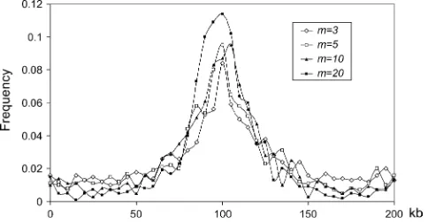
The parameters a or t can be estimated by the methods of Kimand Stephan(2002) and Przeworski (2003) or simply assigned by the following procedure. For a fixed value of the recombination rate, the length of the chromosomal region affected by a single hitchhik-ing event depends primarily on the strength of selection (Figure 2). A large region is affected when selection is strong, and thus the assigned strength of selection ˆa should be adjusted according to the length of the region when the selection strength is unknown. Assume that a selected site is at the center of the region and a neutral locus is at the edge of window. Let hbe the expected relative heterozygosity after a single hitchhiking event (i.e., the ratio of expected heterozygosity under hitch-hiking to that under neutrality), which is given by Equation 19 of Stephanet al.(1992) or Equation 3 of Kim and Stephan (2000). Then ˆa is the selection strength that makes the expected relative heterozygosity equal to the chosenh. We recommend to choose the size of the region such that 0.7 # h # 0.95. The effect of hitchhiking will be erased whentincreases. Therefore, it is expected that we have low power to detect these events if they happened some time ago. Thus, ˆt¼0 is recommended and used in this study.
log10L is depicted for a single simulated data set in Figure 3. The compact mutation frequency spectra were recorded at 10 loci, the positions of which were chosen randomly according to the LPS1 method. The selected site was at 100 kb when simulating the polymorphic data set. To estimate the position of the selected site by L1, it was assumed that selection must have happened within the 200-kb region, and the discrete candidate positions of the selected site were placed uniformly within the region. In this case, the space between two neighboring candidate positions is 5 kb. Discrete positions were used Figure 2.—The effect of positive selection with different
here because of the limit of computation power.L1can
be calculated by the method L1 when assuming that selection happened at the first candidate position. Thus,
L1,L2,. . ., can be calculated.L22is the global
maximum-likelihood value in this example, and the corresponding position is 105 kb.Lneutralcan be obtained by a similar
procedure based on simulations of the standard neutral model. Since the likelihood-ratio test rejected the standard neutral model in this example, selection was correctly detected. When the data created under the standard neutral model are considered, the neutral model could be falsely rejected by the likelihood-ratio test, which means a false positive.
Let us consider a certain region and assume that selection occurred at the center of the region. Then, what is the standard deviation of estimated position of the selected site given randomly selected samples and loci? The standard deviation of the estimated target position of selection is given in Table 1 and Figure 4
when a and t are known (namely, a¼aˆ ¼1000 and t¼ˆt¼0). The estimated position of the selected site is unbiased in all situations (results not shown). It is obvious that the more neutral marker loci are surveyed, the more precise the estimation becomes. Generally, the KS method (Kimand Stephan2002) performs similarly or slightly better than L1 and L2 when the number of neutral loci is small (m,10). L1 has a larger standard deviation than L2 and KS when the number of loci is large (m.10). L2 behaves best when the number of loci is not small (m.5) due to the lowest standard deviation. Overall, the power of both tests is so high that most of simulated hitchhiking events have been detected cor-rectly. The false positive rate decreases with an increas-ing number of loci. It should be important to lower the false positive rate unless it is known that positive selection has occurred within the region considered or unless positive selection events happen very frequently. We suggest that the number of neutral loci should be 10–20 or more in the region considered.
If the selected site lies at the center of the region, the estimated position of the selected site is always unbiased even if the distribution of the estimated position is uniform. Therefore, we also considered the cases that the target of selection is located at the edge of the region (Table 2). Generally, L1 and L2 are less biased than the KS method, and the more neutral marker loci are surveyed, the less biased the estimation becomes. Moreover, when the selected site lies at the edge of the region rather than at the center of the region (Table 1), standard deviation is larger and the power smaller.
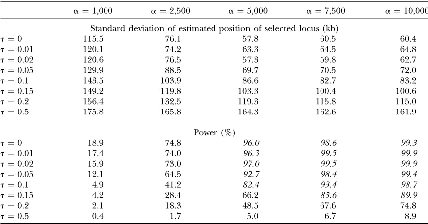
Usually the strength of selection and the time of the hitchhiking event in the past are unknown. Table 3 gives the effect of the difference between the assigned or estimated parameter values (ˆa and ˆt) and the true values (aandt). The results suggest that the proposed methods can reveal most selection events (.82%) if the true strength of selection is equal to or greater than the assigned value (a $aˆ) and selection happened very Figure3.—Illustration of the log-likelihood curve for one
simulated data set with a positive selection event occurring at 100 kb. The estimated position of the selected site is at 105 kb. N¼100,000,n¼10,m¼10,uk¼5,K¼1000, ˆa¼a¼1000,
and ˆt¼t¼0. The positions of the neutral loci are shown at the bottom.
Figure4.—The distribution of the estimated position of
se-lection (from 1000 simulated data sets). Parameter values are the same as in Figure 3, and the positions of themneutral loci in 1000 simulated data sets have been chosen according to method LPS1.
TABLE 1
The standard deviation (SD) of the estimated position of the selected locus, the power of the tests, and the false
positive rates
SD (kb) Power (%)
False positives
(%)
m KS L1 L2 L1 L2 L1 L2
3 42.0 43.0 44.0 72.8 87.6 20.0 36.8
5 37.8 38.4 36.3 93.6 93.4 41.4 38.7
10 31.0 33.8 29.8 96.7 97.4 26.9 28.0
20 23.0 28.7 20.2 93.0 97.6 7.8 11.4
The parameter values aren¼10,uk¼5,a¼aˆ¼1000, and
ˆ
recently (t,0.15). The methods will fail ifa>aˆ and t $0.5.
This suggests that a minimum strength of selection is detectable given the data. A large number of loci is required to obtain a low false positive rate, for example, 5%, and thus the size of the region cannot be reduced indefinitely. Therefore, ˆaand the minimum detectable value ofacannot be too small.
Furthermore, it is possible to study the power or the probability of detecting a selection event given that the beneficial allele (with the selection strengtha) fixed at timet, wheretis uniformly distributed between [t0,t1].
Whenais known and the assigned selection strength is ˆ
a, the probability is given by
Pða;aˆ;t1;t0Þ ¼
ðt1
t0
POWða;aˆ;tÞdt=ðt1t0Þ; ð3Þ
where POWða;aˆ;tÞ, the power given the beneficial allele fixed at the specified timet, can be obtained by simulation. When a is unknown but a.a, we haveˆ
Pða;aˆ;t1;t0Þ.Pðaˆ;aˆ;t1;t0Þ because we have
empiri-cally POWða;aˆ;tÞ.POWðaˆ;aˆ;tÞ(Table 3).
Next we consider different ways to choose the neutral loci (Figure 5). The LPS2 method generates less stan-dard deviation than LPS1 in all comparisons. This is because the positions of neutral loci chosen according to LPS2 are more likely to be equally distributed than those of LPS1, and thus the former contains more in-formation on the spatial distribution of polymorphisms. Thus, to increase the chance of detecting the hitchhik-ing event, it is recommended that, if possible, the marker loci should be equally or nearly equally distributed along the chromosome or within candidate regions.
In practice, the sequencing load is often a limiting factor. The more loci are chosen, the less base pairs per locus can be sequenced, and vice versa. Figure 6 displays the effect of the different choices. All comparisons show clearly that the first strategy (solid box) is better than the second one (open box). Therefore, we recommend that the priority should be put on the number of loci. By increasing the sequenced length per locus, more segre-gating sites are expected, so a more precise estimation of the level of local polymorphism can be obtained. However, Figure 6 shows that obtaining more informa-tion on the spatial distribuinforma-tion of polymorphisms along
TABLE 2
The standard deviation (SD) of the estimated position of the selected locus, the power of the tests, and the false
positive rates
Average estimated
position (kb) SD (kb) Power (%)
False positives
(%)
m KS L1 L2 KS L1 L2 L1 L2 L1 L2
3 66.8 58.9 61.0 62.6 60.3 63.4 52.3 68.8 21.8 39.9 5 57.3 49.9 47.8 57.5 55.9 58.9 80.4 81.8 42.5 37.9 10 45.1 33.7 29.0 50.4 49.8 47.6 84.8 85.9 28.2 25.6 20 34.6 18.3 19.6 43.6 34.4 36.6 77.2 89.9 6.4 8.9
The parameter values are the same as in Table 1, and the selected site is at the left edge of the region.
TABLE 3
The effect of the difference between assigned (aˆ andtˆ) and true (aandt) values of the model parameters
a¼1,000 a¼2,500 a¼5,000 a¼7,500 a¼10,000
Standard deviation of estimated position of selected locus (kb)
t¼0 115.5 76.1 57.8 60.5 60.4
t¼0.01 120.1 74.2 63.3 64.5 64.8
t¼0.02 120.6 76.5 57.3 59.8 62.7
t¼0.05 129.9 88.5 69.7 70.5 72.0
t¼0.1 143.5 103.9 86.6 82.7 83.2
t¼0.15 149.2 119.8 103.3 100.4 100.6
t¼0.2 156.4 132.5 119.3 115.8 115.0
t¼0.5 175.8 165.8 164.3 162.6 161.9
Power (%)
t¼0 18.9 74.8 96.0 98.6 99.3
t¼0.01 17.4 74.0 96.3 99.5 99.9
t¼0.02 15.9 73.0 97.0 99.5 99.9
t¼0.05 12.1 64.5 92.7 98.4 99.4
t¼0.1 4.9 41.2 82.4 93.4 98.7
t¼0.15 4.2 28.4 66.2 83.6 89.9
t¼0.2 2.1 18.3 48.5 67.6 74.8
t¼0.5 0.4 1.7 5.0 6.7 8.9
The effect is measured by the power of the test (with ˆa¼5000, ˆt¼0,m¼20, anduk¼5), where the window
the whole region is more important than getting more precise estimates of local levels of polymorphism.
Finally, we consider the case that the priority is given to the number of sampled chromosomes (n) rather than to the number of loci (m) (Figure 7). The priority given to the number of loci is the better strategy when the number of loci is not very large. This difference disappears when the number of loci gets large.
APPLICATION
The proposed likelihood methods were applied to a region on the X chromosome of D. melanogaster. The analyzed region extends over 660 kb. The region was selected due to the dense distribution of marker loci. This region contains 19 fragments that are nearly uni-formly distributed over the region (Figure 8). The data for seven of these loci are from Glinkaet al.(2003); the remaining data were kindly supplied by Lino Ometto and Sascha Glinka. On the basis of the published data (Glinkaet al.2003), the mean ofuacross the X
chromo-some in the European and African populations is 0.0044 and 0.0127 per site, respectively, so that the value ofufor each fragment is obtained as the mean value per site times the length of the fragment (excluding insertions and deletions). The estimated recombination rate is 3.8 cM/Mb (Glinkaet al.2003). The ancestral status of each polymorphic nucleotide site was determined by comparison with theD. simulanssequence (Glinkaet al. 2003).
To perform our analyses, the selection coefficient (^s) we assigned was 0.053, so thath, the relative heterozy-gosity, was 0.92 at the edge of the region. Moreover, we used ˆt¼0.
In the European population, the likelihood-ratio test via L1 and L2 rejected the standard neutral model in favor of the selective sweep model at the 5% level. It suggests that the observed polymorphism in the 19 par-tially linked fragments can be explained better by the hitchhiking model with the assigned^s- and ˆt-values than by the standard neutral model. In the African popula-tion, only the likelihood-ratio test via L2 rejected the standard neutral model.
In the European population, the positions of selected site estimated by L1 and L2 differ slightly. Both of them are between fragments 195 and 196 (the positions are 18.5 and 5.1 kb away from fragment 195, respectively). The 95% confidence regions of the positions estimated by L1 and L2 are shown in Figure 8. The 10,000 simulated data sets also show that the power of the tests is 96.3 and 97.5%, and the false positive rate is 11.3 and 15.7% for L1 and L2, respectively.
In the African population, the position of the selected site estimated by L2 is between fragments 196 and 197 (14.3 kb away from fragment 197), which is rather close to the positions estimated by L1 and L2 in the European population. The simulated data sets also show that the power of the test is high (97.7%) and the false positive Figure6.—Standard deviation of the estimated position of
the selected site for different sequencing strategies (m vs. length of marker locus). The solid bars represent the cases with more loci and a shorter sequence per locus. The open bars represent the alternative strategy (such that the sequenc-ing load in both cases is identical). Parameter values are the same as in Figure 3. LPS2 is used.
Figure7.—Standard deviation of the estimated position of
the selected site for different sequencing strategies (m vs. n). The solid bars represent the cases with fewer sampled chro-mosomes and more loci and the open bars the cases with more sampled chromosomes and fewer loci. Parameter values are the same as in Figure 3. LPS2 is used.
Figure5.—Standard deviation of the estimated position of
rate low (7.9%) for L2. The 95% confidence region of the position estimated by L2 is shown in Figure 8. It overlaps with those of the European population.
DISCUSSION
Method: In this study, two exact-likelihood methods are proposed. The methods are generally based on coalescent simulations using the ancestral recombina-tion graph. Furthermore, the compact mutarecombina-tion fre-quency spectrum is used to compute the likelihood.
In the proposed methods, L2 shows a lower standard deviation in the estimated position of selection than L1 in some cases because of the difference in dealing with branch lengths. There is a large variance of branch length in individual simulations in L1, while in L2 the variance is reduced by averaging the branch lengths. Furthermore, to understand this difference, let us con-sider the genealogies under hitchhiking for two loci with two sampled chromosomes. In some cases, there is no recombination between the two loci, so that the two branches will coalesce. And thus the distance between loci is not counted efficiently by the likelihood in L1. However, by averaging the branch length among simu-lations, a shorter average branch length will be observed
in the locus that is closer to the selected site, and thus the distance between loci is counted by the likelihood in L2. However, L1 also shows a lower standard deviation of the estimated position of selection than L2 in some cases. This is because information on correlations among loci is discarded in L2. Thus, both L1 and L2 are recommended in practice. For a given genomic region, the estimated positions of the selected site by L1 and L2 could be dif-ferent. In such a case, the variance of estimated position of the selected site can be obtained, and the method generating a lower variance should be used.
Unlike the Bayesian approach (Przeworski 2003), the proposed likelihood methods do not incorporate prior information about the model parameters. If we expect that beneficial mutations occur preferentially in coding and control regions, the Bayesian approach may be helpful.
A global sweep in D. melanogaster: In application, the two proposed methods were applied to 19 partially linked loci on the X chromosome ofD. melanogaster. The hitchhiking model was accepted for the assigned param-eters, and the position of the selected site (estimated by the various methods) falls into a 54-kb region. The divergence between D. melanogasterandD. simulans in this region is at the same level as the average divergence between the two species over the whole X chromosome (data not presented). Thus the deficiency of polymor-phism cannot be explained by a relatively low mutation rate. Given the fact that the hitchhiking model was accepted in both the European and African popula-tions, we suggest that a recent hitchhiking event may have occurred in the ancient African population. As the confidence intervals of the estimated positions overlap in the African and European populations, this selective sweep may have continued in the European population driven by the same selected allele. The sweep in Africa is likely to be older as levels of nucleotide diversity are higher than those in Europe. Thus we may have a global selected sweep. Alternatively, two independent local hitchhiking events have to be postulated, one in the European population and another in the African pop-ulation. These alternatives may be distinguished by mapping the positions of the selected sites more pre-cisely on the basis of more densely spaced marker loci. For the time being, a global sweep is the more parsimo-nious explanation.
In this study, we did not consider the effect of demography, such as population size bottlenecks and expansions. However, our approach can be extended to analyze populations with variable size. Finally, we note that the methods can also be used to estimate a and tafter minor revision, but it would consume much more computing time.
We thank David De Lorenzo, Sascha Glinka, and Lino Ometto for providing unpublished data and Joachim Hermisson and Sylvain Mousset for helpful discussions. This work was funded by the VolkswagenStiftung (grant I/78815).
Figure 8.—Genetic diversity ofDrosophila melanogaster
be-tween African and European populations. The dashed lines are the expected u-values for each population. (Top) Frag-ments are denoted according to their identification numbers (Glinkaet al.2003). (Bottom) Their positions on the X
LITERATURE CITED
Braverman, J. M., R. R. Hudson, N. L. Kaplan, C. H. Langleyand
W. Stephan, 1995 The hitchhiking effect on the site frequency
spectrum of DNA polymorphisms. Genetics140:783–796. Fay, J. C., and C.-I Wu, 2000 Hitchhiking under positive Darwinian
selection. Genetics155:1405–1413.
Felsenstein, J., 1992 Estimating effective population size from
samples of sequences: a bootstrap monte carlo integration method. Genet. Res.60:209–220.
Fu, Y.-X., and W.-H. Li, 1993 Statistical tests of neutrality of
muta-tions. Genetics133:693–709.
Glinka, S., L. Ometto, S. Mousset, W. Stephanand D. D. Lorenzo,
2003 Demography and natural selection have shaped genetic variation in Drosophila melanogaster: a multilocus approach. Genetics165:1269–1278.
Griffiths, R. C., and P. Marjoram, 1997 An ancestral
recombina-tion graph, pp. 257–270 inProgress in Population Genetics and Human Evolution, edited by P. Donnelly and S. Tavare.
Springer-Verlag, New York.
Griffiths, R. C., and S. Tavare´, 1994 Simulating probability
distri-butions in the coalescent. Theor. Popul. Biol.46:131–159. Harr, B., M. Kauerand C. Scho¨ ltterer, 2002 Hitchhiking
map-ping: a population-based fine-mapping strategy for adaptive mu-tations inDrosophila melanogaster.Proc. Natl. Acad. Sci. USA99:
12949–12954.
Hudson, R. R., 1990 Gene genealogies and the coalescent process,
pp. 1–44 inOxford Surveys in Evolutionary Biology, Vol. 7, edited by D. Futuyma and J. Antonovics. Oxford University Press,
New York.
Kaplan, N. L., R. R. Hudsonand C. H. Langley, 1989 The
‘‘hitch-hiking effect’’ revisited. Genetics123:887–899.
Kim, Y., and R. Nielsen, 2004 Linkage disequilibrium as a signature
of selective sweeps. Genetics167:1513–1524.
Kim, Y., and W. Stephan, 2000 Joint effect of genetic hitchhiking
and background selection on neutral variation. Genetics 155:
1415–1427.
Kim, Y., and W. Stephan, 2002 Detecting a local signature of genetic
hitchhiking along a recombining chromosome. Genetics 160:
765–777.
Kuhner, M. K., J. Yamato and J. Felsenstein, 1995 Estimating
effective population size and mutation rate from sequence data using Metropolis-Hastings sampling. Genetics 140:1421– 1430.
Li, W.-H., and Y.-X. Fu, 1998 Coalescent theory and its applications
in population genetics, pp. 45–79 inStatistics in Genetics, edited by E. Halloran. Springer-Verlag, New York.
MaynardSmith, J., and J. Haigh, 1974 The hitch-hiking effect of a
favorable gene. Genet. Res.23:23–35.
Przeworski, M., 2003 Estimating the time since the fixation of a
beneficial allele. Genetics164:1667–1676.
Sabeti, P. C., D. E. Reich, J. M. Higgins, H. Z. P. Levine, D. J.
Richter et al., 2002 Detecting recent positive selection in
the human genome from haplotype structure. Nature 419:
832–837.
Stephan, W., T. H. E. Wieheand M. W. Lenz, 1992 The effect of
strongly selected substitutions on neutral polymorphism: analytical results based on diffusion theory. Theor. Popul. Biol.
41:237–254.
Storz, J. F., B. A. Payseurand M. W. Nachman, 2004 Genome
scans of DNA variability in humans reveal evidence for selective sweeps outside of Africa. Mol. Biol. Evol.21:1800–1811. Tajima, F., 1983 Evolutionary relationship of DNA sequences in
fi-nite populations. Genetics105:437–460.
Wiuf, C., and J. Hein, 1999 Recombination as a point process along
sequences. Theor. Popul. Biol.55:248–259.