On the Selection of Time Series Representative of Site Specific Seismic Motion

On the selection of time series representative of site specific seismic motion

Catherine Berge-Thierry1, Julien Rey2 and Sylvain Lavarenne1

1 Nuclear safety and Radioprotection Institute, France. 2 Today at the Geological and Mine Research Survey.

ABSTRACT

The methodologies used for evaluating the stability of structures under seismic solicitation require accelerograms for computations. In the framework of the French nuclear power plants regulation (RFS V.2.g), the selection of accelerograms representative of the site-specific seismic motion was, up to now, based only on the fit to the deterministic target response spectrum. During the revision of this regulation last year, it was proposed to complete the selection:

- by targeting different significant seismic parameters other than spectral pseudo acceleration, such as seismic duration – SMD -, Arias Intensity – AI - and Cumulative Absolute Velocity – CAV - predicted by new empirical attenuation relations,

- and allowing the variation of these parameters using the standard deviation associated to the predictions.

This paper presents the procedure proposed for selecting natural as well as for generating synthetic accelerograms taking into account the variability observed in strong motion databases on seismic parameters such as PGA, Arias intensity, Cumulative Absolute velocity or duration.

INTRODUCTION

The presented work was motivated by the recent revision of the structural design French code for nuclear plants (ex RFSV.2.g [1]). Up to now, the seismic input was restricted to a deterministic spectrum (seismic hazard assessment for NPP called, RFS 2001-01 [2]) evaluated by a specific attenuation relationship derived from an essentially European strong motion database slightly modified after Berge-Thierry et al. 2003, [3]. These data show, in accordance with recent major earthquakes (Izmit 1999, Parkfield 2004 …), a strong intrinsic variability. Complex radiation source processes, wave propagation, attenuation phenomena and geological media heterogeneities are partly responsible for the variability and cannot be captured through a simple triplet model representation of [Magnitude/Event to site Distance/Geological site condition]. Then the RFS 2001-01 encourage to complete the response spectrum information, by others seismic parameters.

We then derived specific attenuation relationships for the PGA, the SMD, the AI and the CAV based on an extraction of the RFS 2001-01 strong motion database. Analysis of the residuals observed/predicted shows log-normal distributions covering different ranges from +/- 3 σ (PGA) to only +/-1 σ (SMD). Finally we propose a procedure to select natural accelerograms or to produce synthetics that account for the variability using these seismic parameters and their dispersion around the mean predicted values. We show the applicability of the procedure on natural and synthetic accelerograms.

STRONG MOTION DATABASE (SMDB)

As the aim of the study is to propose a coherence between the seismic hazard assessment code and the structural design one’s, we used the RFS 2001-01 strong motion database (SMDB). This database is the one presented in Berge-Thierry et al. 2003 [3], on which we performed a correction and applied some additional criteria on time series.

Correction of Imperial Valley data of the Berge-Thierry et al. 2003 database

around 20 km (illustrated on Figure 1). The standard deviation associated to the new database for predicting response spectrum is slightly improved. In the framework of the RFS application in France, we consider these differences as negligible (with respect to the standard deviation of the prediction). In the present work, we use this 989 records database, and associated coefficient regression for predicting response spectra.

Figure 1: Sensitivity of the results in terms of response spectrum prediction after correction of bad attribution of parameters for 7 stations recording the mainshock of 1979 Imperial Valley event, and adding 12 stations recording the Magnitude 5 Imperial Valley aftershock.

Exclusion of records non adapted for energy and duration parameters estimation

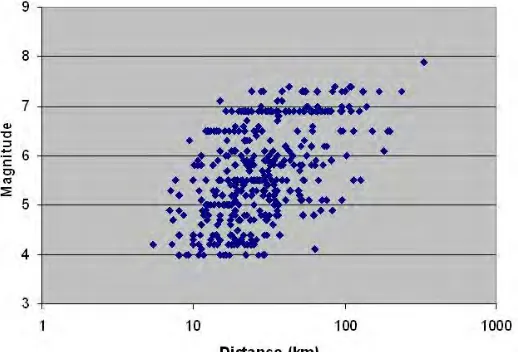
We carefully and visually checked the new database, composed by 989 records described above and excluded those for which the whole waveform (including the P wave’s arrivals) is not recorded. Indeed the estimation of parameters based on the strong motion duration requires complete recordings. Finally, the database for the present study is composed of 730 strong motions coming mainly from the European database published in Ambraseys et al., 2000 [5], with few Californian data to complete the magnitude distribution. Figure 2 summarizes the strong motion database used in this study, in the magnitude to site-to-event distance space.

Figure 2: Distribution in the distance and magnitude space of the 730 data selected in our database.

EMPIRICAL RELATIONSHIPS FOR SEVERAL SEISMIC INDICATORS, COMPLEMENTARY TO THE RESPONSE SPECTRUM

Attenuation relationships for predicting seismic parameters

displacement D (cm), the A/V (s-1) ratio, the mean frequency F (Hz), the dispersion around the mean frequency δ=dF/F, the strong motion duration T (s) defined variously (significant duration, Trifunac and Brady, 1975 [6], or the Uniform duration used in Bommer and Martinez-Peirera, 1999 [7], or the bracketed duration used in several studies Bommer and Martinez-Pereira, 1999 [7], Koutrakis et al., 2002 [8], Wang et al., 2002 [9]), the Cumulative Absolute Velocity CAV (m/s), and the Arias Intensity AI (m/s). In this study we finally retain 4 parameters complementary to the response spectrum already defined by in Berge-Thierry et al., 2003 [3], two parameters related to the released energy the CAV and the Arias Intensity, and a duration parameter. We choose the “significant duration” defined as the time interval Ds during which the Arias intensity reaches between 5% and 95% of the total energy (Arias intensity on the whole seismic record). We added the PGA (named Amax), parameter required for the generation of synthetic accelerograms using classical procedures.

Based on the strong motion database (SMDB, 730 signals), without considering the soil properties as a parameter, we derived attenuation relationships, based on the following model:

Log (Seismic Parameter) = a*M + b*R – Log(R) + c

where, M is the surface Magnitude, R the hypocentral distance, et Log is the 10 base logarithm. We then obtained the following three relationships for Amax , AI, CAV:

Log (Amax (cm/s 2

)) = 0.3112*M – 0.0009562*R – Log(R) + 1.591 (σ=0.2840) (1) Log (AI (cm/s)) = 0.7303*M - 0.007437*R - Log(R) + 0.3099 (σ=0.5068) (2) Log (CAV (cm/s)) = 0.4515*M – 0.001265 – Log(R) + 1.070 (σ=0.2611) (3)

For the duration parameter, referring the literature we selected the following attenuation model Log (Duration parameter) = a*M – b*Log(R) + c

Finally, the empirical prediction relationship for duration deduced from our database is: Log (T(s)) = 0.09408*M + 0.4834*Log(R) – 0.2453 (σ=0.2247) (4)

Testing the log normal distribution for each seismic parameter

In a second step we tested the accuracy of our model for predicting the data, and especially the hypothesis of a log normal distribution data. For this step we firstly applied a graphical test, named the “Henry’s graph” applied to our dataset three classical statistical tests (the Kolmogorov-Smirnov test, Jarque-Bera and Lilliefors tests that enable to estimate the behaviour of a dataset with respect to a perfect lognormal distribution).

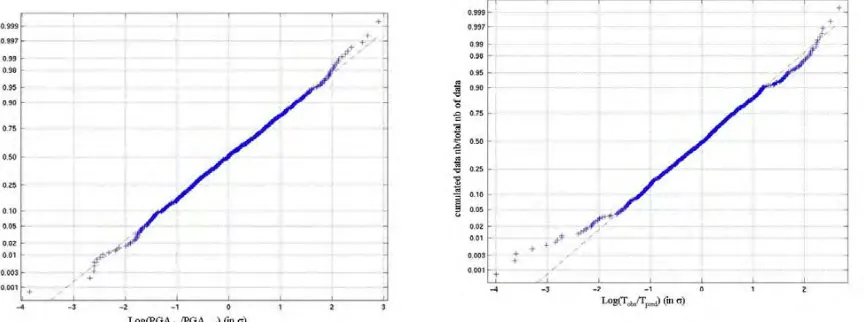
Figure 3 : Henry’s graphs for the PGA (left) and Duration (right) parameters. X axis shows the residual distribution in terms of number of sigma of the attenuation relationship. Y axis shows the number of cumulated data over the total number of data.

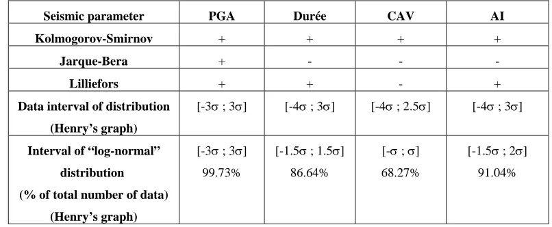
Figure 3 presents for the PGA and duration parameters the behaviour of the prediction using the attenuation relationships we proposed in previous section (equations (1) and (4)) with respect to the observed data. The deviation is measured in terms of number of standard deviation. Based on such graphs we extracted for each parameter the domain of distribution of the residuals (see table 1, last line), and we defined the domain on which the residual distribution is reasonably well predicted using the lognormal assumption (see table 1, fourth line). In addition to this visual determination based on Henry’s graphs, we performed three statistical tests on the distribution, whose results are summarized in Table 2 (where ‘+’ and ‘–‘ corresponds to a positive or negative test with respect to a log normal distribution assumption). From these tests the CAV appears to be the less constrained using the empirical attenuation relationship (confirmed by the last line of the table 1).

Table 1: Synthesis of the statistical tests with respect to a lognormal distribution. ‘+’ indicates a positive test result, ‘-‘ a negative on (lines 1 to 3). Distribution domains for the residuals between observed data and predicted data using the attenuation relationships (equation (1) to (4)), in terms of deviation to the mean (number of σ (lines 4 and 5).

Seismic parameter PGA Durée CAV AI

Kolmogorov-Smirnov + + + +

Jarque-Bera + - - -

Lilliefors + + - +

Data interval of distribution

(Henry’s graph)

[-3σ ; 3σ] [-4σ ; 3σ] [-4σ ; 2.5σ] [-4σ ; 3σ]

Interval of “log-normal”

distribution

(% of total number of data)

(Henry’s graph)

[-3σ ; 3σ]

99.73%

[-1.5σ ; 1.5σ]

86.64%

[-σ ; σ]

68.27%

[-1.5σ ; 2σ]

91.04%

SELECTING NATURAL ACCELEROGRAMS THAT FIT SEVERAL PARAMETERS IN THEIR VARIABILITY DOMAIN

Selection limited to a 1 σ interval around mean predicted values

The aim of this section is to quantify the number and repartition of records fitting simultaneously the following criteria for a target event characterized by (MT,dT):

First criterion

:

(MT-0.25)<M<(MT+0.25) and (dT-5)<dacc<(dT+5) or (dT-10)<d<(dT+10) for greater distances,

Criterion 2: Strong motion records whose the 4 seismic parameters studied here (i.e., PGA, duration, CAV, AI) fit the

mean predicted value (using equations 1 to 4) in a 1 σinterval,

Criterion 3: Strong motions records best fitting (in a least squares minimization) the response spectrum evaluated using coefficients provided in RFS 2001-01 [2].

Table 2 below presents the number and repartition in the magnitude and distance space of the data that respect the 3 criteria (the selection being performed in the RFS 2001-01, 965 records, database). The best constrain domain is the magnitude between 5 and 6 for moderate distance (from 10 to 60 km).

Selection widened to the lognormal interval of each parameter

The same selection has been performed but accounting for the domain where the distribution of data follows the lognormal behaviour. For each seismic parameter we then allow the parameter to fit the mean predicted value using the attenuation relation in a n*σ domain uncertainty (n being defined for each parameter in Table 1 last line). The selection procedure is the same than described below excepted for the second criterion that becomes:

Criterion 2: Strong motion records whose the 4 seismic parameters studied here (i.e., PGA, duration, CAV, AI) fit the mean predicted value in a n*σ interval, n being equal to 3, 2, 1.5 and 1 respectively (using equations 1 to 4).

Table 2 summarizes the results for the 2 selections. When considering the lognormal interval of each parameter (number of accelerograms indicated between brackets, table 2), the selection increases for certain (M and distance) bins with respect to the previous one (only 1σ around the mean), and allows to cover a broader magnitude and distance range.

Table 2 : Repartition by magnitude and distance bins of the selected data (fitting the 3 criteria described above: first selection with a search limited to 1σ around the mean, second selection indicated in brackets widened to the lognormal distribution domain –i.e. nσ - for each parameter). Selection performed in the RFS 2001-01, 965 records database.

Nb of selected

accelerograms 4.5<M<5.0 5.0<M<5.5 5.5<M<6.0 6.0<M<6.5 6.5<M<7.0 7.0<M d<10 4 (6) 2 (2) 1 (1) 1 (1) 0 (0) 0 (0) 10<d<20 20 (31) 24 (45) 12 (23) 8 (13) 8 (12) 2 (4) 20<d<40 5 (10) 12 (24) 15 (30) 7 (12) 10 (19) 2 (3) 40<d<60 0 (1) 8 (10) 10 (11) 4 (5) 9 (10) 0 (2) 60<d<80 0 (0) 0 (0) 2 (2) 0 (0) 2 (2) 2 (2) 80<d<100 0 (0) 0 (0) 0 (0) 1 (2) 4 (4) 2 (4)

Scheme of the proposed procedure for selecting natural accelerograms

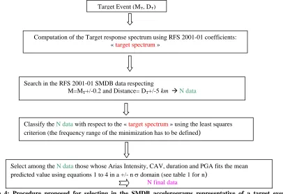
Based on the tests presented above, we propose the procedure illustrated by the flowchart for selecting in a database natural accelerograms representative of a target seismic event. The selection is not restricted to the fit to the target response spectrum but include the simultaneous fit of the target 4 other parameters (PGA, duration, CAV, AI) accounting for the variability of their prediction through empirical attenuation relationships.

Figure 4: Procedure proposed for selecting in the SMDB accelerograms representative of a target event , including the response response fit and the 4 seismic parameters (Arias Intensity, CAV, duration and PGA) accounting for their variability prediction through empirical attenuation relationships 1 to 4.

SYNTHETIC ACCELEROGRAMMS AND SEISMIC PARAMETERS VARIABILITY

Seismic parameters variability from synthetic accelerograms generated by “standard engineering codes” In this section we tested the performance of classical codes used by engineers (such as Castem, SIMQUAKE…) with respect to the natural seismic variability, through the 4 parameters described above. Limitations of such codes come from standard parameters: when it was possible we forced some parameters to be in agreement with our empirical predictions (strong motion duration for example). Using SIMQUAKE code, we computed a synthetic database (10 synthetics for each distance bin and each site class, i.e. 100 signals) in order to compare with. the original SMDB [730 data]. We then compare the variability of resulting seismic parameters with respect to the natural one. Figure 5 illustrates on the duration parameter the poor variability of synthetic data with respect to the observed one: this conclusion is also valid for the three other studied parameters (AI, PGA and CAV).

Target Event (MT, DT)

Computation of the Target response spectrum using RFS 2001-01 coefficients: « target spectrum »

Search in the RFS 2001-01 SMDB data respecting

M=MT+/-0.2 and Distance= DT+/-5 km ÆN data

Classify the N data with respect to the « target spectrum » using the least squares criterion (the frequency range of the minimization has to be defined

)

Select among the N data those whose Arias Intensity, CAV, duration and PGA fits the mean predicted value using equations 1 to 4 in a +/- n σ domain(see table 1 forn

)

Figure 5 : Comparison of strong motion durations from synthetic acelerograms generated by SIMQUAKE (red and blue circles) with respect to strong motion durations extracted from real data (of the SMDB [730 signals]) for various magnitude and distance distributions.

Seismic parameters variability from synthetic accelerograms provided by the Pousse et al., 2006 [10] modified code

In order to improve the quality of synthetic accelerograms with respect to their seismic variability representativity, we propose to adapt the procedure developed in Pousse et al, 2006 [10]. In this paper, these autors modified the original procedure of Sabetta and Pugliese in 1996 [11]. The two main modifications are the strong motion database on which the seismic parameters are calibrated (on a restricted Italian dataset originally, on a broad Japanese dataset in Pousse et al., 2006 [10]), and the introduction of the variability associated to the prediction of seismic parameters.

In this section, we adapted the procedure of Pousse et al., 2006 [10] to our database. We then use the following relations derived from the 730 strong motion database, established for the 2 site conditions (« rock » and « soil » as defined in Berge-Thierry et al., 2003 [3]):

Log (Amax (cm/s 2

)) = 0.3109*M – 0.0009966*R – Log(R) + 1.558 (rock) or + 1.605 (soil) (σ=0.2833) Log (T(s)) = 0.09074*M + 0.4989*Log(R) – 0.2839 (rock) or - 0.2373 (soil) (σ=0.2244)

Log (AI (cm/s)) = 0.7402*M – 1.808*Log(R) + 1.051(rock) or + 1.176 (soil) (σ=0.4987)

Other quantities are used in the Sabetta and Pugliese 1996 procedure, the « central frequency » Fc and the ratio Fb/Fc defined as the band width, whose behaviour are represented by following relationships:

Fc= a + b.ln(t), with a and b equal to:

« Rock » : a = -0.0196*M + 2.1465 et b = 0.0129*M – 0.2088 « Soil » : a = -0.0677*M + 2.4292 et b = 0.0299*M – 0.4437

Log(Fb/Fc) = 0.01902*M – 0.03510*Log(R) – 0.3081 (rock) or – 0.2635 (soil) (σ=0.1021)

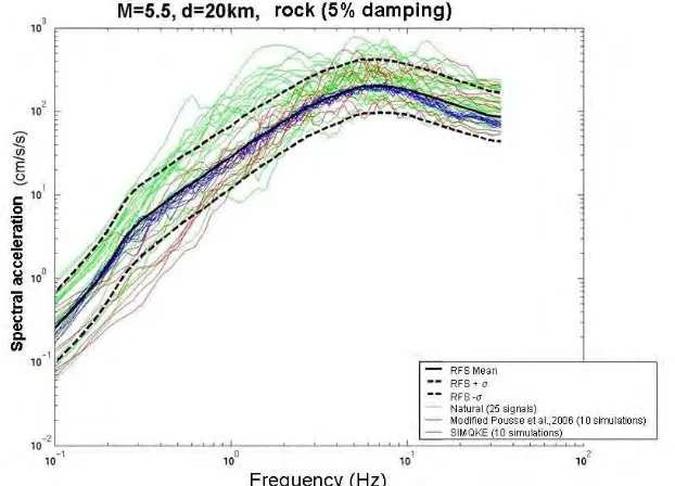
The algorithm proposed by Sabetta and Pugliese in 1996, [11] has been modified by Pousse et al. in 2006 [10] in order to include the dispersion around the mean value of all used parameters (AI, PGA, duration, Fc(t) ou Fb/Fc) : supposing that the distributions of these parameters are lognormal, an aleatory research is performed in the [-xσ,+xσ] around the mean, with x values being given in table 1 last line. We then reproduce the (M,distance) distribution data of the SMDB [730 data], as we did to test the signals generated using SIMQUAKE code. In this case, 3 of the 4 studied parameters are directly used in the code to construct the synthetics (CAV is not retained). Figure 6 illustrates the improvement of seismic variability on PGA parameter using the Pousse et al., 2006 [10] modified code. This improvement is also valid for other studied parameters. The synthesis of the work is given on Figure 7, for the response spectrum parameter, considering a (M=5,5 at 20 km, rock site) target triplet: the selection is performed using the procedure described on Figure 4.

Figure 6: Comparison of PGA from synthetic acelerograms generated by Pousse et al. (2006) code, adapted to our database (blue circles) with respect to PGA extracted from real data (of the 730 signals of the SMDB) for various magnitude and distance distributions.

Figure 7 : Acceleration spectra of real data (green curves) selected in our database versus synthetics generated using SIMQUAKE (blue curves) and synthetics using the Pousse et al. 2006 code adapted to our database (red curves). Black thick and dashed spectra are respectively the mean predicted by RFS 2001-01 attenuation relationship, and the +/- one σ.

CONCLUSION

The work presented is this paper has been discussed during the revision of the structural design code RFS V.2.g. The revised regulation, named GUIDE/ASN/2/01 [1], has finally adopted an accelerograms selection still based mainly on the response spectrum target criterion. However the agreement between the selected records and the magnitude and distance parameters associated to the target event is now required, while the fit to others seismic indicators as those we suggested (Arias intensity, motion duration …) is strongly encouraged.

The next step of this work will be to quantify the “acceptable” seismic variability regarding the structural seismic response. In this way, we propose to test this procedure to select the time series in the framework of a site specific probabilistic safety analysis.

REFERENCES

1. Guide ASN/2/01 (ex RFS V.2.g), « Prise en compte du risque sismique à la conception des ouvrages de génie civil d’installations nucléaires de base à l’exception des stockages à long terme des déchets radioactifs », 26 mai 2006. 2. RFS 2001-01, « Règle Fondamentale de Sûreté relative à la détermination des mouvements sismiques d’installations nucléaires de base », DSIN-GRE/SD2/n°79-2001, 16 mai 2001.

3. Berge-Thierry C., F. Cotton, O. Scotti, DA. Pommera and Y. Fukushima 2003. “New empirical response spectral attenuation laws for moderate European earthquakes”, Journal of Earthquake Engineering, Vol 7, n° 2, 2003, pp. 193-222.

4. Joyner W.B, and D.M. Boore, “Peak horizontal acceleration and velocity from strong-motion records including records from the 1979 Imperial Valley, California, earthquake”, Bull. of the Seism. Soc. of Amer., Vol. 71, n°6, 1981, pp. 2011-2038.

5. Ambraseys N.N., Smit P., Berardi R., Rinaldis D., Cotton F. and Berge C.; “Dissemination of European Strong- Motion Data”. CD-ROM collection. European Commission, Directorate-General XII, Environmental and Climate Programme, ENV4-CT97-0397, Brussels, Belgium, 2000.

6. Trifunac M.D. and Brady A.G., “A study on the duration of strong earthquake ground motion”, Bull. of the Seism. Soc. of Amer., Vol. 65, n°3, 1975, pp. 581-626.

7. Bommer J.J. and A. Martinez-Pereira, “The effective duration of earthquake strong motion”, Journal of Earthquake Engineering, VOL.3, n°2, 1999, pp. 127-172.

8. Koutrakis S.I., Karakaisis G.F., Hatzidimitriou, P.M. Koliopoulos, P.K. Margaris V.N, “Seismic hazard in Greece based on different strong ground motion parameters”, Journal of Earthquake Eng., Vol.6, n°1, 2002, pp. 75-109. 9. Wang G-Q, Zhou X.Y., Zhang P.Z. and Igel H., “Characteristics of amplitude and duration for near fault strong motion from the 1999 Chichi, Taïwan earthquake”, Soil dynamics and earthquake engineering, Vol 22, 2002, pp. 73-96. 10. Pousse, G., Bonilla, L.F., Cotton F., and Margerin, L. “Non Stationary Stochastic Simulation of Strong Ground Motion Time Histories Including Natural Variability: application to the K-net Japanese Database”, Bull. Seism. Soc. Of America, Vol 96 n°6, 2006, pp 2103 – 2117.

11. Sabetta A. and Pugliese A., “Estimation of response spectra and simulation of non stationary earthquake ground motions”, Bull. of the Seism. Soc. of Amer., Vol. 86, n°2, 1996, pp.337-352.