Perturbation Bootstrap in Regression.

(1)

Abstract

DAS, DEBRAJ. Perturbation Bootstrap in Regression. (Under the supervision of Pro-fessor Soumendra Nath Lahiri)

Consider the multiple linear regression model

yi = x′iβ+ϵi, i =1, 2, . . . ,n

wherey1, . . . ,yn are responses,ϵ1, . . . ,ϵn are independent errors,x1, . . . ,xn are design vectors and βis thep-dimensional vector of parameters. After introduction of pertur-bation bootstrap by Jin et al. (2001), the asymptotic properties of this method remains largely unexplored in the context of multiple linear regression. In this dissertation, we analyze the asymptotic properties of perturbation bootstrap method as a distribution approximation method for different estimators ofβ.

(2)

In chapter two, we consider sparsity in the underlying multiple linear regression model and subsequently investigate the asymptotic properties of perturbation boot-strap in case of Lasso. Least Absolute Shrinkage and Selection Operator or Lasso, introduced by Tibshirani (1996), is a popular estimation procedure in multiple linear regression when underlying design has a sparse structure, because of its property that it sets some regression coefficients exactly equal to 0. We develop a perturbation boot-strap method and establish its validity in approximating the distribution of the Lasso in heteroscedastic linear regression, or more generally when the errors are indepen-dent, but may not be identically distributed. We consider the underlying covariates, x1, . . . ,xn, to be either random or non-random. We show that the proposed bootstrap method works irrespective of the nature of the covariates, unlike the resample-based bootstrap (residual and pairs bootstrap) of Freedman (1981).

(3)

(4)

(5)

Perturbation Bootstrap in Regression

by Debraj Das

A dissertation submitted to the Graduate Faculty of North Carolina State University

in partial fulfillment of the requirements for the Degree of

Doctor of Philosophy

Statistics

Raleigh, North Carolina 2017

APPROVED BY:

Subhashis Ghoshal

Soumendra Nath Lahiri Chair of Advisory Committee

Kazufumi Ito

(6)

Dedication

(7)

Biography

Debraj was born in Uttarpara, a small town in the eastern part of India. He is the only child of Mr. Arup Das and Mrs. Lina Das. Besides his parents, his grandmother, the late Smt. Madhabi Das, and his aunt Mrs. Soma Talapatra and uncle Mr. Amit Talapatra were significant part of his childhood. Debraj is very close to his brother Diptarka. They grew up together. He met with his love Poulami in the first year of M.Stat. in Indian Statistical Institute, Delhi. They got married in December, 2016.

(8)

Acknowledgments

First of all, I want to thank all of my family members for their love and encouragement throughout my life. Specially my parents, Arup Das and Lina Das, are the driving force behind each and every accomplishment of mine. Not to forget my charming wife Poulami, without her love and enthusiasm this dissertation would not be possible. Having said that, there is another person from past to whom I owe a lot for shaping my character and to turn me the person that I am today. She is my grandmother, the late Smt. Madhabi Das.

(9)

presented in Chapter 3 and for implementing our proposed bootstrap method on a real dataset.

I am grateful to all the teachers that I have come across till now. I want to thank professors Arindam Chatterjee and Tapas Samanta from Indian Statistical institute and all the professors of Ramakrishna Mission Residential College, Narendrapur, specially Parthosarathi Chakrabarti and Tulsidas Mukhopadhyay, for giving me inspirations to pursue doctoral degree in Statistics. Another teacher, without whom I could not have come this far, is Mr. Abhijit Sengupta. He was inspirational during my school days. He was the one who backed me to pursue Bachelor’s degree in Statistics.

I was fortunate to get in touch with my senior Rudrodip Mazumdar from Dept. of Nuclear Engineering in NC State. The helps and advices that I received from him, regarding my research and my general life, were priceless. Besides that, he is the one with whom I wrote my first research paper. I want to thank him for showing faith in me in writing a paper. There are two other persons to whom I owe a lot during my stay in Raleigh. They are Shuva Gupta and Suman Chakraborty. When I was new to NC State, Shuva da was the one who made me feel comfortable. I have seen very few people in my life who is always eager to help. Shuva da is certainly one of them. Then there is my friend Suman who always make me astound with his originality in mathematical thinking. I cannot describe how much I owe to him for his support during my stay in Raleigh.

(10)

forget couple of my friends from Bachelor’s and master’s degree, Abhishek (Nasu), Noirrit, Kiranmoy, Rahul, Debmalya, Adhi, Angshuman (Mao), Jayabrata (Joga), for their friendship and love for me. Last but not the least, I am grateful to my childhood friend Kishalay for the friendship that is now standing in its eighteenth year.

(11)

List of Tables

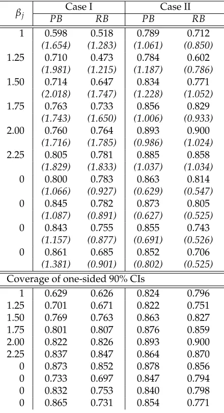
2.1 Empirical coverage of 90% confidence intervals for regression coeffi-cients over 1000 simulations under (n,p,p0) = (100, 10, 6) by Lasso

when the design is non-random. . . 75

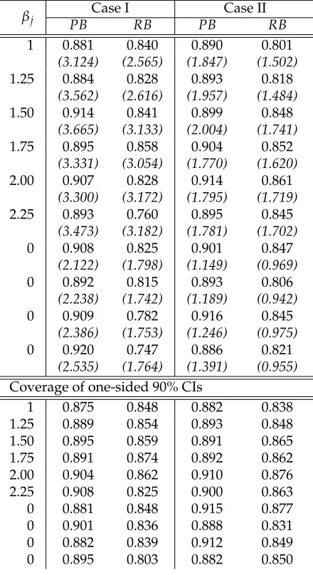
2.2 Empirical coverage of 90% confidence intervals for regression coeffi-cients over 1000 simulations under(n,p,p0) = (1000, 10, 6)by Lasso

when the design is non-random. . . 76

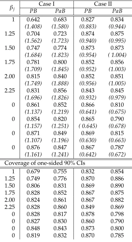
2.3 Empirical coverage of 90% confidence intervals for regression coeffi-cients over 1000 simulations under (n,p,p0) = (100, 10, 6) by Lasso

when the design is random. . . 77

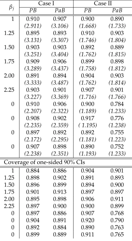
2.4 Empirical coverage of 90% confidence intervals for regression coeffi-cients over 1000 simulations under(n,p,p0) = (1000, 10, 6)by Lasso

when the design is random. . . 78

(15)

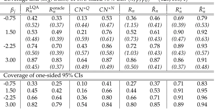
3.1 Empirical coverage of 95% confidence intervals for nonzero regression coefficients by Alasso under (n,p,p0) = (120, 100, 4) using ˜λn = 0 and crossvalidation choice ofλn. The medianλn choice was 0.79·n1/4. One-sided intervals are bounded in the sgn(βj)direction. . . 130 3.2 Empirical coverage of 95% confidence intervals for nonzero regression

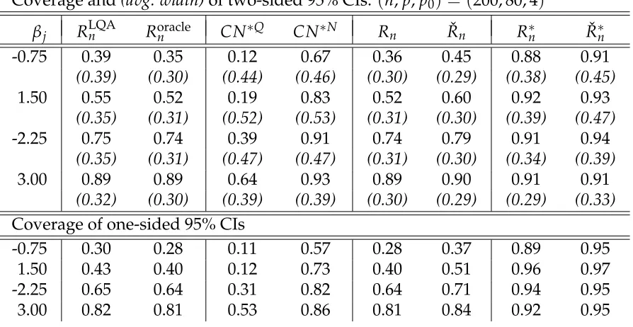
coefficients by Alasso under(n,p,p0) = (200, 80, 4)using ˜λn =0 and crossvalidation choice of λn. The median λn choice was 1.40·n1/4. One-sided intervals are bounded in the sgn(βj)direction. . . 131 3.3 Empirical coverage of 95% confidence intervals for nonzero regression

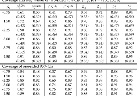
coefficients by Alasso under(n,p,p0) = (150, 250, 6)using

crossvalida-tion choices of ˜λn andλn. The median ˜λn andλnchoices were 0.01·n1/2 and 0.32·n1/4. One-sided intervals are bounded in the sgn(βj)direction.132 3.4 Empirical coverage of 95% confidence intervals for nonzero regression

coefficients by Alasso under(n,p,p0) = (150, 500, 8)using

(16)

List of Figures

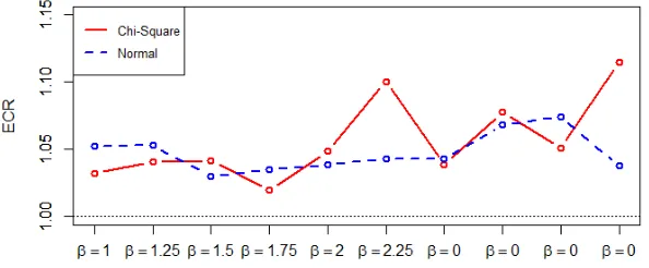
2.1 Ratio of Empirical Coverage of 90% CIs constructed by Perturbation and Residual Bootstrap in Lasso for Regression Coefficients . . . 79

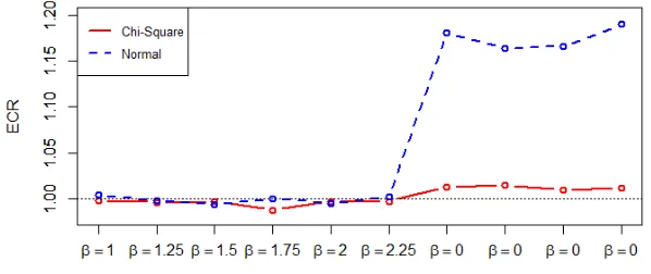
2.2 Ratio of Empirical Coverage of 90% CIs constructed by Perturbation and Paired Bootstrap in Lasso for Regression Coefficients . . . 80

3.1 Confidence intervals based onRLQAn (straight), ˇRn(wavy),CN∗N(jagged), and ˇR∗_n(wiggly) for each of the Alasso selected genes from theriboflavin

(17)

Chapter 1 Perturbation Bootstrap in Regression

M-estimation

1.1 Introduction

Consider the multiple linear regression model :

yi = x′iβ+ϵi, i =1, 2, . . . ,n (1.1.1) wherey1, . . . ,yn are responses,ϵ1, . . . ,ϵn are independent and identically distributed (iid) random variables with common distribution F(say),x1, . . . ,xn are known non random design vectors andβis the p-dimensional vector of parameters.

Supposeβ¯_n is the M-estimator ofβcorresponding to the objective functionΛ(·)i.e. ¯

βn =arg min_t∑n_i=1Λ(yi−x′it). Now ifψ(·)is the derivative of Λ(·), thenβn¯ is the M-estimator corresponding to the score functionψ(·)and is defined as the solution of the vector equation

n

∑

i=1

(18)

It is known [cf. Huber(1981)] that under some conditions on the objective func-tion, design vectors and error distribution F; (βn¯ −β) with proper scaling has an asymptotically normal distribution with mean0and dispersion matrix σ2Ip where σ2 =Eψ2(ϵ1)/E2ψ′(ϵ1).

After introduction of bootstrap by Efron in 1979 as a resampling technique, it has been widely used as a distributional approximation method. Resampling from the naive empirical distribution of the centered residuals in a regression setup, called residual bootstrap, was introduced by Freedman (1981). Freedman (1981) and Bickel and Freedman (1981b) had shown that given data, the conditional distribution of √

n(β∗_n−β¯n)converges to the same normal distribution as the distribution of √

n(β¯n− β)whenβ¯nis the usual least square estimator ofβ, that is, whenΛ(x) = x2. It implies that the residual bootstrap approximation to the exact distribution of the least square estimator is first order correct as in the case of normal approximation. The advantage of the residual bootstrap approximation over normal approximation for the distribution of linear contrasts of least square estimator for generalpwas first shown by Navidi (1989) by investigating the underlying Edgeworth Expansion (EE); although heuristics behind the same was given by Liu (1988) in restricted casep =1. Consequently, EE for the general M-estimator ofβwas obtained by Lahiri (1989b) whenp =1; whereas the same for the multivariate least square estimator was found by Qumsiyeh (1990a). EE of standardized and studentized versions of the general M-estimator in multiple linear regression setup was first obtained by Lahiri (1992). Lahiri (1992) also established the second order results for residual bootstrap in regression M-estimation.

(19)

sample from a weighted empirical distribution to obtain the bootstrap sample residu-als. Broadly, the resulting bootstrap procedure is called the weighted or generalized bootstrap. It was introduced by Mason and Newton (1992) for bootstrapping mean of a collection of iid random variables. Mason and Newton (1992) considered ex-changeable weights and established its consistency. Lahiri (1992) established second order correctness of generalized bootstrap in approximating the distribution of the M-estimator for the model (1.1.1) when the weights are chosen in a particular fashion depending on the design vectors. Wellner and Zhan (1996) proved the consistency of infinite dimensional generalized bootstrapped M-estimators. Consequently, Chatterjee and Bose (2005) established distributional consistency of generalized bootstrap in estimating equations and showed that generalized bootstrap can be used in order to estimate the asymptotic variance of the original estimator. Chatterjee and Bose (2005) also mentioned the bias correction essential for achieving second order correctness. An important special case of generalized bootstrap is the bayesian bootstrap of Rubin (1981). Rao and Zhao (1992) showed that the distribution function of M-estimator for the model (1.1.1) can be approximated consistently by bayesian bootstrap. See the monograph of Barbe and Bertail (2012) for an extensive study of generalized bootstrap.

(20)

distribution of the least square estimator upto second order in heteroscedastic setup and described a modification in resampling procedure which can establish second order correctness. For generalp, the heuristics behind achieving second order correct-ness by wild bootstrap in homoscedastic least square regression were discussed in Mammen (1993). Recently, Kline and Santos (2011) developed a score based bootstrap method depending on wild bootstrap in M-estimation for the homoscedastic model (1.1.1) and established consistency of the procedure for Wald and Lagrange Multiplier type tests for a class of M-estimators under misspecification and clustering of data.

(21)

bootstrap method can also be used in regression M-estimation for making inferences regarding the regression parameters and higher order accuracy can be achieved than the normal approximation.

A classical way of studentization in bootstrap setup, in case of regression M-estimator and for iid errors, is to consider the studentization factor to beσn∗ =s∗nτn∗−1, τn∗ = n−1∑in=1ψ′(ϵ∗i), s∗n2 = n−1∑in=1ψ2(ϵ∗i) where ϵi∗ = yi−x′iβ∗n, i ∈ {1, . . . ,n}, with β∗_n being the perturbation bootstrapped estimator of β, defined in Section 1.2. Although the residual bootstrapped estimator is S.O.C. after straight-forward studen-tization, the same pivot fails to be S.O.C. in the case of perturbation bootstrap. Two important special cases are considered as examples in this respect. The reason behind this failure is that although the bootstrap residuals are sufficient in capturing the vari-ability of the bootstrapped estimator in residual bootstrap, it is not enough in the case of perturbation resampling. Modifications have been proposed as remedies and are shown to be S.O.C. The modifications are based on the novel idea that the variability of the random perturbing quantitiesG∗_i (1≤i ≤n) along with the bootstrap residuals are required to capture the variability of the perturbation bootstrapped estimator; whereas individually they are not sufficient. For technical details, see Section1.4.3and Section1.5.1.

(22)

finding EE have been demonstrated and discussed in Bhattacharya and Ghosh (1978), Bhattacharya and Rao (1986), Navidi (1989) and Lahiri (1992).

A significant volume of chapter is available in bootstrapping M-estimators. We will conclude this section by briefly reviewing the literature. bootstrapping M-estimators in linear model has been studied by Navidi(1989), Lahiri (1992, 1996), Rao and Zhao (1992), Qumsiyeh (1994), Karabulut and Lahiri (1997), Jin, Ying and Wei (2001), Hu (2001), El Bantli (2004) among others. And in the applications other than linear model, bootstrapping in M-estimation and its subclasses has been investigated by Arcones and Giné (1992), Lahiri (1994), Wellner and Zhan (1996), Allen and Datta (1999), Hu and Kalbfleisch (2000), Hlavka (2003), Wang and Zhou (2004), Chatterjee and Bose (2005), Ma and Kosorok (2005), Lahiri and Zhu (2006), Cheng and Huang (2010), Feng et. al. (2011), Lee (2012), Cheng (2015), among others.

The rest of the chapter is organized as follows. Perturbation bootstrap is described briefly in Section 1.2. Section 1.3 states the assumptions and motivations behind considering those assumptions. Main results for iid case, along with the modification in bootstrap studentization, are stated in Section 1.4. An extension to the case of independent and non-iid errors is proposed in Section1.5. Proofs are given in Section

1.6. Section1.7states concluding remarks.

1.2 Description of Perturbation Bootstrap

(23)

bootstrap. More precisely, the perturbation bootstrap estimatorβ∗_n is defined as

β∗_n =arg min t

n

∑

i=1

Λ(yi−x′it)G ∗ i

or in terms of the score functionψ(·), as the solution of the vector equation n

∑

i=1

xiψ(yi−x′iβ)Gi∗ =0 (1.2.1)

where G∗_i,i ∈ {1, . . . ,n} are non-negative and non-degenerate completely known random variables, considered as perturbation quantities. Note that, ifµG∗ is the mean ofG₁∗, thenβn¯ is the solution ofE

(

∑n

i=1xiψ(ϵ¯i)Gi∗|ϵ1, . . . ,ϵn

)

=∑n_i₌₁xiψ(ϵ¯i)µG∗ =0 where ¯ϵi =yi−xi′β¯n,i∈ {1, . . . ,n}, are the residuals corresponding to the M-estimator

¯

β_n. This observation will be helpful in finding a suitable stochastic approximation in bootstrap regime. For details, see Section1.6.

The central idea of the perturbation bootstrap is to draw a relatively large collection of iid random samples {(G₁∗b, . . . ,G∗_nb) : b = 1, . . . ,B} from the distribution of G₁∗

and then to find the conditional empirical distribution of√n(β∗_n −β¯n) given data

yi : i=1, . . . ,n, by solving n

∑

i=1

xiψ(yi−x′iβ)G ∗b i =0

for eachb∈ {1, . . . ,B}; to approximate the distribution of√n(βn¯ −β)asymptotically. As a result the bootstrapped distribution may be used as an approximation to the original distribution, just like the normal approximation, in constructing confidence intervals and testing of hypotheses regardingβ.

(24)

the least square setup i.e. Λ(x) = x2. In this caseβ∗_n takes the form

β∗_n =

( n

∑

i=1

xix′_iG∗i

)−1( n

∑

i=1

xiyiGi∗

)

(1.2.2)

indicating that the perturbing quantitiesG∗_i’s can be thought of as weights.

Remark 1.2.1 Consider the least square estimatorβˆn. Then keeping the asymptotic properties

fixed, the perturbation bootstrap versionβˆ∗_1n ofβnˆ can be defined alternatively as the solution

of

n

∑

i=1

xi(yi−x′iβ)

(

G_i∗−µG∗

)

+

n

∑

i=1

xix′_i(βnˆ −β)(2µG∗ −Gi∗

)

=0

which in turn implies thatβˆ∗_1nis the solution of n

∑

i=1

xi(z∗i −x′iβ) =0 (1.2.3)

where z∗_i =x′_iβnˆ +ϵˆi[µ−_G∗1(G_i∗−µG∗)],ϵˆi =yi−x′iβnˆ , i ∈ {1, . . . ,n}. On the other hand,

the simple wild bootstrap versionβˆ∗_2n ofβnˆ is defined as the solution of n

∑

i=1

xi(y∗i −x′iβ) =0 (1.2.4)

where y∗_i = x′_iβnˆ +ϵˆiti, i ∈ {1, . . . ,n}. {t1, . . . ,tn} is a set of iid random variables

inde-pendent of {ϵ1, . . . ,ϵn} with Et1 = 0, Var(t1) = 1. Additionally, one needs E(t31) = 1 for establishing second order correctness of wild bootstrap approximation [cf. Liu (1988),

Mammen (1993)]. Now Looking at (1.2.3) and (1.2.4) and in view of assumption (A.5)(ii), it

can be said that the perturbation bootstrap coincides with the wild bootstrap in least square

setup. Therefore one can view perturbation bootstrap as a generalization of the wild bootstrap

(25)

Remark 1.2.2 There is a basic difference between perturbation bootstrap and weighted boot-strap with respect to the construction of the bootboot-strapped estimator. Whereas in the perturbation

bootstrap, the bootstrapped estimator is defined through the non-negative and non-degenerate

random perturbations of the objective function; in weighted bootstrap, the bootstrapped

estima-tor is defined through bootstrap samples drawn from a weighted empirical distribution. See for

example the construction of the weighted bootstrapped estimator corresponding to Theorem 2.3

of Lahiri (1992) and compare it with our construction as stated in Section1.2. However, one

can think the perturbation bootstrap defined in Section1.2as the weighted bootstrap version of

some statistical functional if the design vectors are random. Suppose,{(x1,y1). . . ,(xn,yn)}

are iid with underlying probability measureQ. Then one can think

β=T(Q) = arg min t

E[Λ(yi−x′it)

]

for some statistical functional T(·). Define the empirical measuresQn =n−1∑ni=11(xi,yi)

and Qn,G∗ = n−1∑n_i₌₁1(x_i,y_i)G∗

i where 1(·) is the indicator function. Then we have ¯

β_n = T(Qn) and β∗_n = T(Qn,G∗). This is the general setup of Barbe and Bertail (2012).

Second order results are available only in standardized setup for differentiable statistical

functionals, see Section 3.1 of Barbe and Bertail (2012). In particular, second order correctness

of weighted bootstrap of standardized mean of iid random variables was established by Haeusler

et. al. (1991). On the other hand, we have assumed the design vectors to be non-random,

implying that our setup does not quite fit in the general statistical functional setup of Barbe

and Bertail (2012); although Theorem1.4.3continue to hold when the design is random. Our

main motivation is to explore second order results in studentized setup which is the common

setup in practice. We have also extended second order correctness of perturbation bootstrap

(26)

chapter significantly extends the results available in the literature of second order correctness

by bootstrap in regression M-estimation.

1.3 Assumptions

Suppose,xi = (xi1,xi2, . . . ,xip)′. Define,Dn ≡D= (∑n_i=1xix′i)1/2, An =n−1D2,di = D−1xi, 1≤i ≤nandq = p(p+1)

2 . Also define,q×1 vectorzi = (x

2

i1,xi1xi2, . . . ,xi1xip

,x2_i₂,xi2xi3, . . . ,xi2xip, . . . ,xip2)′. Note that for any constantsai, . . . ,an ∈ R,∑n_i=1aizi = 0which implies and is implied by∑n_i₌₁aixix′_i = 0. Hence,{z1, . . . ,zn} are linearly independent if and only if{xix_i′: 1 ≤i ≤n}are linearly independent. Therefore,rn = the rank of∑n_i=1ziz′_i is nondecreasing in n. So, if r =max{rn : n≥ 1}then without loss of generality (w.l.g.), we can assume thatrn =rfor alln≥q. Consider canonical decomposition of∑_in=1ziz′i as

L(

n

∑

i=1

ziz′_i)L′ =

[

Ir 0 0 0

]

where Lis a q×q non-singular matrix. Partition Las L′ = [L₁′ L′₂], where L1 is of orderr×q. Definer×1 vectorz˜i by

˜

zi =L1zi, 1 ≤i ≤n

Note that ∑_in₌₁z˜iz˜′_i = L1(∑n_i=1ziz′i)L′1 = Ir. Suppose, vi = (x′iψ(ϵ1),z′iψ′(ϵ1))′. ˘

zi = (z′_i,n−1)′.

(27)

h that is twice differentiable. Also ||.|| denotes euclidean norm.For any set B ∈ Rp _and

ϵ > 0, δB denotes the boundary of B, |B| denotes the cardinality of B and

Bϵ ₌ _{x _: _x _∈ Rp _and _d(_x_,_B) _<

ϵ} where d(x,B) = inf{||x−y|| : y ∈ B}. For a function f : Rl → R and a non-negative integral vector α = (α1,α2, . . . ,αl)′,

Dα_f ₌_Dα1

1 . . .D αl

l f, whereD αj

j f denotesαjtimes partial derivative of f with respect to the jth component of its argument, 1 ≤ j ≤ l. Also assume that (e1, . . . ,ep)′ is the standard basis ofRp. Let,P∗ andE∗ respectively denote conditional bootstrap probability and conditional expectation ofG₁∗given data. The class of setsB denotes the collection of borel subsets ofRp satisfying

sup B∈B Φ

((δB)ϵ) =O(ϵ) as ϵ ↓0 (1.3.1)

Next we state the assumptions:

(A.1) ψ(·)is twice differentiable andψ′′(·)satisfies a Lipschitz condition of orderαfor some 0 <2α ≤1.

(A.2) (i) An → A1asn→∞for some positive definite matrix A1.

(ii) E(n−1∑n_i₌₁viv′_i) → A2asn→∞for some non-singular matrix A2, where expectation is with respect to F.

(ii)′ E(n−1∑n_i=1v˜iv˜_i′) → A3 asn→ ∞for some non-singular matrix A3where ˜

vi is defined as same way asvi withzi being replaced byz˘i. (iii) nα/2₍∑n

i=1||di||6+2α)1/2+∑ni=1||z˜i||4=O(n−1)

(A.3) (i) Eψ(ϵ1) =0 andσ2 =Eψ2(ϵ1)/E(ψ′(ϵ1)) ∈ (0,∞).

(28)

(A.4) G∗_i andϵi are independent for all 1≤i≤n. (A.5) (i) EG∗₁3<∞

(ii) Var(G₁∗) = µ2_G∗,E(G₁∗−µG∗)3 =_µ3

G∗.

(iii) (

G₁∗−µG∗

)

satisfies Cramer’s condition: lim sup_|_t_|→_∞⏐⏐E

(

exp(

it(

G₁∗−µG∗)))⏐⏐<1.

(iii)′((G₁∗−µG∗),(G∗

1 −µG∗

)2)

satisfies Cramer’s condition: lim sup_||₍_t₁_,_t₂₎_||→_∞

⏐ ⏐ ⏐E

(

exp(it1

(

G₁∗−µG∗)+it₂(G∗

1−µG∗

)2))⏐ ⏐ ⏐<1

(A.6) (i) (ψ(ϵ1),ψ′(ϵ1)

)

satisfies Cramer’s condition: lim sup_||₍_t

1,t2)||→∞

⏐ ⏐ ⏐E

(

exp(

it1ψ(ϵ1) +it2ψ′(ϵ1)

))⏐ ⏐ ⏐ <1

(i)′(

ψ(ϵ1),ψ′(ϵ1),ψ2(ϵ1)

)

satisfies Cramer’s condition: lim sup_||₍_t

1,t2,t3)||→∞

⏐ ⏐ ⏐E

(

exp(

it1ψ(ϵ1) +it2ψ′(ϵ1) +it3ψ2(ϵ1)

))⏐_⏐

⏐<1

Definev¯i = (x¯′i,z¯′_i)′ where x¯i = xiψ(ϵ¯i),z¯i =ziψ′(ϵ¯i);{ϵ¯1, . . . , ¯ϵn}being the set of residuals. Also, define A¯2n = n−1∑n_i=1x¯ix¯′i and A¯1n = n−1∑in=1xix′iψ′(ϵ¯i). Note thatn−1∑n_i=1v¯iv¯′i is an estimate of the matrixE(n−1∑ni=1vivi′)and due to assumption (A.2)(ii), ∑n_i=1v¯iv¯i′ is non-singular for sufficiently large n. Hence, without loss of generality the canonical decomposition of_∑n_i₌₁v¯iv¯′_i can be assumed as

B( n

∑

i=1

¯ viv¯_i′

)

B′ =Ik

wherek= p+qandBis ak×knon-singular matrix. Definek×1 vectorv˘i by

˘

vi = Bv¯i, 1 ≤i ≤n

(29)

Navidi (1989)] is also required:

(A.7) There exists aδ >0 such that−Kn(δ)/logγn →∞where Bn(δ) ={1≤i ≤n:

(v˘_i′t)2 >δγ2n for allt ∈Rkwith||t||2 =1},Kn(δ) =|Bn(δ)|, the cardinality of the set Bn(δ), andγn = (∑_in=1||v˘i||4)1/2.

But note that the condition (A.7) has already been satisfied in our set up due to Lemma1.6.4and the proposition in Lahiri (1992).

Now we briefly explain the assumptions. Assumption (A.1) is smoothness con-dition on the score functionψ(·). This condition is essential for obtaining a Taylor’s expansion ofψ(·)around regression errors. Assumption (A.2) presents the regularity conditions on the design vectors necessary to find EE. For the validity of asymptotic normality of the regression M-estimator, only (A.2)(i) is enough [cf. Huber (1981)]; whereas additional condition (A.2)(ii) is required for the validity of the EE. (A.2)(iii) states atmost how fast theL2norm of the design vectors can increase to get a valid EE. This condition is somewhat stronger than the condition (C.6) assumed in Lahiri (1992); although there was a reduction in accuracy of bootstrap approximation due to this relaxation. This type of conditions are quite common in the literature of edgeworth expansions in regression setup; see for example Navidi (1989), Qumsiyeh (1990a). We now state an example where assumption (A.2) (iii) is fulfilled.

Example 1.3.1 Suppose, {X(1)_{, . . . ,}_X(p)_} _{is a set of independent random vectors where} X(j) = (X1j, . . . ,Xnj)′is a vector of n iid copies of the non-degenerate random variable X1j,

j ∈ {1, . . . ,p}. Define, p×p matrix M = ((mjk))j,k=1,...,p where mjk = E(X12jX21k) and

n×p matrix X =(

X(1), . . . ,X(p))

(30)

all j ∈ {1, . . . ,p} anddet(M) ̸= 0. Then for the design matrix X, assumption (A.2) (iii)

holds with probability 1 (w.p. 1).

proof :

For the design matrixX,xi = (Xi1,Xi2, . . . ,Xip)′andzi = (X2_i₁,Xi1Xi2, . . . ,Xi1Xip,X2i2

,Xi2Xi3, . . . ,Xi2Xip, . . . ,X_ip2)′fori ∈ {1, . . . ,n}.

First note that if all the entries of X are iid then the condition det(M) ̸= 0 is redundant. By Kolmogorov strong law of large numbers, An = n−1D2 → diag( E(X₁₁2 ), . . . ,E(X2₁_p))

andn−1∑n_i=1||xi||6+2α →E||x1||6+2αbothw.p.1 and hence

nα/2( n

∑

i=1

||di||6+2α

)1/2

≤nα/2_||D−1_||3+α( n

∑

i=1

||xi||6+2α

)1/2

=O(n−1) w.p.1 (1.3.2)

Again, sinceMis a non-singular matrix,n−1_∑_in₌₁ziz′_i → N w.p.1, for some positive definite matrixN. This implies that||L||=O(n−1/2) w.p.1 and hence

n

∑

i=1

||z˜i||4 ≤ ||L||4 n

∑

i=1

||zi||4

=O(n−1) w.p.1 (1.3.3)

Therefore, our claim follows from (1.3.2) and (1.3.3).

(31)

smoothness conditions on the perturbing quantitiesG∗_i’s, required for the valid two term EE in bootstrap setup. The Cramer’s condition is very common in the literature of edgeworth expansions. Cramer’s condition is satisfied when the distribution of(G₁∗− µG∗)or((G1∗−µ∗G),(G∗1−EG1∗)2)has a non-degenerate component which is absolutely

continuous with respect to Lebesgue measure [cf. Hall (1992)]. An immediate choice of the distribution ofG₁∗is Beta(γ,δ) where 3γ =δ =3/2. Also one can investigate

Generalized Beta family of distributions for more choices of the distribution of G₁∗. Assumption (A.6) is the Cramer’s condition on the errors. Although this assumption is not needed for obtaining EE of the bootstrapped estimators, it is needed for obtaining EE for the original M-estimator.

Note that the condition (A.7) is somewhat abstract. Hence as pointed out by a referee, some clarification would be helpful. To this end, it is worth mentioning that to find formal EE for the standardized bootstrapped pivot (see section1.4.1), the most difficult step is to show

max |α|≤p+q+4

∫

C1≤γn||t||≤C2

|DαE∗eit′T

∗

n_|_d_t ₌_o

p(n−1/2) (1.3.4) whereC1,C2are non-negative constants andT∗n = ∑ni=1

( _˘

X_i∗−E∗(X˘_i∗)), withX˘_i∗ =

˘

vi(Gi−µG∗)1(||v˘_i(G_i−_µ_G∗)|| ≤1). Now it is easy to see that for any|_α| ≤ p+q+4,

|Dα_E∗_eit′T∗_n_|_{is bounded above by a sum of}_n|α|_{-terms, each of which is bounded above} by

C(α)·max{E∗||X˘_i∗−E∗(X˘_i∗)|||α| : i∈ I_n∗} ·

∏

i∈_I_n∗c

|E∗eit′X˘i∗_|

(32)

Now note that for alli ∈ {1, . . . ,n},

E∗||_X˘∗

i −E∗(X˘i∗)|| |α| _≤

2|α|

and |E∗eit′X˘i∗_{| ≤ |}_E∗_eit

′

˘

vi(Gi−µ_G∗)_|₊

2P∗(

||v˘i(Gi−µG∗)|| >1)

Hence, in view of Cramer’s condition (A.5) (iii) and Lemma1.6.4, if there exists a sequence of sets{Jn}n≥1such that Jn ⊂ {1, . . . ,n}and for alli∈ Jn,γ−_n1|t′v˘i|>ξ for someξ >0, then for some 0 <θ <1 we have

sup{

∏

i∈I_n∗c

|E∗eit′X˘i∗_| _: _C₁_≤_γ_n_{||t|| ≤}_C₂}

≤sup{

∏

i∈I_n∗c∩J_n

|E∗eiγn−1t

′ _˘

X_i∗_|_: _C

1 ≤ ||t|| ≤C2

}

≤θ|I ∗c

n ∩Jn| _(1.3.5)

Again,|I_n∗c∩ Jn| ≥ |Jn| − |α|andγn ≥kn−1. Therefore, to achieve (1.3.4), it is enough to have

n2(p+q)+4·θ|Jn|−(p+q+4) =o(n−1/2)

Hence due to Lemma1.6.4, it is enough to have|Jn| ≥ an−C·logγn for some positive constantCand a sequence of constants{an}increasing to∞. This observation together with (1.3.5) justifies condition (A.7).

(33)

1.4 Main Results

1.4.1 Rate of Perturbation Bootstrap Approximation

Here we will state the approximation results both in standardized and studentized setup. It is well known that√nβn¯ has asymptotic varianceσ2A−n 1. So, the standard-ized version of the M-estimatorβn¯ is defined asFn =

√

nσ−1A1/2_n (βn¯ −β). Now to define the standardized version of the corresponding bootstrapped statistic β∗_n, we need its conditional asymptotic variance, given the data. Using Taylor’s expansion, it is quite easy to get the conditional asymptotic variance of√nβ∗_n as A¯_1n−1A¯2nA¯_1n−1. Note that inverse of the matricesA¯_1n−1andA¯−_2n1are well defined for sufficiently large sample size n due to the assumption (A.2)(i) and (A.3)(ii). Hence, the standardized bootstrapped M-estimatorF_n∗ can be defined as

Fn∗ = √

nΣ¯−n 1/2(β∗_n−β¯n)

whereΣ¯−n 1/2 = A¯2n−1/2A¯1n,A¯1/22n being defined in terms of the spectral decomposition ofA¯2n; although it can be defined in many different ways [cf. Lahiri (1994)]. Under some regularity conditions, both the distribution ofFnand the conditional distribution of F_n∗ can be shown to be approximated asymptotically by a Normal distribution with mean0and varianceIp. Hence, it is straightforward that perturbation bootstrap approximation to the distribution of the M-estimator is first order correct. The second order result in standardized case is formally stated in Theorem1.4.1.

(34)

statistics{β∗_n}n≥1such that

P∗(

β∗_n solves (1.2.1) and||β∗_n −βn¯ || ≤C1.n−1/2.(logn)1/2

)

≥1−δnn−1/2

whereδn ≡δn(ϵ1, . . . ,ϵn)tends to 0.

Theorem 1.4.1 Let{β∗_n}n≥1be a sequence of statistics satisfying Proposition1.4.1depending on(ϵ1, . . . ,ϵn). Assume, the assumptions(A.1)-(A.5)hold.

(a) Then there exist constant C2>0and a sequence of Borel setsQ2n ⊆Rnand polynomial

a∗n(·,ψ,G∗)depending on first three moments of G1∗and onψ(·),ψ′(·)&ψ′′(·)through the residuals{ϵ¯1, . . . , ¯ϵn}such that given(ϵ1, . . . ,ϵn) ∈ Q2n, withP((ϵ1, . . . ,ϵn) ∈ Q2n)→1, we have for n ≥C2,

sup B∈B

|P∗(F_n∗ ∈ B)−

∫

Bξ ∗

n(x)dx| ≤δnn−1/2

whereξ∗n(x) = (1+n−1/2a∗n(x,ψ,G∗))ϕ(x)andδn ≡δn(ϵ1, . . . ,ϵn)tends to 0.

(b) Suppose in addition assumption(A.6)(i)holds. Then we have,

sup B∈B ⏐

⏐P∗(F_n∗ ∈ B)−P(F_n ∈ B) ⏐

⏐=o_p(n−1/2)

Now, the quantityσ2is mostly unavailable in practical circumstances. Hence, the non-pivotal quantity like Fn is very rare in use in providing valid inferences. It is more reasonable to explore the asymptotic properties of a pivotal quantity, like the studentized version of the M-estimator β¯n. Depending on the observed residuals

¯

ϵi = yi−xi′β¯n, i ∈ {1, . . . ,n}, the natural way to define an estimator of σ2 is ˆσn2 where ˆσn =snτn−1,τn =n−1∑ni=1ψ′(ϵ¯i)ands2n =n−1∑ni=1ψ2(ϵ¯i). Hence, the studen-tized M-estimator in regression setup may be defined as Hn =

√

(35)

Similarly, studentized version of the corresponding bootstrapped estimator can be construed as√nΣ¯∗−n 1/2(β∗_n −βn¯ )where Σ¯∗−n 1/2 is defined in the same way asΣ¯−n 1/2 after replacing ¯ϵi by ϵ∗_i, ϵ∗_i = yi−x′iβ∗n, for each i ∈ {1, . . . ,n}. But this definition requires to obtainΣ¯∗−n 1/2at each bootstrap sample(G₁∗b, . . . ,Gn∗b),b =1, . . . ,B. This is not computationally feasible since computation ofΣ¯∗−n 1/2involves matrix inversion. So, let us define the studentized bootstrapped M-estimator in more computationally feasible way as

H_n∗ =√nσn∗−1σˆnΣ¯−n 1/2(β∗_n −βn¯ )

whereσn∗ =s∗nτn∗−1,τn∗ =n−1∑ni=1ψ′(ϵi∗),s∗n2 =n−1∑ni=1ψ2(ϵi∗)and ˆσn2andΣ¯−n1/2are as defined earlier.

Theorem 1.4.2 Suppose, the assumptions(A.1)-(A.5)hold.

(a) Then there exist constant C3>0and a sequence of Borel setsQ3n ⊆Rnand polynomial ˜

a∗_n(·,ψ,G∗)depending on first three moments of G₁∗and onψ(·),ψ′(·)&ψ′′(·)through

the residuals{ϵ¯1, . . . , ¯ϵn}, such that given(ϵ1, . . . ,ϵn) ∈ Q3n, withP((ϵ1, . . . ,ϵn) ∈ Q3n)→1, we have for n ≥C3,

sup B∈B

|P∗(Hn∗ ∈ B)−

∫

B ˜

ξ∗_n(x)dx| ≤ δnn−1/2

whereξ˜∗n(x) = (1+n−1/2a˜∗n(x,ψ,G∗))ϕ(x)andδn ≡δn(ϵ1, . . . ,ϵn)tends to 0.

Suppose in addition assumption(A.6)(i)′ holds. Then

(b) for the collection of Borel setsBdefined by (1.3.1),

sup B∈B ⏐

⏐P∗(H_n∗ ∈ B)−P(H_n ∈ B) ⏐

(36)

(c) if 2Eψ2(ϵ1)Eψ(ϵ1)ψ′(ϵ1) ̸=Eψ′(ϵ1)Eψ3(ϵ1), then there existsϵ>0such that,

P(lim inf n→∞

√

n[sup B∈B ⏐

⏐P∗(H_n∗ ∈ B)−P(H_n ∈ B) ⏐ ⏐ ]

>ϵ

)

=1

Remark 1.4.1 Proposition 1.4.1 states that there exists a sequence of perturbation boot-strapped estimatorβ∗_n within a neighborhood of length C.n−1/2(logn)1/2 around the original

M-estimator β¯n outside a set of bootstrap probability op(n−1/2). This existence result is

essential in finding valid EEs in bootstrap regime. This can be compared with Theorem 2.3 (a)

of Lahiri (1992), where similar kind of result was shown in case of residual and generalized

bootstrap.

Remark 1.4.2 Note that, where as the error term in approximating the distribution of M-estimator by perturbation bootstrap is of order Op(n−1/2)in the prevalent studentize setup,

it reduces the order of the error of approximation to op(n−1/2)in simple standardized setup.

This means that the difference between coefficients corresponding to the term n−1/2in the EEs

of original and bootstrapped estimator can be made arbitrarily small in standardized setup, but

not in usual studentized setup.

Remark 1.4.3 To understand part (c) of Theorem1.4.2, consider the usual least square esti-mator. In least square setup, the condition in the Theorem1.4.2(c) reduces to Eϵ3 ̸=0. This

simply means that if the studentization in perturbation bootstrapped version is performed

analogously as in case of original least square estimator, then the bootstrap distribution can

not correct the original distribution upto second order. If this is investigated more deeply, then

it can be observed that the usual studentized perturbation bootstrap approximation can not

(37)

1.4.2 Examples

Theorem1.4.2concludes that the standard way of performing studentization of the bootstrapped estimator is first order correct. In order to show that the usual studen-tized setup is not second order correct, we consider following two important special cases withψ(x) = x.

Example 1.4.2.1

Consider the observations {y1, . . . ,yn} are coming from the distribution F with a location shiftµ. This in terms of regression model becomes

yi =µ+ϵi

Hence, in this setupp =1, β=µandxi =1 for alli ∈ {1, . . . ,n}.

It can be shown that in this setup, ˜ξn(·)and ˜ξ∗n(·), the EE ofHn andHn∗respectively, turn out to be

˜

ξn(x) =

[

1−n−1/2{˜

b11 d dx +6

−1_b_˜ 31 d

3

dx3

}]

ϕ(x) ˜

ξ∗_n(x) =

[

1−n−1/2{_˜

b₁₁∗ d dx +6

−1_b_˜∗

31 d3 dx3

}]

ϕ(x) where

˜

b11 =−2−1σ−3Eϵ₁3, ˜b31 =−2σ−3Eϵ3₁ ˜

b₁₁∗ =−2σn−1n−1∑ni=1ϵ¯i, ˜b₃₁∗ =σn−3−12σn−1n−1∑ni=1ϵ¯i.

It is clear that ˜b₁₁∗ as well as ˜b∗₃₁ are not converging respectively to ˜b11 and ˜b31 in

(38)

Example 1.4.2.2

Consider the simple linear regression model

yi =β0+β1xi+ϵi

where β0 and β1 are parameters of interest and ϵi’s are iid errors. This model, in terms of our multivariate linear regression structure, can be written asyi = x˜i′β+ϵi whereβ= (β0,β1)′ andx˜i = (1,xi)′. Hence, the EEs of the original and bootstrapped estimators upto the ordero(n−1/2), after usual studentization, respectively becomes

˜

ξn(y1,y2) =

[

1−n−1/2{ 2

∑

j=1

˜

b₁₁∗(j) ∂

∂yj

+ 3

∑

j=0

˜

b(₃₁j,3−j) j!(3−j)!D

(j,3−j)}

]

ϕ(y1,y2)

˜

ξ∗n(y1,y2) =

[

1−n−1/2{ 2

∑

j=1

˜

b₁₁∗(j) ∂

∂yj

+ 3

∑

j=0

˜

b₃₁∗(j,3−j) j!(3−j)!D

(j,3−j)}

]

ϕ(y1,y2)

where ˜

b₁₁(j) =−2−1[n−1_∑n_i₌₁e′_jA−1_n /2˜xi

]

γ1

˜

b(j1,j2)

31 =−2

[

n−1∑n_i=1(e′1A−1n /2˜xi)j1(e′2An−1/2˜xi)j2

]

γ1

˜

b₁₁∗(j) =op(1)

˜

b∗(j1,j2)

31 =

[

n−1∑n_i=1(e′1A¯ −1/2

2n ˜xi)j1(e′2A −1/2

2n ˜xi)j2ψ3(ϵ¯i)

]

+op(1)

where j = 1 or 2, j1,j2 ∈ {0, 1, 2, 3} such that j1+j2 = 3, γ1is the coefficient of

skewness ofϵ1,A¯2n is as defined in general setup andAn =n−1∑n_i=1˜xi˜x′i =

[

1 x¯ ¯

x x¯2

(39)

where ¯x =n−1∑n_i=1xi and ¯x2 =n−1∑ni=1x2i.

Therefore, it is clear that the naive studentized bootstrapped estimator does not correct for the skewness corresponding to the original version in simple linear regres-sion setup. The usual studentization in perturbation bootstrap becomes second order correct only ifEϵ3₁ =0.

Note that, the coefficients ˜b₁₁(j), 1≤ j≤ p, all can not vanish together unlessγ1 =0

and hence ˜b∗₁₁(j) can not converge to ˜b₁₁(j)unless γ1=0. Similarly, it can be shown that

same condition is required to have the closeness of the coefficients ˜b₃₁(j,3−j) and ˜b∗₃₁(j,3−j). Hence, the two EEs can not get closer unlessγ1 =0, similar to the Example 1.4.2.1.

This is exactly what is stated in the part (c) of Theorem1.4.2in most general form.

1.4.3 Modification to the bootstrapped pivot

As it has been seen that Hn∗, the usual studentized version of the perturbation boot-strapped estimator is not attending the desired optimal rate op(n−1/2), so in the perspective of statistical inference, perturbation bootstrap is not advantageous over asymptotic normal approximation. For the sake of obtaining second order correctness, define the modified studentizedβ∗_n as

˜

H_n∗ =√n(σ˜_n∗)−1σˆnΣ¯−n 1/2(β∗_n −β¯n) (1.4.1)

where ˜

σ_n∗ =s˜∗_nτ˜_n∗−1, ˜τ_n∗ =n−1∑n_i=1ψ′(ϵ∗i)Gi∗, ˜s∗n2 =n−1∑ni=1ψ2(ϵ∗i)(Gi∗−µG∗)2.

The bootstrapped statistic H˜_n∗can be seen to be achieving the optimal rate, namely

(40)

Theorem 1.4.3 Suppose, the assumptions(A.1)′-(A.5)′hold. Also assume EG₁∗4 <∞.

(a) Then there exist constant C4>0and a sequence of Borel setsQ4n ⊆Rnand polynomial ¯

a∗n(·,ψ,G∗)depending on first three moments of G1∗and onψ(·),ψ

′₍_·₎

&ψ′′(·)through

the residuals{ϵ¯1, . . . , ¯ϵn}, such that given(ϵ1, . . . ,ϵn) ∈ Q4n, withP((ϵ1, . . . ,ϵn) ∈ Q4n)→1, we have for n ≥C4,

sup B∈B

|P∗(H˜_n∗ ∈ B)− ∫

B ¯

ξ∗_n(x)dx| ≤ δnn−1/2

whereξ¯∗n(x) = (1+n−1/2a¯∗n(x,ψ,G∗))ϕ(x)andδn ≡δn(ϵ1, . . . ,ϵn)tends to 0. (b) Suppose, in addition (A.6)(i)′ holds. Then, for the collection of Borel sets defined by

(1.3.1),

sup B∈B ⏐

⏐P∗(H˜_n∗ ∈ B)−P(H_n ∈ B) ⏐

⏐=o_p(n−1/2)

Remark 1.4.4 The modification that is needed to make the perturbation bootstrap method correct upto second order, suggests that besides incorporating the effect of bootstrap

random-ization throughψ(·) and ψ′(·) in the studentization factor of the bootstrap estimator, it is

also essential to blend properly the effect of randomization that is coming directly from the

perturbing quantities G_i∗s.

Remark 1.4.5 As pointed out by a referee, the usefulness of the above results depend critically on the rate of the probability P((ϵ1, . . . ,ϵn ∈ Qin)

)

, i = 1, 2, 3, 4. Following the steps of the proofs, it can be shown that P((ϵ1, . . . ,ϵn ∈ Qn)) = 1−O(n−1/2(logn)−2+γ2)

whereQn =∩4_i=1Qin, for someγ2∈ (0, 2), although the rate can be improved under moment condition stronger than (A.3) (ii). In general, ifE|ψ(ϵ1)|2γ3+E|ψ′(ϵ1)|2γ3+E|ψ′′(ϵ1)|γ3 < ∞for some natural numberγ3 ≥2, then analogously it can be shown thatP((ϵ1, . . . ,ϵn ∈ Qn)

)

=1−O(n−(2γ3−3)/2₍_log_n)−γ3+γ2)_{for some}_γ

(41)

order correctness of perturbation bootstrap can be established in almost sure sense under higher

moment condition.

Remark 1.4.6 The condition (1.3.1) on the collection of Borel subsets B of Rp, that is considered in the above theorems, is somewhat abstract. This condition is needed for achieving

two goals. One is to obtain valid EE for the normalized part of the underlying pivot [cf.

Corollary 20.4 of Bhattacharya and Rao (1986)] and the other one is to bound the remainder

term with an order o(n−1/2)with probability (or bootstrap probability)1−o(n−1/2). These two together allow us to get EE for the underlying pivots. A natural choice forB is the

collection of all Borel measurable convex subsets ofRp.

1.5 Extension to independent and non-identically

dis-tributed errors

In this section, we will extend second order results of perturbation bootstrap to the model (1.1.1) with independent and non-identically distributed [hereafter referred to as non-iid] errors. Clearly the case of non-iid errors includes the situation when the regression errors are heteroscedastic. In many practical situations, the measurements obtained have different variability due to a number of reasons and hence it is crucial for an inference procedure to be robust towards the presence of heteroscedasticity. We will show that perturbation bootstrap can approximate the exact distribution of the regression M-estimatorβn¯ upto second order even when the errors are non-iid.

(42)

(A.2)(iii)′′n−2∑n_i=1||xi||12+∑ni=1

[

||z˜i||4max{1,E|ψ′(ϵi)|4}

]

=O(n−1). (A.3)(i)′′ Eψ(ϵi) = 0 for alli ∈ {1, . . . ,n}.

(A.3)(ii)′′ n−1_∑n_i₌₁[

E|ψ(ϵi)|6+υ+E|ψ′(ϵi)|6+υ+E|ψ′′(ϵi)|4+υ

]

=O(1) for someυ > 0.

(A.6)(i)′′ (ψ(ϵn),ψ′(ϵn),ψ2(ϵn))∞_n₌₁satisfies Cramer’s condition in a uniform sense i.e. for any positive b,

lim sup

n→∞ ||(t1,supt2,t3)||>b

⏐ ⏐ ⏐E

(

exp(

it1ψ(ϵn) +it2ψ′(ϵn) +it3ψ2(ϵn)))

⏐ ⏐ ⏐ <1.

(A.8) A1n and A2n both converge to non-singular matrices asn→∞.

We will denote the assumptions (A.1)-(A.4) by (A.1)′′-(A.4)′′when (A.2) is defined with (iii)′′ instead of (iii) and (A.3) is defined with (i)′′, (ii)′′ in place of (i) and (ii) respectively.

1.5.1 Rate of Perturbation Bootstrap Approximation

Note that when the regression errors are non-identically distributed,√nβn¯ has asymp-totic variance A−_1n1A2nA−_1n1. Hence, the natural way of defining studentized pivot corresponding toβn¯ is

˘ Hn =

√

nΣ¯−n 1/2(βn¯ −β)

whereΣ¯−n1/2 = A¯−_2n1/2A¯1n with A¯1n = n−1∑n_i=1xixi′ψ′(ϵ¯i),A¯2n = n−1∑n_i=1 xix′iψ2(ϵ¯i) and ¯ϵi =yi−xi′βn,¯ i ∈ {1, . . . ,n}. Define the corresponding bootstrap pivot as

˘ Hn∗ =

√

(43)

where Σ∗−n 1/2 = A∗−_2n 1/2A_1n∗ with ϵ∗_i = yi−x′iβn∗, A∗1n = n−1∑ni=1xix′iψ′(ϵ∗i)G ∗ i and A∗_2n =n−1_∑_in₌₁xix′_iψ2(ϵ∗_i)(Gi−µG∗)2,i ∈ {1, . . . ,n}.

Theorem 1.5.1 Suppose, the assumptions(A.1)′′-(A.4)′′and(A.5)(i)hold.

(a) Then there exist constant C5 > 0and a sequence of Borel sets Q5n ⊆ Rn, such that P((ϵ1, . . . ,ϵn) ∈ Q5n) → 1as n → ∞, and given(ϵ1, . . . ,ϵn) ∈ Q5n, n ≥C5such that there exists a sequence of statistics{β∗_n}n≥1such that

P∗(

β∗_n solves(1.2.1) and ||β∗_n−βn¯ || ≤C5.n−1/2.(logn)1/2

)

≥1−o(

n−1/2)

(b) Suppose in addition(A.5)(ii),(iii)′and(A.8)hold. Then there exist polynomiala˘∗_n(·,ψ,G∗)

depending on first three moments of G∗₁and onψ(·),ψ′(·)&ψ′′(·)through the residuals {ϵ¯1, . . . , ¯ϵn}, such that given(ϵ1, ...,ϵn) ∈ Q5n, we have for n ≥C5,

sup B∈B|P∗(

˘

H_n∗ ∈ B)− ∫

B ˘

ξ∗n(x)dx| ≤ δnn−1/2

whereξ˘∗_n(x) = (1+n−1/2a˘∗_n(x,ψ,G∗))ϕ(x)andδn ≡δn(ϵ1, . . . ,ϵn)tends to 0.

(c) Suppose, in addition to the assumptions (A.1)′′-(A.4)′′, (A.5)(i),(ii),(iii)′ and (A.8),

(A.6)(i)′′holds. Then, for the collection of Borel sets defined by (1.3.1),

sup B∈B ⏐

⏐P∗(H˘_n∗ ∈ B)−P(H˘_n ∈ B) ⏐

⏐=o_p(n−1/2)

Remark 1.5.1 The form of the studentized pivot H˘_n∗, defined for achieving second order correctness in non-iid case is different fromH˜_n∗, due to the difference in asymptotic variances ofβn¯ in two setups. In non-iid case, one cannot ignore computation of the negative square root

of a matrix at each bootstrap iteration. But Theorem1.5.1is more general than Theorem1.4.3

in the sense that it also includes the case when errors are iid. Note thatΣ¯∗n = A¯1n∗−1A¯∗2nA¯

(44)

where A¯∗_1n = n−1∑n_i=1xix′iψ′(ϵ∗i) and A¯

∗

2n = n−1∑ni=1xix′iψ2(ϵ∗i) and σ ∗

n = s∗nτn∗−1

whereτn∗ =n−1∑in=1ψ′(ϵi∗), s ∗2

n =n−1∑ni=1ψ2(ϵ∗i). We need to modifyΣ¯

∗

n and σn∗ toΣ∗n

andσ˜n∗respectively to achieve second order correctness.

Remark 1.5.2 There is no difference in employing perturbation bootstrap and the usual residual bootstrap with respect to the accuracy of inference. Under some mild conditions, both

are second order correct. But in view Theorem1.5.1, the advantage of employing perturbation

bootstrap instead of residual counterpart is evident when the errors are no longer identically

distributed. Perturbation bootstrap continues to be S.O.C. in non-iid case without any

modification, whereas a modification in the resampling stage is required for residual bootstrap

to achieve the same. To see this consider the heteroscedastic simple linear regression model

yi =βxi+ϵi (1.5.1)

where ϵi’s are independent, Eϵi = 0 and Eϵ2_i = σ_i2. The least square estimator of β is ˆ

β=∑_in=1xiyi/∑in=1x2i and henceVar(βˆ) =∑ n

i=1x2iσi2/(∑ n

i=1x2i)2. The residual bootstrap

samples are y∗∗_i =xiβˆ+e∗_i where{e₁∗, . . . ,e∗n}is a random sample from{(e1−e)¯ , . . . ,(en− ¯

e)}and ei =yi−xiβˆ, i ∈ {1, . . . ,n}are least square residuals. The residual bootstrapped least

square estimator isβˆ∗∗ = ∑n_i=1xiyi∗∗/∑ni=1xi2. Hence, Var(βˆ∗∗|ϵ1, . . . ,ϵn) = ∑n_i=1(ei− ¯

e)2/∑n_i=1x2i where n−1∑ni=1[(ei−e)¯ 2−σi2] →0as n →∞. ThusVar(βˆ∗∗|ϵ1, . . . ,ϵn)is

not a consistent estimator ofVar(βˆ)and hence residual bootstrap is not second order correct

in approximating the distribution ofβˆ. For details see Liu (1988). Liu (1988) also proposed

a weighted bootstrap technique to achieve second order correctness for the model (1.6.28).

On the other hand, if βˆ∗ is the perturbation bootstrapped least square estimator, then it

is easy to show Var(βˆ∗|ϵ1, . . . ,ϵn) = ∑n_i=1x2iσi2/(∑ n

i=1x2i)2+Op(n

−1_{). Additionally, a}

(45)

M-estimation to achieve second order correctness even when the regression errors are iid [cf.

Lahiri (1992)]; whereas in the perturbation bootstrap no adjustment is needed.

1.6 Proofs

First we define some notations. Throughout this section, C,C1,C2, . . . will denote

generic constants that do not depend on the variables like n,x, and so on. For a non-negative integral vectorα = (α1,α2, . . . ,αl)′ and a function f = (f1,f2, . . . ,fl) : Rl _→ _Rl_,_l _≥ _{1, write}_|

α| = α1+. . .+αl,α! = α1! . . .αl!, fα = (f₁α1). . .(f_lαl). For t = (t1, . . .tl)′ ∈Rlandαas above, definetα =tα₁1. . .tα_ll. The collectionBwill always be used to denote the collection of Borel subsets ofRp which satisfy (3.1). µG∗ and_σ2

G∗

(46)

Lahiri (1997)]. It is of future research to see if similar conclusion can be drawn in case of perturbation bootstrap.

Before coming to the proofs we state some lemmas:

Lemma 1.6.1 Suppose Yi, i = 1, ....,n are independent r.v’s with E(Y1) = 0,E(|Yi|t) <

∞, i=1, ...,n and_∑n_i₌₁E(|Yi|t) = σt; Sn =∑n_i=1Yi. Then, for any t ≥2and x>0

P[|Sn|> x] ≤C[σtx−t+exp(−x2/σ2)]

proof :

The above inequality was proved in Fuk and Nagaev (1971).

Lemma 1.6.2 Let,{Yi = (Yi1,Yi2)′, 1 ≤ i ≤ n} be a collection of mean zero independent random vectors. Define, for some non random vectorsl1i and l2i of dimensions p1and p2 respectively with∑_in₌₁ljil_ji′ = Ipj andγ˜n = (∑

2

j=1∑ni=1||lji||4)1/2 =O(n−1/2),

Ui = (l1i′ Yi1,l2i′ Yi2)′, Vn =Cov

( n

∑

i=1

Ui

)

, U˜i =Vn−1/2Ui

for1≤i≤n, andSn =∑ni=1U˜i. Letα˜n =n−1∑ni=1E||Yi||3I(||Yi||2 >λγ˜−_n1), where I(·)

is the indicator function andλsatisfies0<λ<lim inf

n→∞ λn,λi =the smallest eigen value of

Σi,Σi =Cov(Yi). Assume that

(a) there exists a constant k such that n−1∑n_i=1E||Yi||3<k for all n≥1.

(b) ˜αn =o(1).

(c) the characteristic function gn ofYn satisfieslim sup_n_→_∞sup_||₍_t₎_||_>_b|gn(t)| <1for all

(47)

Then for the classB of Borel sets satisfying (1.3.1),

⏐

⏐P(S_n ∈ B)−

∫

B ˇ

ξn(y)dy

⏐

⏐=o(γ˜_n)

where k= p1+p2,ξˇn(y)is the two term EE of the density of Sn.

proof :

The above Lemma follows from Theorem 20.6 of Bhattacharya and Rao (1986) and retracting the proofs of Lemma 3.1 of Lahiri (1992).

Lemma 1.6.3 Suppose,{M0n}n≥1,{Min}n≥1,i=1, . . . ,p be(p+1)sequence of matrices such that for each n ≥ 1, M0n is of order p×(p+r). and Min, 1 ≤ i ≤ p, are of order

(p+r)×(p+r), p ≥ 1, r ≥ 1. Let, k = p+r, M¯0n = [0 : Ir]r×k and M˜0n = [M0n′ : ¯

M0n′]′. Define the functions gn : Rk →Rpby gn(x) = M0nx+ (x′M1nx, . . . ,x′Mpnx)′, x ∈Rk_{, n}_≥₁_{. Assume that}

(a) the hypothesis of Result1.6.2holds.

(b) max{||Min||: 1≤i≤ p} =O(γ˜n)whereγ˜n is as defined in Result 8.2.

(c) ||M0n||=O(1),lim infn↑∞inf{||M˜0nu||: ||u||=1,u ∈ Rk} ≥ δfor some constant δ>0.

Then for the classB of Borel sets satisfying (1.3.1),

sup B∈B ⏐

⏐P(g_n(S_n) ∈ B)−

∫

B ˚

ξn(x)dx

⏐

⏐=o(γ˜_n) as n→ ∞

where ξ˚n(.) = (1+n−1/2a(˚ ·))ϕ_˚ Dn(·),

˚

Dn = M0nM_0n′ and a(˚ ·) is a polynomial whose

(48)

proof :

The above result follows from the Lemma1.6.2and Lemma 3.2 of Lahiri (1992).

Lemma 1.6.4 Under the assumptions(A.1)-(A.3)or(A.1)′′-(A.3)′′, it follows that

(

∑n

i=1||v˘i||4

)1/2

=Op(n−1/2).

proof :

Since,v˘i =Bv¯i for eachi∈ {1, . . . ,n}, hence we have, n

∑

i=1

||v˘i||4= n

∑

i=1

||Bv¯i||4≤ ||B||4 n

∑

i=1

||v¯i||4

Now if the canonical decomposition of∑n_i=1v¯iv¯i′is compared with the spectral decom-position of the same, then it is evident thatB =CΛ−1/2whereΛis thek×kdiagonal matrix with eigenvalues of∑n_i=1v¯iv¯_i′as the diagonal entries andCis the matrix of the orthonormal eigen-vectors ofn−1∑n_i=1v¯iv¯i′. Hence, due to assumption (A.2)(ii), for sufficiently largen,||B||2 ₌_O

p(n−1).

Again, ifL˜ is the firstrcolumns ofL−1, n

∑

i=1

||v¯i||4 ≤C.

[ n

∑

i=1

||x_i||4ψ4(ϵ¯i) + n

∑

i=1

||z_i||4ψ′4(ϵ¯i)

]

=Op(n) +C.||L||˜ 4 n

∑

i=1

||z˜i||4ψ′4(ϵ¯i)

Now note that,||L˜(∑n_i₌₁z˜iz˜′i)L˜′||=||∑in=1ziz′i||and hence||L||˜ 2 =O(∑ni=1||xi||4) =

O(n)

Perturbation Bootstrap in Regression.

Dedication

Biography

Acknowledgments

Table of Contents

List of Tables

List of Figures

Chapter 1