Division IX (include assigned division number from I to X)
REPRODUCTION ANALYSIS OF AN ACTUAL SLOPE COLLAPSE AND
A PARAMETRIC STUDY TO EVALUATE THE DEPOSIT VOLUME BY A
SIMPLE MODEL USING THE DISTINCT ELEMENT METHOD
Hitoshi Nakase 1, Tetsuya IWAMOTO2 Guoqiang Cao3, Hide SAKAGUCHI 4, and Takashi Matsushima5
1
Doctor of Civil Engineering, Specialist, Research and Business Incubation Unit, Tokyo Electric Power Services Co., Ltd., Japan
2
Civil Engineering Center, Tokyo Electric Power Services Co., Ltd., Japan
3
Doctor of Civil Engineering, Nuclear & Engineering Department, ITOCHU Techno-Solutions Corporation, Japan
4
Assistant Executive Director, Jamstec, Japan
5
Doctor of Civil Engineering, Professor of Department of Engineering Mechanics and Energy, University of
Tsukuba, Japan
ABSTRACT
Safety estimations of nuclear facilities must assess the risk of earthquakes stronger than the one assumed in the original design. We propose a simple model using the discrete element method to evaluate the traveling distances of collapsed rock mass when slope collapse occurs. Herein the model is briefly described, verified, and validated using simulations. The validation process includes analysis on the reconstruction of the ground in the Nakadori area of Fukushima prefecture damaged by the 2011 Tohoku-Pacific Ocean Earthquake. In addition, by conducting a parametric study of the rolling resistance and by ensuring the effectiveness of controlling the degree of collapse, a method is described to conservatively estimate the sediment in the collapsed soil area and the volume of soil to be removed.
INTRODUCTION
It is necessary to estimate the risks against earthquake motions exceeding the original design for nuclear
power plants (Atomic Energy Society of Japan, 2007) (Japan Nuclear Energy Safety Organization, 2013).
Because quantitative information about the collapsed soil after a disaster is instrumental, estimating the
sediment volume along access routes assumed to be occluded by sediment of collapsed soil and
determining the amount and accumulated areas of sediment on surrounding roads and near nuclear power plants are vital.
We have proposed a simple model (Nakase et al., 2015) employing the discrete element method (DEM) to calculate the traveling distance of collapsed rock. In our model, the shapes of all rock masses are simplified as spheres and the apparent restitution coefficients are expressed by boundary roughness. In this study, we demonstrate the effectiveness of our model using different simulation codes because the simulation results are independent of the simulation codes. The estimated traveling distance of a rock mass is not based on individual rocks but on the distributions of all dropped rocks.
This rest of this paper is organized as follows. First, the model is briefly described. Then the
OVERVIEW OF THE DEM SIMPLE MODEL
DEM was originally designed to measure polygon elements as it was developed to dynamically analyse the movements of block-shaped rocks separated by the cracks in bedrock (Cundall, 1971). Later, it was adapted to employ circle elements (sphericals in three-dimensional space (Cundall et al., 1979) to describe granular bodies. Because it is easier to determine the contact and write software for spherical elements, DEM became widely used. However, soil particles of ground materials are not precisely spherical. Consequently, clump elements, which are linked spheres H. (Nakase et al., 1991), and
polyhedral elements, which are more advanced forms of polygons (polygons in two-dimensional space), have also been used.
As for the spherical elements(Cundall et al., 1979), suggested a contact model between elements, which remains widely used today. We call this the “conventional contact model”. Additionally, other advances such as ground material simulations have been realized to describe interlocking elements using contact devices such as rolling resistance (Ai et al., 2011)( Wensrich et al., 2012) (Sakaguchi et al., 1993) because actual soil particles are not spherical. Moreover, the bond contact model, which uses a radial spring’s resistance against pulling, describes how the water content affects the meniscus on a consolidated granular body such as concrete or a thrust fault. In the bond contact model, once the contact forces are maximized the springs that link clumped elements break irreversibly.
Although DEM has been continually developed and improved, we have been working on a simple DEM model to practically evaluate the movements after the collapse of a slope. To select numerical simulation software for practical evaluations, the following must be considered:
1) The method of the numerical simulation must be well known. 2) The model and parameters must be simply set based on certain rules. 3) The numerical simulation software must be verified.
4) The numerical simulation software must be validated by reconstructing a real disaster or successfully used in experiments.
In this study, spherical elements are used. The conventional contact model is mainly used as the contact model between elements. Depending on the needs, an interlocking rolling resistance due to actual soil particles not being precise spheres can be shown. Due to ease of use, experiments using spherical elements in the conventional contact method are becoming more popular.
Here we outline our simple model. The rock mass is modeled by one sphere ball instead of its exact
shape. The roughness of the rock shape is expressed by the spacing of balls with the same radius on the
slope or the floor in equal intervals.
When one ball is dropped onto another fixed ball, it generally rebounds with a rotation in a direction other than vertical unless it falls exactly to the top of the fixed ball. The apparent restitution coefficient indicates the ratio of the vertical component in the rebound velocity to the contact velocity. The restitution coefficient is maximized when the ball is dropped directly above the top of the fixed ball. Hence, if the rock mass modelled by a ball drops to the floor arranged by fixed balls, the restitution coefficient is called as the maximum restitution coefficient, but if a realistic rock mass drops to the floor, the restitution coefficient is called the apparent restitution coefficient.
The average of the apparent restitution coefficients in a simple sphere model can be changed by the spacing distance of the fixed balls on the slope or the floor. By specifying the appropriate intervals for the fixed balls, the simulation shown in Nakase et.al.(2015) well reproduced the apparent restitution
coefficient for a realistic rock bounce problem.
Figure 1 shows the experiment by Tochigi et.al.(2009), which is compared with the following simulation using the simple model. The ball size is 6 cm and the number of simulations is 177, which are
equivalent to that in the experiment. The maximum restitution coefficient between the balls that is
Figure 2 shows the simple model in the simulation. To restrict the initial movement without resistance,
the surface where the sample balls are initially presented is modeled by spacing the balls tightly with a
friction coefficient of 0. The slope and floor are modeled by spacing balls with the same diameter at
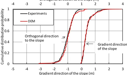
intervals equal to the diameter in the vertical view. Figure 3, which shows the cumulative distribution probability of the arrival distance compared to the experiment, indicates the simulation agrees fairly well with the experiment.
Although this simulation validates our simple model, an additional simulation study based on a real disaster is also used as another validation case.
80 41°
55
55 180
168 350
290
X
Y 91
A box for rocks to be dropped Hinge
Opening and closing
91 50
50 Concrete slope Unit : cm
Figure 1. Description of the experiment by Tochigi et al. Figure 2. Simulation of the simple model
-4 -3 -2 -1 0 1 2 3 4
0 0.2 0.4 0.6 0.8 1
-5 -4 -3 -2 -1 0 1 2 3
Orthogonal direction to the slope (m)
Cu
mu
la
ti
ve
d
is
tr
ib
uti
on
p
ro
b
ab
ili
ty
Gradient direction of the slope (m)
Experiments
DEM
Orthogonal direction to the slope
Gradient direction of the slope
Figure 3
.
Comparison of the cumulative distribution probabilityVERIFICATION
Strictly speaking, DEM calculation software must be verified by sequentially comparing the results obtained by the software to the change in the displacement derived from the numerical integration of the equations of motion. In the context of the simple model proposed in this study and for practical purposes, it is more important to evaluate if the restitution of elements, time intervals for stable calculation results, sliding, and rolling are within the acceptable errors of the theoretical values.
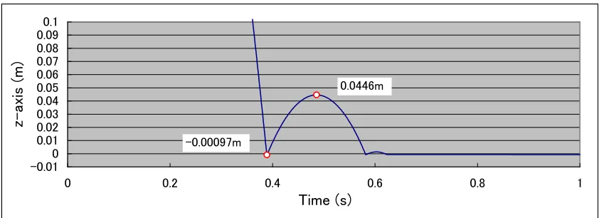
1.Verification of the numerical simulation of the restitution experiment
coefficient, the normal direction of the viscous damping coefficient, and the mass, we verified whether the expected restitution coefficient is observed. Table 1 shows the analysis parameters and the target restitution coefficient.
Figure 5 shows the results of the numerical experiment, while Table 2 shows the results in a table format. The observed values and the theoretical values agree well, validating theoretically that the sound restitution movements occur given the normal direction of the spring coefficient and the normal direction of the viscous damping coefficient. It should be noted that the verification for the tangential direction is omitted since the algorithm is the same as that for the normal direction.
Table 1 Target coefficient of restitution and analysis parameters Target coefficient of
restitution
Element mass (kg) Spring coefficient
(N/m)
Viscous damping coefficient (N·s/m)
0.250 8.78kg 3.67×10⁷ 1.45×10⁴
0.445 8.78kg 3.67×10⁷ 8.96×10³
Table 2 Experimental results Target coefficient of
restitution
h1 *
(m) h2
*
(m) Coefficient of restitution
(observed value)
0.250 0.741 0.046 0.249
0.445 0.741 0.147 0.445
* Interference value δ when the falling element collides with the fixed element must be calculated.
Figure 4. Falling experiment and the coefficient of restitution
1.038 0.204904 -0.1
0 0.1 0.2 0.3 0.4 0.5 0.6 0.7 0.8
0 0.2 0.4 0.6 0.8 1
時間(S)
Z
座標
(m)
-0.010
0.01 0.02 0.03 0.04 0.05 0.06 0.07 0.08
0.090.1
0 0.2 0.4 0.6 0.8 1
時間(S)
Z
座標
(m) 0.0446m
m 0.740m
-0.00097m
Figure 5. Numerical results of the falling experiments
h2
R=v2/v1=(h2/h1)
0.5
(1)
R: Coefficient of restitution
v1: Velocity at the moment before the collision
v2: Velocity at the moment after the collision
h1: Initial height h2: Bounce height
z-ax
is (m)
2.Verification of a numerical simulation of the restitution experiment
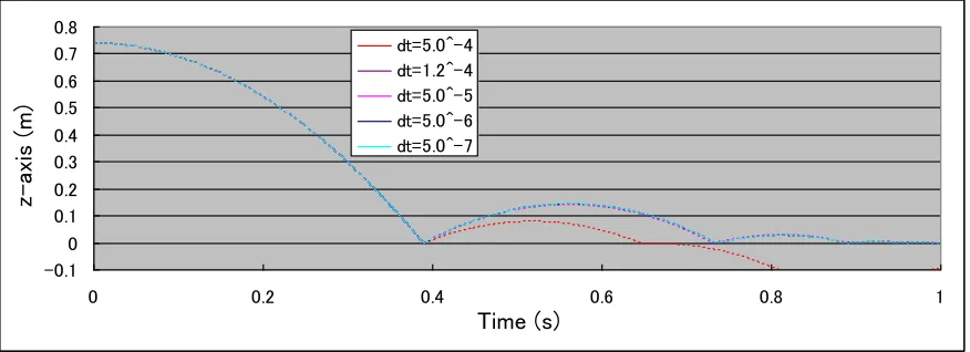
Next, the time interval for the stable calculation results is considered. Based on experience, the time interval dt for stabilized calculation results is expressed as
K m
dt0.25 min /
(4)
Figure 6 shows the result of the parametric study using the time interval as a parameter and the results of the numerical experiment with a restitution coefficient of 0.45, as in Fig. 8. If dt is less than
dt=1.2 ×10⁻⁴, dt is smaller than the value calculated from equation (4), indicating that the solution is not much different. However, if dt is greater than dt = 5.0 × 10⁻⁴, the results show extreme restitution. The analysis shown in Fig. 8 was conducted with dt = 1.2× 10⁻⁴.
-0.1 0 0.1 0.2 0.3 0.4 0.5 0.6 0.7 0.8
0 0.2 0.4 0.6 0.8 1
時間(S) Z 座標 ( m ) dt=5.0^-4 dt=1.2^-4 dt=5.0^-5 dt=5.0^-6 dt=5.0^-7
Figure 6. Time interval parametric study
3.Verification of a numerical simulation involving sliding and rolling
In the initial condition, the spherical element with a 6-cm diameter (white) ball was fixed and the another spherical element with a 6-cm diameter (brown) ball was placed in contact with the surface of the fixed element at an angle of ϕ= 30º (Fig. 7). Then the simulator-generated movements of rolling and sliding were observed. Depending on the strength of friction between the elements, three types of movements are found: rolling without sliding (movement #1), rolling and sliding (movement #2), and sliding without rolling (movement #3). In the three-dimensional context, friction angle θ must satisfy 3 × tanθ > tan ϕ in order for the element to roll without sliding. (In this experiment, θ = ~10°.) The condition to realize sliding without rolling occurs when θ = 0°.
z-ax is (m) Time (s) 0.0000 0.0002 0.0004 0.0006 0.0008 0.0010
0.000 0.005 0.010 0.015 0.020 0.025
変 位 ( m ) 時間(s)
DEM(program(a)):摩擦角0°
DEM(program(a)):摩擦角10°
理論値:転がらずに滑る 理論解:滑らずに転がる C h a ng e i n d i sp la c e me n t (m) Time (s) :Angle of friction 0° :Angle of friction 10° Theoretical solution: sliding without rolling Theoretical solution: rolling without sliding
Figure 7. Initial condition of analysis: Brown element comes in contact with the fixed white element at a 30°angle.
Hence, these three types of movements can be observed under the following conditions:
Movement #1: rolling without sliding (3 × tanθ > tan ϕ) Movement #2: rolling and sliding (0 < 3 × tanθ < tan ϕ)
Movement #3: sliding without rolling (θ = 0°)
Figure 8 shows the results of movements #1 and #3 in the simulation. The x- and y-axes show time and the change in displacement, respectively. For each movement, the simulation results and theoretical solutions agree well.
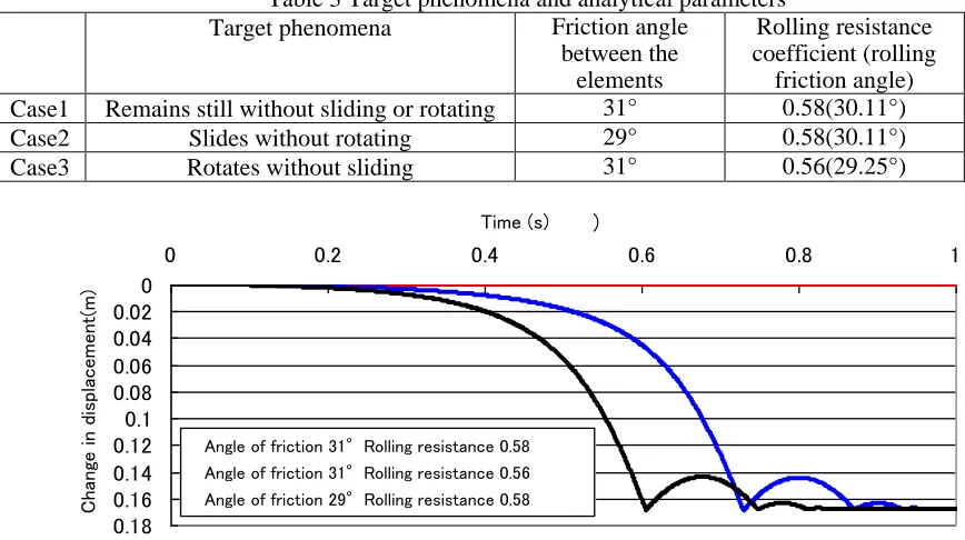
4.Verification of a numerical simulation involving the rolling resistance
Using the same conditions as above (same as Fig. 7), whether the expected movements can be observed is verified given the friction angle between the elements and the rolling resistance coefficient (rolling friction angle). Table 3 shows the target phenomena and analysis parameters. Because the elements are in contact at 30°, both the angle between the elements and the angle of rolling must exceed 30° similar to case 1 in Table 3 in order for the brown element to remain still. In case 2 in Table 3, the friction angle between the elements is less than 30°, while the rolling friction angle is less than 30° in case 3.
Figures 9 shows the simulation results. In case 1, the element does not move, whereas the element slides in cases 2 and 3. Hence, the numerical simulation experiments reproduce the expected phenomena.
Table 3 Target phenomena and analytical parameters
Target phenomena Friction angle
between the elements
Rolling resistance coefficient (rolling
friction angle)
Case1 Remains still without sliding or rotating 31° 0.58(30.11°)
Case2 Slides without rotating 29° 0.58(30.11°)
Case3 Rotates without sliding 31° 0.56(29.25°)
0 0.02 0.04 0.06 0.08 0.1 0.12 0.14 0.16 0.18
0 0.2 0.4 0.6 0.8 1
時間(s)
鉛直
変位
(
m
)
摩擦角31度、転がり摩擦係数0.58 摩擦角31度、転がり摩擦係数0.56 摩擦角29度、転がり摩擦係数0.58
Figure 9. simulation results
VALIDATION
1. Simulation object
At the Nakadori area of Fukushima Prefecture, large-scale slope failures (Nakamura et al., 2012) occurred
during the 2011 Tohoku -Pacific Ocean Earthquake. From the acceleration records of the surroundings,
the maximum acceleration is assumed to be about 300 gal. Figures 10 show the location of this area and collapsed slope site, respectively.
Cha
nge i
n displa
cement
(m)
Time (s)
Figure 10. Collapsed slope site (views of the front, north, and south sides of Route 4)
2. Simulation model
As shown in Figure. 11, the balls are spaced 1.25 m apart in the xy-plane and at heights in the z- direction
based on the numerical elevation model of the Geospatial Information Authority of Japan (GSI) for the
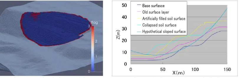
part of the land surface other than the collapsed region. This is the same as the model for the slope and the floor in the simple model shown with the white balls in Figure. 11. The red balls (slip surface particles) indicate the slip surface where the shape is assumed to be a part of the spherical surface. To allow the soil above the slip surface to slip smoothly under its own weight, slip surface particles with 1.25-m diameters are spaced densely at regular intervals of the partical radius on the xy-plane. In this study, the shape of the slip surface is approximated as a circular arc in the two-dimensional model and the part of spherical surface in the three-dimensional model. In the future, it is necessary to verify the consistency with the actual slip situation. A group of blue balls (soil balls) indicates the collapsed area, including the ground surface before collapse.
Figure 12 shows the cross section of the collapsed area. Regarding the position assumption of the slip
plane, a general method is to use the circular slip method for stability analysis of the slope or FEM
analysis. However, to quickly determine the slip plane, herein we assume that this slip plane passes through the positions of the bottom of the collapsed slope and the top of embanked slope surface (the shoulder of the former embanked surface). Based on this slip plane, the slip surface is assumed to be a spherical surface that contains as much of the old embankment as possible with a minimal dip in the foundation. In practice, how to determine the slip surface for a cross section of the mentioned damaged is unknown.
Table 4 and 5 show the parameters for the balls and their contact for the basic case, respectively. Using these values, the restitution coefficients both between soil/soil balls (blue) and between soil/slip surface balls (red) are 0.48. This finding is consistent with the simulation result in Fig. 3. In other words, the collapsed soil is represented by an assembly of sample particles that are the same as those used in the experiment of Fig. 2 and with the same restitution coefficient. The restitutions between the collapsed soil and the ground surface, roads, etc. are considered small. Thus, the coefficient between the soil particles (blue) and the field particles (white) is set to 0.1. Meanwhile, the friction angle between soil (blue) and slip surface particles (red) is set to 0 to initiate the soil collapse by its own weight.
Figure 11. Simulation model Figure 12. Cross section and slip line Base surfasce
Table 4 Contact parameters between the balls
Particles of the ground model (blue) or Blue particle and sliding surface
particle (red)
Particle of the ground model (blue) and a field
particle (white)
Radial spring coefficient (m/N) 1.96×10⁹ 1.96×10⁹
Tangent spring coef. (m/N) 1.96×10⁹ 1.96×10⁹
Radial viscous damp. coef. (m/N/s) 1.19×10⁶ 3.09×10⁶
Tangent viscous damp. coef. (m/N/s) 1.19×10⁶ 3.09×10⁶
Friction angle (°) 30,0 30
Table 5 Ball parameters
Particle radius (m) 0.625
Density (kg/m3) 3411.4
3. Simulation results
Figures 13 show the results of simulated slip shape where the actual collapsed soil surface is added for comparison. Since the area of the assumed slip surface in the simulation is larger than the actual slip surface, the deposited soil range is wider by about a factor of two. However, considering that the results are obtained based on a simple analytical model from the information of one geological section of the
collapsed soil and a GSI numerical elevation as well as the determined property of the restitution
coefficient between the collapsed soil and ground is 0.1, the results are useful. It should also be noted that the results provide a conservative estimated range of the deposited soil area.
Many application problems contain less information (soil layers and properties, etc.) about the target site than the present study. Often crucial information about the positions of both the slip top and bottom are unknown prior to collapse. Consequently, an appropriate modeling method may be necessary for such cases.
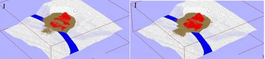
Thus, we simulated the results using the codes for two DEMs developed by J and I Company.
Although the traveling distance of the collapsed soil is slightly larger using I Company’s code, the
difference in the results seems insignificant.
Despite the fact that both codes use the same analysis conditions, the results do not completely match. We believe that this difference is due to the calculation scheme (e.g., time integration), which differs between the two codes because the effect accumulates over the tens of thousands of calculation steps,
especially for strong nonlinear problems with many bifurcation points.
Figure 13. Collapsed slope shape calculated by the code of J and I Company (Red: Actual collapsed surface)
PARAMETERS STUDY
In the previous chapter, we applied the simple model to conservatively calculate the traveling distance of
the collapsed soil. However, from the viewpoint of estimating the volume of collapsed soil, it may be
difficult to say this result is also on safe side. In this chapter, we carried out a parametric study focusing
on the rolling resistance to control the amount of deposits.
1.Results of collapsed slope analysis by a parameters study
Figure 14 shows the analysis results for the mentioned collapsed slope using the rolling resistance
coefficients in Table 3. The larger the rolling resistance coefficient, the smaller the outflow amount of soil
becomes. A rolling resistance coefficient of 0.1 reproduces the actual damage where the collapsed soil
almost did not arrive over Route 4.
Rolling resistance 0.0 Rolling resistance 0.05 Rolling resistance 0.1 Figure 14. Simulation results
2.Evaluation of the amount of collapsed soil
Since the actual amount of collapsed soil that needs to be removed from the road at each site is unknown, the evaluation method proposed here allows the volume to be calculated from each mesh after dividing the target area into meshes as shown in Figure 15. By supposing the angle of the slipped line in the cut
section is 30°, the total collapsed volume as the sum calculated from each mesh is 14,225 m3. The
simulation results of the amount of collapsed soil calculated from J Company’s code and I Company's code are similar.
Table 5 shows the calculation results in the simulation where the maximum amount of collapsed soil
is 26,009 m3 with a rolling resistance coefficient of 0.05 using J Company's code, but is 22,114 m3 with a
rolling resistance coefficient of 0.0 using I Company's code. Although the trends differ between the two
codes, they both produced maximum values that exceed the actual value in the collapsed site. A method to perform a parametric study within an appropriate range is realistic to obtain a maximum value because generally all information is unavailable for the target site (layers, properties, groundwater level, etc.) or cannot be obtained in case of an emergency.
Table 5 Amount of soil to be removed (m3)
Actual damage Rolling resistance
coefficient
0.0 0.05 0.10
14,225 Company J 24,048 26,009 22,340
Company I 22,114 18,262 14,490
Figure 15. Estimated amount of soil removed from the road in an actual disaster Cut surface
CONCLUSION
We verified and validated the proposed simple model. Additionally, we showed that using the maximum value from a parametric studying involving the rolling friction as an estimate to determine the amount of soil to be removed from the inner road after the collapse is suitable. The calculated values by two different simulation software programs were more conservative than the actual data.
The value of the restitution coefficient between the particles is unclear in the analysis parameters. Nonetheless, we believe that the value range of the restitution coefficient between the particles is limited, and the maximum possible value of the coefficient can be used to correctly estimate the area via a parametric study. However, it is important to repeat the reconstruction analysis to improve reliability of the validation in the future.
Acknowledgement
We would like to thank Dr. Susumu Nakamura, College of Engineering, Nihon University for providing valuable resources regarding the Asahidai disaster. This study was conducted as a part of the working activities of the Mini-Committee of Japan Society of Civil Engineers Nuclear Committee for Advancement of Ground Stability Analysis.
REFERENCES
Atomic Energy Society of Japan, A standard for Procedure of Seismic Probabilistic Risk Assessment (PRA) for nuclear power plants: 2007.
Japan Nuclear Energy Safety Organization, Guideline for Design and Risk Evaluation against the Seismic Stability of the Ground Foundation and the Slope. JNES-RE-2013-2037: 2013.
H. Nakase, CAO. G, K. Tabei, H. Tochigi, T. Matsushima, A Method to Assess Collision Hazard of Falling Rock Due to Slope Collapse Application of DEM on Modeling of Earthquake Triggered Slope Failure, Journal of Japan Society of Civil Engineers, Ser. A1 (Structural Engineering & Earthquake Engineering (SE/EE)) Vol. 71,No. 4, I_476-I_492: 2015.
Cundall, P.A, A Computer Model for Simulating Progressive, Large Scale Movement in Blocky Rocksystem, symp.ISRM, Nancy France, Proc., Vol2,pp.129-136: 1971.
Cundall, P.A, Strack, O.D.L, A discrete numerical model for granular assembles, Geotechnique 29, pp.47-65: 1979.
H. Nakase, T. Kurita, T. Annaka, F. Katahira, T. Kyono, Simulation of plane strain compression test by an improved individual element technique, Japan Society of Civil Engineers 1991 Annual Meeting, Vol3, pp.466-467: 1991.
Ai, J., J. F. Chen, J. M. Rotter, and J. Y. Ooi, Assessment of Rolling Resistance Models in Discrete Element Simulations, Powder Technology,206, 269-282: 2011.
Wensrich, C. M., and A. Katterfeld, Rolling Friction as a Technique for Modelling Particle Shape in DEM, Powder Technology, 217, 409-417:2012.
Sakaguchi, H., Ozaki, E. & Igarashi, T. , Plugging of the Flow of Granular Materials during the Discharge from a Silo, Int. J. Mod. Phys. B, 7, pp.1949-1963:1993.
Tochigi H Ootori Y Kawai T Nakajima M and Ishimaru M. ,Investigation of Influence Factor concerned with Traveling Distance-Development of Influence Area Prediction Method by Shaking Table Test of Slope Failure and Two Dimensional Distinct Element Analysis. Civil Engineering Research Laboratory Rep.No.N08084: 2009.
Nakamura S Sentoh N Umemura J OTsuka S Toyota K,The geotechnical disaster in Nakadoori area and Iwaki area of Fukushima Prefecture- Failure and deformation of embanked ground and natural slope,