Modifying the Schwarz Bayesian Information Criterion to Locate Multiple Interacting Quantitative Trait Loci



DOI: 10.1534/genetics.103.021683

Modifying the Schwarz Bayesian Information Criterion to Locate Multiple

Interacting Quantitative Trait Loci

Małgorzata Bogdan,*

,†

_{Jayanta K. Ghosh}

†,‡

_{and R. W. Doerge}

†,§,1

*Institute of Mathematics, Wroclaw University of Technology, 50-370 Wroclaw, Poland,‡_{Indian Statistical Institute, Calcutta 700035, India,} †_{Department of Statistics, Purdue University, West Lafayette, Indiana 47907 and}§_{Department of Agronomy, Purdue University,}

West Lafayette, Indiana 47907 Manuscript received August 27, 2003 Accepted for publication March 5, 2004

ABSTRACT

The problem of locating multiple interacting quantitative trait loci (QTL) can be addressed as a multiple regression problem, with marker genotypes being the regressor variables. An important and difficult part in fitting such a regression model is the estimation of the QTL number and respective interactions. Among the many model selection criteria that can be used to estimate the number of regressor variables, none are used to estimate the number of interactions. Our simulations demonstrate that epistatic terms appearing in a model without the related main effects cause the standard model selection criteria to have a strong tendency to overestimate the number of interactions, and so the QTL number. With this as our motivation we investigate the behavior of the Schwarz Bayesian information criterion (BIC) by explaining the phenome-non of the overestimation and proposing a novel modification of BIC that allows the detection of main effects and pairwise interactions in a backcross population. Results of an extensive simulation study demonstrate that our modified version of BIC performs very well in practice. Our methodology can be extended to general populations and higher-order interactions.

P

OPULAR methods for mapping quantitative trait sional genome searches as a means of mapping epistatic loci (QTL) include interval mapping (Landerand QTL. In particular they proposed an interesting exten-Botstein 1989), composite interval mapping (Zeng sion of MQM by addressing a crucial problem pertaining 1993, 1994) and multiple QTL mapping (MQM;Jansen to the choice of marker cofactors. By including all avail-1993;JansenandStam1994). These statistical methods able markers in a regression equation and using a Bayes-do not allow the location of QTL in situations when ian approach to penalize large values of the correspond-there are no main effects for the respective QTL, but ing regression coefficients many of the previously there are (epistatic) interactions with other QTL mentioned issues are eliminated. The disadvantage of (genes) that influence the quantitative trait. Epistatic this method is that, when detecting epistatic QTL, it QTL are known to play important roles in many disease requires the choice of “the effective dimension” (i.e., studies, such as cancer (Fijneman et al. 1996, 1998), number of QTL) for epistatic interactions, which has and it is also suspected that they play a key role in the strong influence on the power of detection.

evolutionary process (Wolfet al.2000). An alternative way to approach the problem of

map-A direct solution to detecting epistatic QTL is to ping epistatic QTL relies on developing new methods search for several QTL simultaneously and fit an appro- for reducing the numerical complexity of MIM. In re-priate multiple regression model with interactions. cent work Carlborg et al. (2000), Nakamichi et al.

However, the utility of such an approach, which is re- (2001), and Broman and Speed (2002) use random ferred to as a multidimensional version of interval map- search methods to accelerate the search over the class ping, called multiple interval mapping (MIM;Kaoet al. _{of possible multidimensional models. The results from}

1999), is limited by two interconnected issues. The first _{their approach hold great potential for further progress} is the requirement of deciding how many terms (main _{in solving the problem of the computational complexity} effects and epistasis) should be included in the model. _{of MIM.}

The second issue is the computational complexity of _{Regardless of which method we use to search the}

the search over the space of possible multidimensional _{genome for QTL we need to solve the problem of} esti-models. To avoid these problemsJanninkandJansen _{mating QTL number, which in turn directly affects the} (2001) and Boer et al. (2002) proposed one-dimen- _{dimensionality of the model space. The standard way of} deciding how many main and interacting (QTL) effects should appear in the model relies on using many

statisti-1_{Corresponding author:Department of Statistics, 1399 Math Bldg.,}

cal tests (see Kao et al. 1999). A disadvantage of this

Purdue University, West Lafayette, Indiana 47907.

E-mail: [email protected] approach is that it allows the comparison of only nested

models. It is also unclear how to adjust the significance mate the model dimension. To address this issue we follow the approach suggested byBall(2001) and pro-thresholds for each consecutive test.

Model selection criteria have been used as an alterna- pose an easy modification of BIC that relies on taking into account the realistic prior distribution on the set tive approach for the problem of model selection in

QTL mapping. Two easy-to-compute model selection of compared models. In comparison toBall(2001) we

extend the method to cover models with interactions criteria that are often employed in statistics are the

Akaike information criterion (AIC;Akaike1974) or the and calibrate the prior to gain the control over the type I error of our procedure. An extensive simulation study Schwarz Bayesian information criterion (BIC;Schwarz

1978). These criteria belong to the family of the so- verifies that our proposed criterion deals very well with the problem of overfitting the model and allows the calledpenalized maximum likelihood methodsand are based

on the recommendation of choosing the model for detection of main effects and pairwise interactions in a backcross population. While our proposal is based on which the likelihood of the data minus the penalty for

the model dimension obtains the maximal value. These QTL mapping in a backcross population, our methodol-ogy can be extended to general populations and to criteria were used by Jansen (1993) and Jansen and

Stam(1994) to choose marker covariates for MQM and higher-order interactions. byPiephoandGauch(2001),Nakamichiet al.(2001),

Ball(2001),BromanandSpeed(2002), andSiegmund

METHODS (2003) to directly estimate QTL number. For a review

and discussion of model selection methods as applied Consider a backcross population where qij denotes

to QTL mapping seeBaldinget al.(2002) orSilanpa¨a¨ the genotype of theith individual at thejth QTL:qij⫽

andCorander(2002). ⫺1_⁄

2if theith individual is homozygous at the jth QTL PiephoandGauch(2001) investigated many model and qij ⫽ 1⁄2 if it is heterozygous. We assume that the selection criteria via simulation. In their study different relationship between the trait valueYiand QTL

geno-criteria were used to choose pairs of markers flanking types is given by a normal regression model, QTL. Their results suggest that out of the considered

Yi⫽ ␮ ⫹

兺

m

j⫽1

␤jqij ⫹

兺

1ⱕj⬍lⱕm

␥jlqijqil⫹ εi, (1)

criteria BIC has the best properties and can be recom-mended for the estimation of the number of QTL with

main effects.BromanandSpeed(2002), however, rec- where m is the QTL number andεi ⵑ N(0, ␴2) is the

environmental noise. The second summation in our ommend a modification of BIC to select markers

strongly associated with the trait. Contrary to Piepho model corresponds to pairwise epistatic interactions. The formulation of the model allows some of the coeffi-andGauch(2001) they use BIC to choose single

mark-ers instead of pairs.BromanandSpeed(2002) observe cients␤jand␥jlto be zero to accommodate cases when

there are QTL that are not involved in epistatic effects. that in this situation the original BIC has a tendency to

overestimate the QTL number. To solve the problem It also addresses the scenario when QTL might not have their own main effects, yet influence the quantitative of the overfitting they propose a modification of BIC,

with a larger penalty for model dimension. Simulations trait by interacting with other genes, (i.e., epistasis). Later we usepto denote the number of QTL with main reported inBromanandSpeed(2002) show that their

modified version of BIC performs very well and detects effects andqto denote the number of nonzero epistatic terms.

the correct model more often than composite interval

mapping does (Zeng1993, 1994). We rely on MIM (Kaoet al.1999) to simultaneously

locate multiple QTL. This method requires fitting the While both of the methods put forth byPiephoand

Gauch(2001) andBromanandSpeed(2002) can be model (1) for a dense grid of possible QTL positions. For each of the possible genomic locations the geno-used to estimate the number of QTL with main effects,

they do not generalize directly to the situation where types of the putative QTL are inferred using the geno-types of flanking markers and the EM algorithm interaction terms appear in the model. Our extensive

simulations (Bogdan andDoerge 2003) showed that (Dempsteret al.1977) is employed to estimate parame-ters of the model (1). The locations for which the fitted the phenomenon of overfitting becomes even more

sig-nificant when we allow interaction terms to appear in model yields the largest likelihood are subsequently chosen.

the model without the related main effects.

In the present work we concentrate on BIC, which, A first step in the reduction of the complexity of MIM sometimes relies on identifying interesting genomic re-according to the QTL simulation study ofPiephoand

Gauch(2001) and our independent simulations, per- gions on the basis of an initial, relatively coarse search. In the Bayesian setting this approach was suggested by forms better than other popularly used model selection

criteria. In particular, we recall the Bayesian roots of Sen and Churchill(2001), who used an initial scan based on a 10-cM pseudo-marker grid. However, for the BIC and explain the reasons why this criterion, when

approach is to base the initial search on the net of where RSS is the residual sum of squares from

regres-marker positions and then use more refined methods sion.

(e.g., MIM) to search in the neighborhood of the chosen Rationale for modifying BIC: Broman and Speed markers. Ball(2001), Broman and Speed (2002), Yi (2002) report that the original BIC, when used to select

et al. (2003a), andXu (2003) successfully search over single markers with significant main effects, has a

ten-markers to locate multiple QTL and are justified in dency to overestimate QTL number. On the basis of doing so on the basis of the fact that flanking markers work not shown here (BogdanandDoerge 2003) we absorb all the information associated with the QTL have found that the tendency to overestimate QTL

num-(Whittakeret al.1996). ber becomes more significant when the portion (or

If we reduce MIM to a search over markers, then the entirety) of the genome under investigation increases. problem of the QTL location reduces to the problem To understand this further we compare the rates at

of choosing the best model of the form which the number of different models increases as the

number of available markers increases. Our rationale

Yi⫽ ␮ ⫹

兺

j僆I

␤jXij⫹

兺

(u,v)僆U

␥uvXiuXiv⫹εi, (2)

is based on the observation that the number of possible models of the particular form (2), involvingkdistinct whereXij denotes the genotype of theith individual at

markers, is equal to

冢

Nm

k

冣

, whereNmis the total number

thejth marker;I is a certain subset of the setᏺ⫽ {1,

. . . ,Nm}, whereNmis the number of available markers; of available markers. Thus, whenkis much smaller than

Nm, the number of models involvingkmarkers increases and U is a certain subset of ᏺ ⫻ ᏺ. For a backcross

with Nm approximately like Nmk. The difference in the population the random variablesXiuXiv correspond to

numbers of possible “small” and “large” models in-the epistatic terms that are not correlated to any of in-the

creases quickly withNm, and for largeNmthe probability main effects. In particular, XiuXiv is not correlated to

either Xiu or Xiv even if the uth and vth markers are of choosing models with many components, just by

ran-statistically dependent via linkage. Thus, the epistatic dom chance, is relatively high. Furthermore, for a large effects are statistically not confounded with any of the number of interaction terms, Bogdan and Doerge main effects, and in most cases they will be detected (2003) show that the original BIC has a tendency to only if the epistatic interactions are present. choose models with epistatic terms even when in reality

One difficulty in fitting model (2) is the estimation there is no epistasis.

of the number of main effects and interaction terms to The phenomenon of overestimation itself suggests be included in the model. There is a vast statistical _{the way the standard model selection criteria should} literature on the choice of the number of terms in a _{be modified to make them useful for QTL mapping.} linear model (seeMiller1990 orMcQuarrieandTsai _{Namely, the high rate at which the number of} multidi-1998) and there are many model selection criteria that _{mensional models increases, when the number of} avail-can be used for this purpose. As mentioned earlierBro- _{able markers increases, suggests that the penalty for the} manandSpeed(2002) andPiephoandGauch(2001) _{model dimension should increase with this number.} recommend using the Schwarz BIC (Schwarz1978) to _{This condition is satisfied, for example, by criteria}

pro-estimate the number of QTL with main effects. In a _{posed by Broman and Speed (2002) and Siegmund}

general statistical context BIC recommends choosing _{(2003). Second, the fact that there are many more}

inter-the model that maximizes inter-the expression _{action terms than the main effects suggests that the}

penalty for including an interaction should be larger

S⫽log L(Y|␪)⫺1

2klogn, (3) than the penalty for including a main effect. Following

these two suggestions we modify BIC by supplementing where ␪ is the vector of model parameters, L(Y|␪) is _{it with a realistic prior distribution on the set of possible} the likelihood of the data,kis the number of parameters _{models. Taking advantage of the fact that BIC is the} (dimension of␪), andnis the sample size. BIC belongs _{approximation to the Bayesian rule for the choice of} to the wide class of the so-called penalized maximum- _{the “best” model we denote by␪}

i ⫽ (␮,␤1, . . . ,␤p(i), likelihood methods and the second term in this crite- _␥

1, . . . ,␥q(i),␴) the vector of parameters of theith linear rion,1_⁄

2klogn, is called the penalty for the complexity _{model, M}

i, given by Equation 2. Here p(i) and q(i)

of the model. An important advantage of BIC is that

denote the number of main effects and interaction for a wide range of statistical problems, and in particular

terms involved inMi. We assign a certain prior

distribu-for multiple regression, it is consistent (i.e., when the

tion for ␪i and denote the density of this distribution

sample size grows to infinity, the probability of choosing

byf(␪i). Moreover, let us denote the prior probability

the right model converges to 1). In the context of linear

of theith model by␲(i). Given thatL(Y|␪i,Mi) denotes

regression, maximizingSis equivalent to minimizing

the likelihood of the data given the vector of parameters

␪i, letp(Y|Mi) denote the likelihood of the data given

BIC⫽n log

冢

RSS

p(Y|Mi)⫽

冮

L(Y|␪i,Mi)f(␪i|Mi)d␪i. (5) ␯to the event that thejth interaction term appears in the

model. Our prior distribution assumes that particular The posterior probability of the ith model, given the _{terms enter the model independently of others and for}

data, is _{a particular model Mi involving p(i) main effects and}

q(i) interactions we obtain

P(Mi|Y)⫽

␲(i)p(Y|Mi)

兺

l

j⫽1␲(j)p(Y|Mj)

, (6)

␲(Mi)⫽ ␣p(i)␯q(i)(1⫺ ␣)Nm⫺p(i)(1⫺ ␯)Ne⫺q(i).

This choice of prior implies that the prior distributions wherelis the number of possible models.

on the number of main effects and epistatic terms are The Bayesian rule recommends choosing the model

binomial with parametersNmand␣, andNe and␯, re-for which the posterior probabilityP(Mi|Y) is the largest

spectively. (seeSchwarz1978). Since the denominator in

Equa-For simplicity we consider ␣ and␯ as␣ ⫽ 1/l, ␯ ⫽ tion 6 is the same for all considered models, Bayes’ rule

1/u, where l and u are certain natural numbers, and recommends choosing the model for which␲(i)p(Y|Mi)

restate the prior distribution as is the largest. The BIC criterion neglects the prior

proba-bilities␲(i) of different models and approximates log _log␲(M

i)⫽C(Nm,Ne,l,u)⫺p(i)log(l⫺1)

p(Y|Mi) by logL(Y|␪ˆi,Mi)⫺1⁄2(p(i)⫹q(i)⫹2)logn,

⫺q(i)log(u⫺1), where␪ˆiis the maximum-likelihood estimator of␪i, and

p(i)⫹q(i)⫹2 is the number of estimated parameters

where C(Nm, Ne,l, u) is a constant dependent on Nm, [i.e., p(i)⫹ q(i) for main and epistatic effects, and 2

Ne,l, and u. Incorporating this prior distribution into for␮and␴]. Neglecting␲(i) corresponds to assigning

the BIC [modified Schwarz BIC (mBIC)] allows the the same prior probability to all considered models.

following rule: choose the model that minimizes While in many applications this approach is well

justi-fied, in the context of QTL mapping it lends itself to _{mBIC(i)⫽nlog RSSi⫹ (p(i)⫹q(i))log n⫹2p(i)} assigning unrealistically high prior probabilities to the

⫻ log(l⫺ 1)⫹2q(i)log(u⫺ 1). (8) events where many regressors are involved [e.g., when

200 markers are available, the number of different mod- _{The expected values of the prior distribution for the} els involving 100 main effects is

冢

200

100

冣

⬇9.05⫻10 58_and

number of main effects are equal toNm/landNe/ufor the number of interaction terms. Therefore, since the the prior probability of the event that 100 regressors

are involved is⬎1056_{times larger than the prior proba- choice of l andu should reflect our prior knowledge} bility of the event that there is just one regressor]. Moti- on the QTL number, the values of land u should be vated to improve on this we suggest supplementing BIC relatively small when we expect many QTL and large with a more realistic prior distribution,␲, on the class when we expect only few. Extensive simulations were of possible models, and choosing the model for which performed for the purpose of investigating the standard values oflanduwhen we have no prior knowledge on

S˜(i)⫽log␲(i)⫹logL(Y|␪ˆi,Mi)

the QTL number. We letlandutake on values in such a way that for the sample sizesnⱖ200 the probability

⫺ 1

2(p(i)⫹ q(i)⫹ 2)logn (7) of type I error (detecting at least one QTL when there are none) does not exceed 5%. We observed that when

obtains a maximum. _{markers are densely spaced (distance between markers}

In the context of multiple regression _{is not⬎20 cM) we can obtain our aim by keeping the}

expected values of the number of main effects and inter-logL(Y|␪ˆi,Mi)⫽ ⫺

n

2log RSSi ⫹C(n), action terms at a constant level close to 2. In particular, and as is seen next, in our simulations we used values where C(n) is the constant dependent only on n, and l⬇Nm/2.2 andu⬇Ne/2.2. In theappendixwe present maximizing (7) is equivalent to minimizing the quantity results of some theoretical calculations that support our empirical choice of l and u. These calculations yield

S(i)⫽ nlog RSSi ⫹(p(i)⫹ q(i))logn⫺ 2 log␲(i).

approximate bounds on the type I error of our proce-dure and demonstrate that the proposed choice of l

Prior distribution␲:AssumeNmmarkers are available,

andusolves the problem of multiple comparisons and and thereforeNmpotential regressors andNe⫽(Nm(Nm⫺

allows control of the type I error. In comparison to 1))/2 potential interaction terms. The number of all

the original BIC the penalty in our proposed/modified models of the form (2) that can be constructed using

criterion involves additional terms 2p(i)log((Nm/2.2)⫺1)

subsets ofNmmarkers is equal to 2Nm⫹Ne. To assign prior

and 2q(i)log((Ne/2.2)⫺1). A similar additional penalty probabilities to these models we follow the standard

appears in the criterion proposed bySiegmund(2003), solution proposed inGeorgeandMcCulloch(1993).

who approaches the problem of QTL mapping differ-Namely, we assign the probability ␣ to the event that

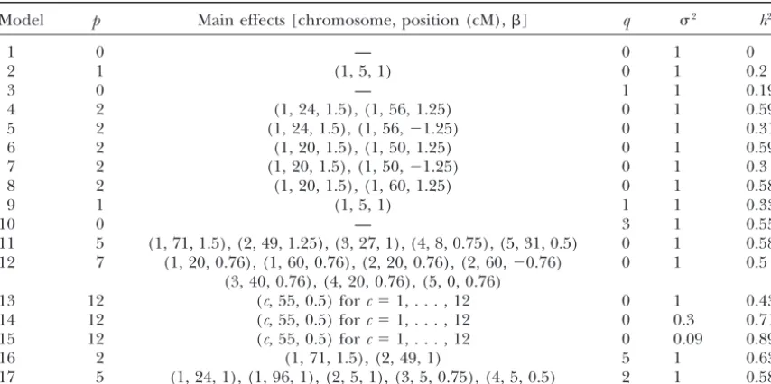
TABLE 1

Simulation models

Model p Main effects [chromosome, position (cM),␤] q ␴2 _h2

1 0 — 0 1 0

2 1 (1, 5, 1) 0 1 0.2

3 0 — 1 1 0.195

4 2 (1, 24, 1.5), (1, 56, 1.25) 0 1 0.59

5 2 (1, 24, 1.5), (1, 56,⫺1.25) 0 1 0.31

6 2 (1, 20, 1.5), (1, 50, 1.25) 0 1 0.59

7 2 (1, 20, 1.5), (1, 50,⫺1.25) 0 1 0.3

8 2 (1, 20, 1.5), (1, 60, 1.25) 0 1 0.58

9 1 (1, 5, 1) 1 1 0.33

10 0 — 3 1 0.55

11 5 (1, 71, 1.5), (2, 49, 1.25), (3, 27, 1), (4, 8, 0.75), (5, 31, 0.5) 0 1 0.58 12 7 (1, 20, 0.76), (1, 60, 0.76), (2, 20, 0.76), (2, 60,⫺0.76) 0 1 0.5

(3, 40, 0.76), (4, 20, 0.76), (5, 0, 0.76)

13 12 (c, 55, 0.5) forc⫽1, . . . , 12 0 1 0.43

14 12 (c, 55, 0.5) forc⫽1, . . . , 12 0 0.3 0.71

15 12 (c, 55, 0.5) forc⫽1, . . . , 12 0 0.09 0.89

16 2 (1, 71, 1.5), (2, 49, 1) 5 1 0.63

17 5 (1, 24, 1), (1, 96, 1), (2, 5, 1), (3, 5, 0.75), (4, 5, 0.5) 2 1 0.58

The number of QTL with main effects␤jis denoted byp, andqis the number of epistatic terms with effects

␥jl, as defined in model (1). The environmental noise is denotedεiⵑN(0,␴2). Broad sense heritability ish2,

and the epistatic effects are as described in Table 2.

additional terms make our criterion similar to the risk Miller1990) is used to search the space of possible multidimensional models. At each consecutive step we inflation criterion (RIC) proposed by Foster and

George (1994) in which the penalty for including k test all terms (main and interaction) not yet in the model and choose the one whose presence in the model orthogonal regressors is equal to 2klogt, wheretis the

total number of available regressors. Note, however, that yields the lowest value of the modified BIC criterion (Equation 8; mBIC). To save computational time the whenntends to infinity these additional terms are

over-shadowed by the BIC penalty (p(i)⫹ q(i)) log nand, procedure is stopped after 30 steps and the resulting 31 models are evaluated on the basis of minimizing the contrary to RIC, our criterion has the asymptotic

proper-ties of the BIC (i.e., consistency). mBIC (Equation 8). The number of steps is restricted

to 30 since the largest model we use in the simulations has only 12 terms. Actually, we observe that for all the SIMULATIONS cases that we considered, the mBIC criterion was mini-mized by models with ⬍20 terms and that increasing We employ computer simulations to evaluate the

ap-the number of steps above 20 had no influence on ap-the plicability of our proposed modification to the BIC

crite-results. However, in real data studies, when one does rion. Marker and QTL genotypes are simulated for a

not want to bound the QTL number, we suggest using backcross population using 12 chromosomes of the

a larger number of steps. length 100 cM for sample sizesn⫽ 200 andn ⫽500.

The number of QTL with main effects ranges between 0 and 12, and the number of epistatic terms between 0

RESULTS and 5 (Tables 1 and 2). Models 4, 5, and 11–14 (Table

1) are included to allow for a direct comparison to the The results of searching over 1, 5, and 12 100-cM chromosomes, respectively, with markers spaced every results ofBroman andSpeed (2002), as indicated by

model 12, and to the results of Piepho and Gauch 10 cM are shown in Tables 4–6, while Table 7 reports the results for varying marker distances. The number (2001; models 4, 5, 11, 13, and 14). Since we are

inter-ested in how our proposed criterion adjusts to the num- of correctly identified terms (corr. id. ), averaged across 100 simulations, and the average number of false posi-ber of available markers, we search for QTL over 1, 5,

and 12 chromosomes and use marker spacings of 5, tives (extr. ) are reported. The false positives that occur are divided into categories depending on their linkage 10, and 20 cM. The number of available markers and

interaction terms, as well as the corresponding values to true QTL. Following PiephoandGauch(2001) we classify the main effect to be correct if it corresponds of l andu for each of these experiments, is specified

TABLE 2

Details of epistatic effects employed in simulation (Table 1)

Model q Epistatic effects (QTL1; QTL2;␥)

3 1 (1, 5; 1, 90; 2)

9 1 (2, 5; 3, 5; 2)

10 3 (1, 71; 2, 49; 3), (3, 27; 4, 8; 2.5), (5, 31; 6, 35; 2)

16 5 (3, 27; 4, 8; 2.5), (5, 31; 6, 35; 2), (7, 5; 8, 5; 1.5), (9, 5; 10, 5; 1), (11, 5; 12, 5; 0.75)

17 2 (5, 5; 6, 5; 2), (7, 5; 8, 5; 1)

QTLi(i⫽ 1, 2) denotes the position of theith QTL (chromosome and QTL location). The number of epistatic terms and their effects are denoted byqand␥, respectively, and are as described in model (1).

two markers from the neighborhood of one QTL are proposed criterion quickly improve with increasing sam-ple size. Therefore, the accuracy of detecting small mod-chosen, one of these markers is arbitrarily classified as

extraneous. Epistatic terms are classified as correct if els increases (see models 1, 6, and 7 in Table 4) as does the ability to correctly identify models with larger both markers involved lie within 15 cM of the true QTL.

For the no-QTL model (1) the percentage of replicates numbers of QTL (see models 12, 13, 16, and 17 in Table 4). We are aware that the chance of correctly identifying for which the model with no QTL was chosen is

re-ported. While the 15-cM margin is somewhat arbitrary QTL depends on its heritability. In other words, when the variance of the error is equal to 1.0 and the sample it accommodates our situation well and illustrates the

performance of our criterion. Recall that our main goal size isn⫽200, our criterion usually detects main effects with coefficients␤ ⱖ0.76 (the heritability of the single is the estimation of QTL number and not the precise

location of QTL. If we use a narrower range (i.e.,⬍15 QTL with such a␤is 0.13) and interaction terms with

␥ ⱖ 2 (broad sense heritability of 0.20 with just one cM), then some of the properly identified terms will be

classified as extraneous due to the relatively large error such epistatic term in the model) even when they appear in larger models. When the sample size is increased to of localization of weak QTL that is inherent to all QTL

mapping procedures. n⫽500 our criterion usually detects main effects with

␤ ⱖ0.50 (individualh2ⱖ _{0.06) and interaction terms} Our modification to BIC performs very well (Tables

4–7) in practice, adjusts appropriately to the number with␥ ⱖ1.5 (individualh2ⵑ_{0.12). The proposed} crite-rion (mBIC) works particularly well if QTL are located of available markers under consideration, and rarely

overestimates. Furthermore, in all of the examples we close to markers (compare models 4 and 6, and 5 and 7, in Tables 4–6 and models 4 and 8 in Table 7). When considered the probability of incorrectly detecting at

least one QTL, when there are none, does not exceed QTL are located in the middle of an interval defined by two markers it is sometimes the case that both flanking 0.06 and the average number of extraneous QTL, which

are not linked to true QTL, rarely exceeds 0.10. We also markers are chosen, which partially explains the rela-tively large number of falsepositives for models 4 and observe that the average number of extraneous epistatic

terms never exceeded 0.05. This confirms our expecta- 15. An additional reason for the sometimes larger num-ber of extraneous linked QTL is a statistical error of tions that in the backcross population epistatic effects

are usually detected only when they really exist. Since localization of weak QTL. In some cases the correct model was appropriately identified, but the chosen we set the expected values of the prior distribution for

the number of main effects and interaction terms to be markers were slightly farther apart from the true QTL than our set limit of 15 cM. On the basis of this reasoning equal to 2.2, our criterion more easily identifies models

with a small number of terms. The properties of our some of thefalsepositives correspond to correctly

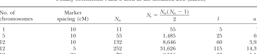
identi-TABLE 3

Penalty coefficientslanduused in the modified BIC (mBIC)

No. of Marker

chromosomes spacing (cM) Nm

Ne⫽

Nm(Nm⫺1)

2 l u

1 10 11 55 5 25

5 10 55 1,485 25 675

12 10 132 8,646 60 3,930

12 5 252 31,626 115 14,375

12 20 72 2,556 33 1,162

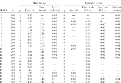
TABLE 4

Results from 100 simulations that each search over 12 100-cM chromosomes with markers spaced every 10 cM

Main terms Epistatic terms

Extr. Extr. Extr. both Extr. one Extr.both

Model n p Corr. id. linked unlinked q Corr. id. linked linked unlinked

1 200 0 0.95 — 0.03 0 — — — 0.02

1 500 0 0.99 — 0.01 0 — — — 0.00

2 200 1 1.00 0.01 0.02 0 0.00 0.00 0 0.02

3 200 0 — 0.00 0.01 1 0.95 0.01 0.00 0.01

4 200 2 1.97 0.31 0.02 0 — 0.00 0.00 0.04

5 200 2 1.98 0.06 0.02 0 — 0.00 0.01 0.03

6 200 2 2.00 0.10 0.02 0 — 0.00 0.00 0.04

6 500 2 2.00 0.02 0.02 0 — 0.00 0.00 0.01

7 200 2 2.00 0.07 0.01 0 — 0.00 0.00 0.03

7 500 2 2.00 0.01 0.01 0 — 0.00 0.00 0.02

9 200 1 1.00 0.00 0.03 1 0.92 0.03 0.00 0.01

10 200 0 — 0.01 0.01 3 2.86 0.03 0.03 0.01

11 200 5 4.08 0.18 0.00 0 — 0.00 0.02 0.00

12 200 7 5.02 0.23 0.02 0 — 0.01 0.04 0.01

12 500 7 6.99 0.13 0.01 0 — 0.00 0.03 0.00

13 200 12 2.39 0.31 — 0 — 0.02 — —

13 500 12 9.68 0.47 — 0 — 0.02 — —

14 200 12 9.53 0.75 — 0 — 0.02 — —

15 200 12 11.9 0.63 — 0 — 0.04 — —

16 200 2 1.95 0.03 0.01 5 2.08 0.12 — —

16 500 2 2.00 0.01 0.02 5 3.46 0.07 — —

17 200 5 3.67 0.18 0 2 0.80 0.04 0.00 0.01

17 500 5 4.80 0.18 0 2 1.32 0.03 0.00 0.00

pis the true number of main effects,qis the true number of epistatic terms,nis the sample size, Corr. id. denotes the average number of correctly identified terms, Extr. linked denotes the average number of extraneous terms that are linked to true QTL, and Extr. unlinked denotes the average number of extraneous terms that are not linked to true QTL.

fied, but incorrectly localized QTL. Comparing results parameters generated by Markov chain Monte Carlo of our simulations with the results reported inPiepho (MCMC) by restricting the search to marker positions. andGauch(2001) andBromanandSpeed(2002) we YiandXu(2002) andYiet al.(2003b) extend the stan-observe, for models with only main effects, that our dard Bayesian MCMC approach to search for epistatic modification of BIC (mBIC) performs similarly to the QTL. The common feature shared by the works of these criteria proposed in these earlier articles. More impor- authors is that they require multiple generations from tantly, however, our criterion allows the detection of the conditional distributions of all parameters in the epistatic terms whereas the criteria of Piepho and regression model and are very computationally demand-Gauch(2001) andBromanandSpeed(2002) do not. ing. Moreover, as noted byBall(2001), “a major chal-lenge remains to obtain a rapidly converging sampler for the full Bayesian model.”SenandChurchill(2001)

DISCUSSION _{avoided using MCMC by employing an independent}

sample Monte Carlo approach to generate multiple ver-The method proposed in this article can be viewed

sions of pseudo-marker genotypes on the dense grid of as a simplification of standard Bayesian methods used

genomic locations. They computed weights for each for QTL mapping. In a series of articles Satagopan

pseudo-marker realization by integrating out parame-andYandell(1996),Satagopanet al.(1996),Heath

ters of the related regression models and then used (1997),UimariandHoeschele(1997),Silanpa¨a¨and

them to approximate the posterior distribution of the Arjas(1998),StephensandFisch(1998), andYiand

QTL locations. Our method, similar to the methods of Xu(2000) use the full Bayesian approach and Markov

Ball(2001) andBromanandSpeed(2002), is a further chain Monte Carlo simulations to estimate posterior

simplification of Bayesian methodology and seems to distributions of QTL locations and other parameters in

be particularly useful when one needs to search over a the regression model.Yiet al.(2003a),Xu(2003), and

TABLE 5 In principle, the modified version of BIC suggested in this article could be used to approximate posterior Results from 100 simulations that each search over one

probabilities of different models according to the for-100-cM chromosome with markers spaced every 10 cM

mula Main effects Epistatic terms

P(Mi|Y)⬇

exp(⫺mBIC(i)/2)

兺

l

j⫽1exp(⫺mBIC(j)/2)

, (9)

Model n p Corr. id. Extr. q Corr. id. Extr.

1 200 0 0.96 0.03 0 — 0.03

wherelis the number of possible models (see alsoBall

1 500 0 0.94 0.04 0 — 0.02

2001). While we are very much aware of the importance

2 200 1 0.99 0.04 0 — 0.02

of this formulation, which could allow one to estimate

3 200 0 — 0.02 1 0.99 0.02

the uncertainty related to the choice of the best model

4 200 2 2.00 0.59 0 — 0.03

5 200 2 2.00 0.26 0 — 0.05 and to use Bayesian averaging to estimate main and

6 200 2 2.00 0.13 0 — 0.02 _{epistatic effects, we point out that due to the huge}

num-6 500 2 2.00 0.07 0 — 0.02 _{ber of possible models with interactions it is practically}

7 200 2 2.00 0.09 0 — 0.01

impossible to compute its denominator. To reduce the

7 500 2 2.00 0.05 0 — 0.02

number of terms in the Equation 9 one could apply

pis the true number of main effects,qis the true number _{Occam’s window algorithm proposed byRafteryet al.} of epistatic terms,nis the sample size, Corr. id. denotes the _{(1997), which relies on discarding models that receive} average number of correctly identified terms, and Extr.

de-little support from the data. However, the correspond-notes the average number of extraneous terms.

ing search procedure proposed inMadigan and Raf-tery(1994) seems to be inadequate in our setting due to the large number of nonnested models. In practice The modified BIC that is presented here is closer

one may reduce the number of models considered by than the original BIC to the concept of Bayesian

think-performing a separate search for each pair of chromo-ing since it introduces the prior distribution on the

somes, which in turn is usually good enough to detect number of main effects and epistatic terms. We

concen-pairwise interactions. But even in this case, the number trate mainly on the situation when there are no specific

of possible models with interactions will usually be too expectations on the number of QTL and calibrate the

large to apply Equation 9. prior so as to gain control over the type I error of our

To solve the problem of multiplicity of models and procedure. However, we strongly suggest that in the

to identify the best one, we applied forward selection case when some prior information is available it should

procedure, which is simple and quick. Our simulations, be included and the penalty should be adjusted

accord-as well accord-as results reported inBromanandSpeed(2002), ingly. To estimate the type I error in that case one could

show that forward selection performs very well in this use computer simulations or the permutation method

ofChurchillandDoerge (1994). setting. We are, however, aware that there are some

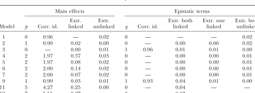
TABLE 6

Results from 100 simulations that each search over five 100-cM chromosomes with markers spaced every 10 cM

Main effects Epistatic terms

Extr. Extr. Extr. both Extr. one Extr. both

Model p Corr. id. linked unlinked q Corr. id. linked linked unlinked

1 0 0.96 — 0.02 0 — — — 0.02

2 1 0.99 0.02 0.00 0 — 0.00 0.00 0.02

3 0 — 0.00 0.01 1 0.96 0.01 0.01 0.00

4 2 1.97 0.37 0.03 0 — 0.00 0.00 0.01

5 2 1.97 0.08 0.02 0 — 0.00 0.00 0.01

6 2 2.00 0.14 0.02 0 — 0.00 0.00 0.01

7 2 2.00 0.07 0.02 0 — 0.00 0.00 0.01

9 1 0.99 0.03 0.01 1 0.93 0.04 0.01 0.00

11 5 4.27 0.25 0.00 0 — 0.04 — —

12 7 5.55 0.27 — 0 — 0.03 — —

TABLE 7

Results of the search over 12 100-cM chromosomes based on 100 simulations and the sample sizen⫽200

Main effects Epistatic terms

D Extr. Extr. Extr. both Extr. one Extr. both

Model (cM) p Corr. id. linked unlinked q Corr. id. linked linked unlinked

1 5 0 0.98 — 0.01 0 — — — 0.01

1 20 0 0.95 — 0.03 0 — — — 0.02

2 5 1 0.99 0.00 0.00 0 — 0.00 0.00 0.01

2 20 1 1.00 0.02 0.02 0 — 0.00 0.00 0.03

4 5 2 2.00 0.11 0.01 0 — 0.00 0.01 0.03

4 20 2 1.87 0.54 0.03 0 — 0.00 0.03 0.01

8 20 2 2.00 0.03 0.04 0 — 0.00 0.07 0.02

10 5 0 — 0.01 0.03 3 2.94 0.03 0 0.01

10 20 0 — 0.01 0.02 3 2.21 0.10 0.02 0.02

12 5 7 4.66 0.19 0.01 0 — 0.00 0.00 0.00

12 20 7 5.23 0.43 0.08 0 — 0.01 0.03 0.04

Dis the marker spacing,pis the true number of main effects,qis the true number of epistatic terms, Corr. id. denotes the average number of correctly identified terms, Extr. linked denotes the average number of extraneous terms that are linked to true QTL, and Extr. unlinked denotes the average number of extraneous terms that are not linked to true QTL.

particular cases (and a real analysis is always a particular In this article we did not address the problem of missing marker data. Currently in the QTL mapping case) when the forward selection procedure does not

detect the best model. Thus, although statistically we literature three methods exist, which are designed to solve this problem by using genotypes of neighboring do not expect much improvement by replacing forward

selection with a more refined search strategy, we still markers. They includeHaleyandKnott(1992) regres-sion, the E-M algorithm ofJansenandStam(1994), or recognize the need for further research in this direction.

Although this article is concerned solely with de- multiple imputations of missing genotypes proposed by Senand Churchill(2001) andBall (2001). We be-tecting main effects and pairwise interactions,

theoreti-cally the proposed method can be directly generalized lieve that the application of any of these methods will leave the mBIC unaffected by a moderate proportion to identify higher-order interactions. To retain control

over the type I error of the corresponding procedure, of missing marker data. The missing data methods can also be used to apply mBIC to search for QTL within it is anticipated that higher-order interactions should

be penalized even more than pairwise epistatic terms. intermarker intervals.

The method proposed in this article selects markers However, the utility of this approach needs to be verified

by additional research, since there are two main diffi- strongly associated with the trait and does not explicitly use the information from the distance between them. culties related to any extensions of our work. First is

the numerical complexity of the search over a rapidly Therefore, in principle the mBIC approach is not sensi-tive to map errors. However, the application of any of increasing number of models with higher-order

interac-tions, which can most likely be addressed by developing the missing data methods will make our method sensi-tive to map errors in the same way as standard interval a suitable search strategy and increasing computer

power. The second issue is more difficult and of a more mapping. Our method can be also influenced by selec-tive genotyping and genotyping errors, since selecselec-tive theoretical nature. If we do not have prior expectations

on the number of main and epistatic effects the method genotyping will change the correlation structure in the design matrix and might result in partial confounding outlined in this article can be used to control the overall

type I error. In this case, when we increase the potential of epistatic and main effects. However, our approach is able to select the proper markers out of many strongly number of regressors by including higher-order

interac-tions, we must also increase the penalties for main ef- correlated neighbors; therefore we believe that it is also robust to any partial confounding of main and epistatic fects and pairwise interactions. Thus, an attempt to

de-tect higher-order interactions will result in decreasing effects. The influence of genotyping errors will depend on the marker information that is affected. In our mBIC power of detection of simpler effects and can be offset

only by larger sample sizes. When some prior informa- criterion, as well as in other standard model selection criteria, the information on the data appears only in tion on the number of main effects and interactions is

available the power will be less affected since the method RSS. Thus, we do not expect a significant difference between our criterion and others with respect to the can be used in a subjective way via an appropriate

Foster, D. P., andE. I. George, 1994 The risk inflation criterion

Locating QTL, and more importantly their

interac-for multiple regression. Ann. Stat.22:1947–1975.

tions, remains an open problem in both the QTL map- _{George, E. I., andR. E. McCulloch, 1993 Variable selection via} ping and statistical communities. Current multiple in- Gibbs sampling. J. Am. Stat. Assoc.88:881–889.

Haley, C. S., andS. A. Knott, 1992 A simple regression method

terval mapping methods are plagued by two intimately

for mapping quantitative trait loci in line crosses using flanking

related issues. First is the problem of estimating the _{markers. Heredity69:315–324.}

number of QTL and their interactions. And second is Heath, S. C., 1997 Markov chain Monte Carlo segregation and linkage analysis for oligogenic models. Am. J. Hum. Genet.61:

the related issue of searching over the space of all

possi-748–760.

ble multidimensional models that comprise the compu- _{Jannink, J.-L., andR. Jansen, 2001 Mapping epistatic quantitative} tationally complex space. Realizing that the second issue trait loci with one-dimensional genome searches. Genetics157:

445–454.

is impacted by the approach of the first issue, we have

Jansen, R. C., 1993 Interval mapping of multiple quantitative trait

presented a model selection criterion that allows more _{loci. Genetics135:205–211.}

accurate assessment than the original BIC criterion, Jansen, R. C., andP. Stam, 1994 High resolution of quantitative traits into multiple loci via interval mapping. Genetics136:1447–

from which we started. Using simulations in a backcross

1455.

setting we demonstrate that the mBIC does well to locate

Kao, C.-H., Z-B. ZengandR. D. Teasdale, 1999 Multiple interval

multiple interacting QTL. Extensions of our method to mapping for quantitative trait loci. Genetics152:1203–1216.

Kilpikari, R., andM. J. Silanpa¨a¨, 2003 Bayesian analysis of

multilo-more general designs are possible and are currently

cus association in quantitative and qualitative traits. Genet.

Epide-under investigation. Furthermore, the proposed

crite-miol.25:122–135.

rion can be used outside the context of genetics to _{Lander, E. S., andD. Botstein, 1989 Mapping Mendelian factors}

underlying quantitative traits using RFLP linkage maps. Genetics

estimate the number of additive effects and interactions

121:185–199.

in the general framework of multiple regression.

Madigan, D., andA. E. Raftery, 1994 Model selection and account-ing for model uncertainty in graphical models usaccount-ing Occam’s We thank Jim Berger, Andreas Futschik, and Joanna Szyda for

window. J. Am. Stat. Assoc.89:1535–1546. helpful discussions and two anonymous reviewers for comments that

McQuarrie, A. D. R., andC.-L. Tsai, 1998 Regression and Time Series

greatly improved the presentation of the results. We also thank Adam

Model Selection. World Scientific Publishers, Singapore. Zagdanski and Monika Horobiowska-Kaczmarz for help in performing

Miller, A. J., 1990 Subset Selection in Regression. Chapman & Hall, simulations. The results reported in this article were presented at the

London. Seventh Purdue Symposium on Statistics, June 19–24, 2003. R.W.D.

Nakamichi, R., Y. UkaiandH. Kishino, 2001 Detection of closely is funded in part by grants from the U.S. Department of Agriculture- _{linked multiple quantitative trait loci using genetic algorithm.} Initiative for Future Food and Agricultural Systems (00-52100-9615) _{Genetics158:463–475.}

and the National Science Foundation (0115109-MCB). _{Piepho, H}.-P., andH. G. Gauch, Jr., 2001 Marker pair selection for mapping quantitative trait loci. Genetics157:433–444.

Raftery, A. E., D. Madigan and J. A. Hoeting, 1997 Bayesian model averaging for linear regression models. J. Am. Stat. Assoc.

LITERATURE CITED 92:179–191.

Satagopan, J. M., andB. S. Yandell, 1996 Estimating the number of

Akaike, H., 1974 A new look at the statistical model identification. _{quantitative trait loci via Bayesian model determination. Special} IEEE Trans. Automat. ControlAC-19:716–723.

Contributed Paper Session on Genetic Analysis of Quantitative

Balding, D.,A. D. Carothers, Y. L. Marchini, L. R. Cardon, A. _{Traits and Complex Diseases, Biometric Section, Joint Statistical} Vettaet al., 2002 Discussion on the meeting on statistical

mod-Meetings, Chicago. elling and analysis of genetic data. J. R. Stat. Soc. B64:737–775.

Satagopan, J. M., B. S. Yandell, M. A. NewtonandT. C. Osborn,

Ball, R., 2001 Bayesian methods for quantitative trait loci mapping

1996 Bayesian model determination for quantitative trait loci. based on model selection: approximate analysis using the

Bayes-Genetics144:805–816. ian information criterion. Genetics159:1351–1364.

Schwarz, G., 1978 Estimating the dimension of a model. Ann. Stat.

Boer, M. P., C. J. F. ter BraakandR. C. Jansen, 2002 A penalized

6:461–464. likelihood method for mapping epistatic quantitative trait loci

Sen, S., andG. A. Churchill, 2001 A statistical framework for quan-with one-dimensional genome searches. Genetics162:951–960.

titative trait mapping. Genetics159:371–387.

Bogdan, M., andR. W. Doerge, 2003 Mapping multiple interacting

Serfling, R., 1980 Approximation Theorems of Mathematical Statistics. quantitative trait loci with multidimensional genome searches.

Wiley, New York. Technical Report 04-03. Department of Statistics, Purdue

Univer-Siegmund, D., 2003 Model selection in irregular problems: applica-sity, West Lafayette, IN.

tions to mapping QTLs. Biometrika (in press).

Broman, K. W., andT. P. Speed, 2002 A model selection approach

Stephens, D. A., andR. D. Fisch, 1998 Bayesian analysis of quantita-for the identification of quantitative trait loci in experimental

tive trait locus data using reversible jump Markov chain Monte crosses. J. R. Stat. Soc. B64:641–656.

Carlo. Biometrics54:1334–1347.

Carlborg, O¨ ., L. AnderssonandB. Kinghorn, 2000 The use of

Silanpa¨a¨, M. J.,andE. Arjas,1998 Bayesian mapping of multiple a genetic algorithm for simultaneous mapping of multiple

inter-quantitative trait loci from incomplete inbred line cross data. acting quantitative trait loci. Genetics155:2003–2010.

Genetics148:1373–1388.

Churchill, G. A., andR. W. Doerge, 1994 Empirical threshold

Silanpa¨a¨, M. J., andJ. Corander, 2002 Model choice in gene map-values for quantitative trait mapping. Genetics138:963–971.

ping: what and why. Trends Genet.18:301–307.

Dempster, A. P., N. M. LairdandD. B. Rubin, 1977 Maximum

Uimari, P., andI. Hoeschele, 1997 Mapping linked quantitative likelihood from incomplete data via EM algorithm. J. R. Stat.

trait loci using Bayesian analysis and Markov chain Monte Carlo Soc. B39:1–38.

algorithms. Genetics146:735–743.

Fijneman, R. J. A., S. S. de Vries, R. C. JansenandP. Demant, 1996

Whittaker, J. C., R. ThompsonandP. M. Visscher, 1996 On the Complex interactions of new quantitative trait loci,Sluc1,Sluc2,

mapping of QTL by regression of phenotype on marker-type.

Sluc3, andSluc4, that influence the susceptibility to lung cancer

Heredity77:23–32. in the mouse. Nat. Genet.14:465–467.

Wolf, J. B., E. D. Brodie, III andM. J. Wade(Editors), 2000 Epistasis Fijneman, R. J. A., R. C. Jansen, M. A. Van der ValkandP. Demant,

and the Evolutionary Process. Oxford University Press, New York. 1998 High frequency of interactions between lung cancer

sus-Xu, S., 2003 Estimating polygenic effects using markers of the entire ceptibility genes in the mouse: mapping of Sluc5 to Sluc14.

Yi, N., andS. Xu, 2000 Bayesian mapping of quantitative trait loci _{Under the null hypothesis of no QTL 2 logL(Y|␪}ˆ_i)/

for complex binary traits. Genetics155:1391–1403.

L0(Y|␮ˆ ,␴ˆ) has asymptotically␹2distribution with 1 d.f.

Yi, N., andS. Xu, 2002 Mapping quantitative trait loci with epistatic

effects. Genet. Res.79:185–198. (Serfling 1980). Thus, P(S˜M_i⬎S˜0) is asymptotically

Yi, N., V. GeorgeandD. B. Allison, 2003a Stochastic search

vari-equivalent to

able selection for identifying multiple quantitative trait loci. Ge-netics164:1129–1138.

Yi, N., S. XuandD. B. Allison, 2003b Bayesian model choice and _2P

共

_Z⬎

√

_logn⫹_2(log(l⫺ _{1) or log(u}⫺ ₁₎₎

兲

_, search strategies for mapping interacting quantitative trait loci.

Genetics165:867–883.

whereZis aN(0, 1) random variable. Zeng, Z-B., 1993 Theoretical basis of separation of multiple linked

gene effects on mapping quantitative trait loci. Proc. Natl. Acad. Note that S˜1 ⬎ S˜0 if Equation A2 holds for at least

Sci. USA90:10972–10976.

one of the one-dimensional models. Therefore, by Bon-Zeng, Z-B., 1994 Precision mapping of quantitative trait loci.

Genet-ferroni inequality, for anyε⬎ 0 and sufficiently large

ics136:1457–1468.

nit holds

Communicating editor: J. B.Walsh

P(S˜1⬎S˜0)ⱕ2NmP

共

Z⬎

√

logn⫹2 log(l⫺1)

兲

APPENDIX: BOUND FOR THE TYPE I ERROR _⫹2NeP

共

_Z⬎

√

_{logn⫹2 log(u⫺1)}

兲

_⫹ε.

(A3) Our procedure recommends choosing the model that

maximizes the criterion

For eachx⬎0 it holds that

S˜(i)⫽log L(Y|␪ˆi)⫺

1

2(p(i)⫹q(i))logn _{P(Z ⬎x)ⱕ} 1

√

2␲e ⫺x2_/21

x.

⫺ p(i)log(l⫺1) ⫺q(i)log(u⫺1). (A1)

Thus (A3) yields The number of all possible one-dimensional models

[models for which p(i)⫹ q(i) ⫽ 1] is equal toNm⫹

P(S˜1⬎S˜0)ⱕ

2Nm

(l⫺1)√2␲n(logn⫹2 log(l⫺1))

Ne, where, as before,Nmis the number of available mark-ers andNe⫽(Nm(Nm⫺1))/2 is the number of possible

interactions. LetS˜1 denote the maximum of the crite- ⫹ 2Ne

(u⫺1)√2␲n(logn⫹2 log(u⫺1)) ⫹ε. rion (A1) over all such one-dimensional models and let

S˜0⫽logL0(Y|␮ˆ ,␴ˆ) be the value of the criterion for the

For the proposed valuesl⫽Nm/2.2 andu⫽Ne/2.2 the null model involving no markers (p⫹q⫽0). LetD⫽

right-hand side of the above inequality is approximately

p⫹qbe the number of terms in the model chosen by

equal to our procedure. It holds that

P(D⬎ 0)⫽P(S˜1 ⬎S˜0)⫹P(D⬎1,S˜1ⱕ S˜0). 4.4

√2␲n

冢

1

√logn⫹2 log(l⫺1)⫹

1

√logn⫹2 log(u⫺1)

冣

. We bound the probability of the first, dominating term

(A4) of the right-hand side of the above equality, under the

null hypothesis of no QTL.

Using the proposed values of l and u allows one to Consider a given one-dimensional model Mi and a

eliminate Nm and Ne from the bound numerator and corresponding value of our criterion

thus helps solve the multiple-comparisons problem. For the sample size n⫽ 200 andNm andNeused in

S˜Mi⫽logL(Y|␪ˆi)⫺

1

2logn⫺(log(l⫺1) or log(u⫺1)). our experiments the bound given by (A4) takes values from the interval between 0.0574 (for Nm ⫽ 252 and The modelMiwill be preferred over the model with no

Ne ⫽ 31,626; 12 100-cM chromosomes with markers QTL ifS˜M_i⬎S˜0, or equivalently

spaced every 5 cM) and 0.0801 (forNm⫽11 andNe⫽ 55; one 100-cM chromosome with markers spaced every 2 log L(Y|␪ˆi)

L0(Y|␮ˆ ,␴ˆ)

⬎log n⫹2(log(l⫺1) or log(u⫺1)) .