ABSTRACT
WINTON, COREY W. Parameter Estimation in Groundwater Models Using Proper Orthogonal Decomposition. (Under the direction of Dr. Carl T. Kelley.)
Parameter Estimation in Groundwater Models Using Proper Orthogonal Decomposition
by
Corey W. Winton
A dissertation submitted to the Graduate Faculty of North Carolina State University
in partial fulfillment of the requirements for the degree of
Doctor of Philosophy
Applied Mathematics
Raleigh, North Carolina 2012
APPROVED BY:
Dr. Pierre Gremaud Dr. Stacy Howington
Dr. Cass T. Miller Dr. Ralph Smith
DEDICATION
BIOGRAPHY
ACKNOWLEDGEMENTS
I cannot hope to thank everyone who has helped me achieve my degree. The following will attempt to thank, in some sort of chronological order, some of those who have made this possible.
• Obviously, I thank my parents Dennis and Rosemary Winton first. Without them none of this would be possible.
• Mrs. Fitzgerald and those involved with the SEEK program. Thank you for giving me an opportunity to learn and be challenged at an early age.
• Mr. and Mrs. Carrell and Betty Rainey and the many other teachers of Titusville area schools who challenged generations of students to reach for their goals and never settle for less than their absolute best. Thank you for preparing me so well for college, graduate school, and beyond.
• I cannot hope to list everyone from Asbury College who I want to thank, but want to mention Dr. Coulliette, Dr. Rietz, Dr. Charalambakis, Dr. Lee, and the rest of the Asbury mathematics department for encouraging me to pursue a career in mathematics.
• My fellow Asbury mathematicians, especially Skyler Speakman, Corey Robertson, Ben Flannery, Joel Kilty, and my math weekend teammates. I’m so thankful you all helped me finish my math degree from Asbury and inspired me to continue to graduate school.
• My fellow graduate students, especially Brendan O’Connor, Steve and Lindsay May, Ryan Siskind, and Teresa Selee. Thank you for helping me study, learn, and pass graduate exams, not to mention survive and enjoy graduate school to the fullest. • My team members and supervisors at ERDC in Vicksburg, especially Rob Wallace,
Dave Richards, Owen Eslinger, Amanda Hines, and Jeff Hensley. Thank you for helping me balance the pursuit of this degree and my job.
• Tim Kelley. It’s been an honor to learn from you and work with you the past years. I look forward to many productive years of collaboration ahead.
• My wife, Christy Paine Winton. Your encouragement and endurance through this process has been invaluable. Thank you for standing by me and encouraging me all the way through.
TABLE OF CONTENTS
List of Tables . . . ix
List of Figures . . . xi
Chapter 1 Introduction . . . 1
Chapter 2 Saturated Flow . . . 3
2.1 Model Development . . . 3
2.1.1 Introduction . . . 3
2.1.2 Derivation via Mass Conservation . . . 3
2.1.3 General Mass-Flux Equation . . . 5
2.1.4 Darcy’s Law . . . 8
2.1.5 Complete Single Phase Flow Equation for Steady State Domains . 10 Chapter 3 Single-Phase Groundwater Model . . . 11
3.1 2-D Model . . . 11
3.2 3-D Model . . . 12
3.3 Approximating the Hydraulic Conductivities . . . 13
3.4 Comparison to Data . . . 14
Chapter 4 Total Flux Boundary Condition . . . 15
4.1 Problem Statement . . . 15
4.1.1 Formulation . . . 15
4.1.2 Boundary Value Map . . . 17
Chapter 5 Proper Orthogonal Decomposition . . . 20
5.1 POD Background . . . 20
5.2 Classic Proper Orthogonal Decomposition . . . 21
5.3 POD For Saturated Groundwater Models . . . 22
5.3.1 The POD basis . . . 24
5.3.2 Sensitivity Calculation . . . 25
5.3.3 POD Reduced Model . . . 28
Chapter 6 Parameter Estimation . . . 29
6.1 Inverse Problems in Hydrogeology . . . 29
6.1.1 Approximating the Hydraulic Conductivities . . . 29
6.1.2 Optimization Methods . . . 30
6.2 Levenberg-Marquardt . . . 31
6.3 Optimization Algorithm . . . 32
6.3.2 Algorithm . . . 34
Chapter 7 Results . . . 37
7.1 2-D Results . . . 37
7.2 3-D Results . . . 43
7.2.1 Synthetic Column . . . 43
7.2.2 Laboratory Scale Synthetic Aquifer . . . 51
7.2.3 SPE10 . . . 59
Chapter 8 Inexact Levenberg Marquardt with Reduced Order Models. 62 8.1 Solving the Linear System . . . 62
8.1.1 Iterative Linear Methods . . . 63
8.2 Modifications to Optimization Algorithm . . . 64
8.3 Inexact Levenberg Marquardt with Reduced Order Models . . . 65
8.4 Tolerance Results . . . 66
8.4.1 Synthetic Column . . . 66
8.4.2 Noise: 0% . . . 67
8.4.3 Noise: 1% . . . 69
8.4.4 Noise: 5% . . . 71
8.4.5 Noise: 10% . . . 73
8.4.6 Parameter Values . . . 74
8.4.7 Laboratory Scale Synthetic Aquifer . . . 75
8.4.8 Noise: 0% . . . 75
8.4.9 Noise: 1% . . . 77
8.4.10 Noise: 5% . . . 79
8.4.11 Noise: 10% . . . 81
8.4.12 Parameter Values . . . 82
8.4.13 SPE10 . . . 83
8.5 Parameter Fit . . . 84
8.6 Results Discussion . . . 84
Chapter 9 Conclusions and Future Work . . . 86
References . . . 88
Appendices . . . 96
Appendix A Finite Element Method . . . 97
A.1 General Dirichlet BVP . . . 97
A.1.1 Equivalence of Forms . . . 98
A.2 General Neumann BVP . . . 99
A.3 Mixed and Inhomogeneous Boundary Conditions . . . 100
A.3.2 Inhomogeneous Boundary Conditions . . . 100
A.4 Discretization . . . 102
A.4.1 Linear Functionals . . . 103
A.4.2 Existence and Uniqueness . . . 103
A.4.3 Elliptic and Bounded . . . 105
A.4.4 Projection Theory . . . 107
A.4.5 The Galerkin Method . . . 108
Appendix B Functional Analysis . . . 110
B.1 Essential Functional Analysis Definitions . . . 110
Appendix C ADH . . . 114
C.1 POD with ADH . . . 114
C.2 Relevant Codes . . . 116
Appendix D PEST . . . 118
D.1 PEST - POD Interaction . . . 118
D.2 Variables . . . 118
D.2.1 General PEST Settings . . . 119
D.2.2 Levenberg-Marquardt Settings . . . 119
D.2.3 Output Settings . . . 121
Appendix E SCALAPACK . . . 122
E.1 Mesh Partition . . . 122
LIST OF TABLES
2.1 Key REV Characteristics . . . 5
7.1 Analysis for Column . . . 47
7.2 Relative Log-Transformed Parameter Error for Column . . . 48
7.3 Results for CSM Tank with Direct Solver . . . 54
7.4 Relative Log-Transformed Parameter Error for Tank . . . 56
7.5 Relative Log-Transformed Parameter Error for SPE10 . . . 59
7.6 SPE10 Results for 1e−6 Solver Tolerance . . . 60
8.1 Time (sec) for each ADH solution (serial) . . . 62
8.2 Analysis of Time (s) for Domain: HET, Noise: Data . . . 67
8.3 Analysis of Final Residual for Domain: HET, Noise: Data . . . 67
8.4 Analysis of Parameter Error for Domain: HET, Noise: Data . . . 68
8.5 Analysis of Model Calls for Domain: HET, Noise: Data . . . 68
8.6 Analysis of Time (s) for Domain: HET, Noise: 1 %. . . 69
8.7 Analysis of Final Residual for Domain: HET, Noise: 1 % . . . 69
8.8 Analysis of Parameter Error for Domain: HET, Noise: 1 % . . . 70
8.9 Analysis of Model Calls for Domain: HET, Noise: 1 % . . . 70
8.10 Analysis of Time (s) for Domain: HET, Noise: 5 % . . . 71
8.11 Analysis of Final Residual for Domain: HET, Noise: 5 % . . . 71
8.12 Analysis of Parameter Error for Domain: HET, Noise: 5 % . . . 72
8.13 Analysis of Model Calls for Domain: HET, Noise: 5 % . . . 72
8.14 Analysis of Time (s) for Domain: HET, Noise: 10 % . . . 73
8.15 Analysis of Final Residual for Domain: HET, Noise: 10 % . . . 73
8.16 Analysis of Parameter Error for Domain: HET, Noise: 10 % . . . 74
8.17 Analysis of Model Calls for Domain: HET, Noise: 10 % . . . 74
8.18 Conductivity Values for Column . . . 75
8.19 Analysis of Time (s) for Domain: ALL, Noise: Data . . . 75
8.20 Analysis of Final Residual for Domain: ALL, Noise: Data . . . 76
8.21 Analysis of Parameter Error for Domain: ALL, Noise: Data . . . 76
8.22 Analysis of Model Calls for Domain: ALL, Noise: Data . . . 76
8.23 Analysis of Time (s) for Domain: ALL, Noise: 1 % . . . 77
8.24 Analysis of Final Residual for Domain: ALL, Noise: 1 % . . . 77
8.25 Analysis of Parameter Error for Domain: ALL, Noise: 1 % . . . 78
8.26 Analysis of Model Calls for Domain: ALL, Noise: 1 % . . . 78
8.27 Analysis of Time (s) for Domain: ALL, Noise: 5 % . . . 79
8.28 Analysis of Final Residual for Domain: ALL, Noise: 5 % . . . 79
8.29 Analysis of Parameter Error for Domain: ALL, Noise: 5 % . . . 80
8.31 Analysis of Time (s) for Domain: ALL, Noise: 10 % . . . 81
8.32 Analysis of Final Residual for Domain: ALL, Noise: 10 % . . . 81
8.33 Analysis of Parameter Error for Domain: ALL, Noise: 10 % . . . 82
8.34 Analysis of Model Calls for Domain: ALL, Noise: 10 % . . . 82
8.35 Conductivity Values for Tank . . . 83
8.36 SPE10 Results . . . 83
8.37 Conductivity Values for SPE10 . . . 84
LIST OF FIGURES
2.1 Representative Elementary Volume . . . 4
2.2 Explanation of Darcy’s Experiment . . . 8
5.1 Distribution of Singular Values . . . 23
6.1 Optimization Algorithm for Full Model - Reduced Model - PEST Interaction 34 7.1 2-D Domain with Sensors . . . 38
7.2 “Data” Solution with 4x4 Conductivity Grid . . . 39
7.3 Initial Solution (Homogeneous Conductivity) . . . 40
7.4 Gauss-Newton Convergence from Homogeneous Initial Iterate . . . 41
7.5 Levenberg-Marquardt Iteration History . . . 42
7.6 Levenberg-Marquardt Solution . . . 43
7.7 Composition of Column . . . 44
7.8 Hydraulic Head of Column . . . 45
7.9 Location of Sensors . . . 46
7.10 Convergence of Optimizer for 0% noise . . . 49
7.11 Solutions of Column . . . 49
7.12 Solutions of Column With 10% Randomized Data . . . 50
7.13 Colorado School of Mines Tank . . . 51
7.14 Packing Method . . . 52
7.15 Allocation of Materials . . . 53
7.16 Location of Sensors in Tank . . . 53
7.17 Convergence of Optimizer for 0% noise on CSM Tank . . . 55
7.18 Exact Solution of Tank . . . 57
7.19 Solutions of Tank With 0% Noise . . . 57
7.20 Solutions of Tank With Measured Data . . . 58
7.21 Material Allocation for SPE10 . . . 59
7.22 Exact Solution of SPE10 . . . 60
7.23 SPE10 Solutions . . . 61
E.1 Partition of ScaLAPACK Matrix . . . 123
Chapter 1
Introduction
We describe an algorithm for model calibration of saturated flow codes using a reduced order model, specifically Proper Orthogonal Decomposition (POD). We will recover the hydraulic conductivity of materials in a domain from measurements of the hydraulic head and the pumping rates of any wells. We will use a nonlinear least squares approach to measure the quality of our approximation. We seek to minimize the sum of squared differences between data points and our simulated results by adjusting the values of hydraulic conductivity. We will develop models in both 2-D and 3-D and will demonstrate results for both. We measure the quality of our process by accuracy of the solution and computation time required to obtain that solution.
We begin our discussion with a brief outline of groundwater physics and equations. Our research extends only to saturated groundwater models and our discussion will be similarly limited. We will discuss the discretization of the groundwater equations for implementation in a finite element mesh. In Chapter 5, we discuss the implementation of Proper Orthogonal Decomposition (POD) in the optimization process. Our goal with POD is to reduce the number of full, expensive model calls necessary for the optimizer to find a minimizing solution. Chapter 6 describes the use of the Levenberg-Marquardt code PEST to find a suitable suite of parameters to match data. Chapter 7 will detail the results we have found by using POD in saturated groundwater models. In Chapter 8, we explore how inaccuracies in the linear solver affect the solution speed and quality.
Chapter 2
Saturated Flow
2.1
Model Development
2.1.1
Introduction
Our research focuses on parameter estimation in porous media with a single liquid phase. In this chapter, we will derive the equations that govern steady-state, saturated flow through an immobile (or non-deformable) porous medium. We are careful to note the methods described later in this document hold only under these conditions. For the sake of clarity, vectors will be represented in italicized boldface (v) and matrices or tensors will be represented in bold (M).
2.1.2
Derivation via Mass Conservation
Figure 2.1: Representative Elementary Volume
In this work, we deal strictly with single phase flow in a saturated medium but for the sake of completeness in the derivation we will note other phases with the notationα, where α=s, l,org for solid, liquid, or gas, respectively. The void space (also called the pore space) is represented withα =p.Distinct species present in each phase–for instance multiple gases–are represented with the superscript i.
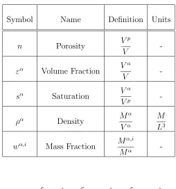
Table 2.1 describes several characteristics for our REV.
We can balance several of these properties over the volume. We see
X
α
εα = 1 : Volume Fractions sum to 1,
X
i
wα,i = 1 : Mass Fractions within each phase sum to 1,
X
α6=s
sα = 1 : Saturation of non-solid phases sum to 1.
We use mass-averaged velocity in our calculations so that macroscale properties are directly related to conservation principles. That is,
vα =
R
Ωvαρα dr
R
Ωρα dr
Table 2.1: Key REV Characteristics
Symbol Name Definition Units
n Porosity V
p
V
-εα Volume Fraction V α
V
-sα Saturation V
α
Vp
-ρα Density M
α
Vα
M L3
wα,i Mass Fraction M α,i
Mα
-and we see
ραvα =
R
Ωρα dr
R
Ω dr ×
R
Ωvαραdr
R
Ωρα dr =
R
Ωvαρα dr
R
Ω dr
.
2.1.3
General Mass-Flux Equation
We have established our properties across the REV and turn to conservation of mass to develop our model [77], [51]:
[Change In Mass Rate] = [Mass Inflow Rate] - [Mass Outflow Rate] , (2.2)
or
[Accumulation of Mass] = [Net Advective Transport (Flow)] + [Non-Advective Transport]
+ [Reactions] + [Interphase Mass Exchange] + [Sources].
(2.3)
value problem, following the derivation in [70]. We first describe accumulation of mass, the change over time of a species i in phaseα over volume V:
Accumulation of Mass =V ∂ ∂t ε
αραwα,i
. (2.4)
We next turn our attention to Net Advective Transport (Flow). We examine flow through a sample cubic volume with vertices at x, x+ ∆x, y, y+ ∆y, z, z+ ∆z. We define vα
x as
the mass-averaged velocity of theα-phase in the positivex-direction andAyz = ∆y∆z as
the area of the face where x is fixed. Total mass of the i species in the α phase passing through that face into the volume V is given by
Mxα,i= Ayzεα ρα vxα w α,i
x. (2.5)
Similarly, total mass passing through the opposite face, out of the volume is given by
Mxα,i+∆x = Ayzεαραvxαw α,i
x+∆x. (2.6)
We expand (2.6) with a Taylor’s series at the initial face and keep only the first order terms to see
Mxα,i+∆x = Ayzεα ρα vxα w
α,i+εαραwα,i∆x∂vxα
∂x x . (2.7)
Over our REV, we assume porosity (ε), density (ρ), and mass fraction (w) are constant and need only expand velocity in (2.7). Thus, net advective transport of the ispecies in the α phase in the x-direction is given by
Mxα i−Mxα i+∆x = −εαραwα i∆x∂v
α x ∂x x . (2.8)
We apply (2.8) to the x, y and z directions, recall that ∆x×∆y×∆z =V and see
Net Advective Transport =−V∇ · εαραwα ivα. (2.9) We will characterize non-advective transport of theispecies in the α phase for a volume
present in all terms, we factor it away and have the general mass balance equation:
∂ ∂t ε
αραwα,i
=−∇ · εαραwα,ivα+jα,i
+ (ψα,i+Rα,i+Sα,i). (2.10)
We sum (2.10) over all species and note several terms can be simplified:
• Change in mass due to phase change across each species i is the total change in mass for each phase α:
X
i
ψα,i =ψα.
• Change in mass due to sources/sinks across each species i is the total change in mass for each phase α:
X
i
Sα,i =Sα.
• Mass-fractions (wα,i) for each species i in phaseα sum to 1:
X
i
wα,i = 1.
Conservation of mass allows us to eliminate some terms:
• Total change of mass across all species due to reactions is zero:
X
i
Rα,i= 0.
• Sum of non-advective flux across all species within a single phase is zero:
X
i
jα,i= 0.
We only investigate movement of a single fluid phase in the following research, so we eliminate the phase-change termψα and drop the superscript α for all other terms. This leaves our general equation for accumulation of mass of a single phase:
∂
We turn to Darcy’s Law to describe the velocity of the liquid in our domain. As we describe the fluid moving through the solid domain, we assume the solid is immovable and has no velocity component.
2.1.4
Darcy’s Law
Henry Darcy, a civil engineer in Dijon, France, motivated by the concern over public water supply was driven to investigate better designs for water purification through filtered sands. This led him “to determine the laws of flow of water through sand” [32] and his initial results were published in 1856. Darcy constructed an apparatus similar to the one shown in Figure 2.2 [12]. The volumetric flow rate Q (units: L3/T) was
Figure 2.2: Explanation of Darcy’s Experiment
expressed ∂h/∂l. His calculations gave rise to Darcy’s Law:
Q
A =q =
−k(h1−h2)
l =−k ∂h
∂l. (2.12)
The proportionality constantk(L/T) represents the hydraulic conductivity of the medium. This value represents the ease or difficulty a fluid has passing through a porous medium. The minus sign conveys that flow occurs in the direction of decreased head in the manome-ters. For clarification, (2.12) can be stated as:
Rate of flow through a cross sectional area is proportional to hydraulic gradient. (2.13) This result is only valid for 1-D flow. To generalize the results for 3-D flow, we describe an anisotropic material with the conductivity tensor K. The i, j coefficient entry of K describes flow in the i direction in response to a unit gradient in the −j direction.
qx = −Kxx
∂h
∂x −Kxy ∂h
∂y −Kxz ∂h ∂z,
qy = −Kyx
∂h
∂x −Kyy ∂h
∂y −Kyz ∂h ∂z,
qz = −Kzx
∂h
∂x −Kzy ∂h
∂y −Kzz ∂h ∂z
and Darcy’s Law for 3-dimensions is given by:
q =−K· ∇h.
In our examples, we do not have anisotropic materials. Instead, the flow response for any given gradient is only along the lines of that gradient and is uniform in all direc-tions. Therefore, for any material the conductivity tensor can be replaced with a single coefficient κ. We note the flux of a liquid is equivalent to the volume fraction (ε) of that phase times the velocity. We see the Darcy flux can be represented
In later discussions, this isotropy is very important as it allows us to characterize the hydraulic conductivity throughout the domain as a piecewise constant function where each material has a single scalar conductivity value, not a tensor. This, along with the linearity of the differential equation, allows us to recombine the matrix and vector as shown in (3.13).
2.1.5
Complete Single Phase Flow Equation for Steady State
Domains
We substitute (2.14) in (2.11) and have:
∂
∂t(ερ) =−∇ ·(−κ ρ∇h) +S. (2.15)
In the following examples, we will only examine steady state problems (∂t∂(ερ) ≡ 0). While field systems are rarely at steady state, for conditions in which boundary conditions and sources and sinks are invariant with time, heads will tend toward a steady value with increasing time. We will assume steady state conditions in this work, but the methods to be explored can be expended to the transient case.
These assumptions give us the following equation for the hydraulic head (h) of a fluid in an isotropic, single fluid domain given a source termS, hydraulic conductivity κ, and density ρ:
−∇ ·(κρ∇h) =S.
We assume that spatial gradients in density of our fluid are small in comparison to gradients in head of the fluid and conductivity of the materials. Therefore, we assume ρ
is constant and our final equation is:
Chapter 3
Single-Phase Groundwater Model
We apply our method to both 2-D and 3-D domains. The 2-D domain serves only as a proof-of-concept and is on a small scale to be run easily withinMatlab. The parameters in the 2-D example serve only to test our algorithm; they are not representative of actual data or scenarios.
Our 3-D examples are a mix of simulations and actual data. When we use simulated domains, the scale of the domain is intended to represent possible “real-world” scenarios and all values approximate those we would experience (with the assumptions previously described) in field tests.
3.1
2-D Model
−∇ ·(κ(x, y)∇h(x, y)) = g(x, y) (3.1)
h(0, y) = h0 (3.2)
h(1, y) = h1 (3.3)
∂h
∂n(x,0) = 0 (3.4)
∂h
∂n(x,1) = 0. (3.5)
We leth0 =.4km, h1 = 1km. The conductivities of the sixteen equally spaced, isotropic materials are in the range κ(x, y)∈ [10−10,10−2]. We place two wells g(x, y) that pump at a rate of ≈6×10⁻² m3/s. These parameters are designed solely as a proof-of-concept for our method and do not represent any real-world example.
To generate the hydraulic head h(x, y), we use the finite element implementation coded by [38] to discretize and solve (3.1)-(3.5) with
Ah =f. (3.6)
3.2
3-D Model
Our 3-D examples are also saturated and in steady-state. The materials are all isotropic and we still have only a single fluid phase. Unlike the 2-D example, we do not include any wells. That is, g(x) ≡ 0 from (3.1). To ensure that the hydraulic head h are uniquely defined by material conductivities κ, we must introduce a flow boundary condition. The total flux boundary condition is stated here in (3.7c). The derivation and need for this boundary condition is given in (§4). Our system is
−∇ ·(κ(x)∇h(x)) = 0 (3.7a)
h(x) = α on ΓD (3.7b)
Z
ΓQ
where
x ∈Ω⊂R3, (3.8a)
h ∈RN, (3.8b)
∂Ω = ΓD∪ΓQ, (3.8c)
ΓD∩ΓQ = Ø. (3.8d)
To discretize and solve our 3-D model, we use ADH, developed at the United States Army Corps of Engineers (USACE) lab in Vicksburg, MS. In Appendix C, we discuss what steps were taken to extract the necessary information and the relevant model set-tings we use. Just as in the 2-D example (albeit with significantly more complexity in 3-D), we build the matrix A and vector f to solve
Ah =f.
3.3
Approximating the Hydraulic Conductivities
We represent the conductivity field as a piecewise constant function. In our discussion of the optimization process (§6) we investigate how this representation of the conductiv-ities affects our solution. We let χi(x) be a characteristic function that indicates where
material i (and therefore hydraulic conductivity κi) appears in the domain and depict
the hydraulic conductivity in the domain as
κ(x) = X
i
κiχi(x) (3.9a)
X
i
χi(x) = 1. (3.9b)
In both the 2-D and 3-D examples, we use finite elements to discretize the weak form of the system of equations. Appendix A describes how the finite element method achieves this task. In general, we multiply the flow equation by a test function v, integrate, and, using Green’s identity, reach the weak form of the flow equation:
Z
Ω
κ(x)∇h(x)∇v(x)dx =
Z
Ω
The discretized form of (3.10) is represented as a linear system
Ah =f.
The isotropic, piecewise constant conductivity function allows us to separate the single operator A, f into an operator on each material, seen by substituting (3.9) into (3.10):
X
i
Z
Ω
χi(x)κi∇h(x)∇v(x)dx =
Z
Ω
f(x)v(x)dx. (3.11)
We let
Ai =
R
Ωχi(x)∇h(x)∇v(x)dx (3.12) Dirichlet boundary conditions are implemented by directly changing the stiffness matrix A. Those changes are contained in A0. In Appendix C, we describe the construction of each sub vectorfi. So, our matrix and vector can be described:
A = A0+
X
i
Aiκi (3.13a)
f = f0+X
i
fiκi. (3.13b)
3.4
Comparison to Data
The purpose of the methods described in later chapters of this document is to find a set of hydraulic conductivities that best fit provided hydraulic head data. The residual vector R contains the difference between the model approximation of hydraulic head h
given hydraulic conductivity κ and data d for M points is
R(κ)i =hi−di, i= 1, ..., M. (3.14)
Our methods will minimize the least-squares error: 1
2min||R(κ)|| 2 2 =
1
2min R(κ)
TR(κ)
Chapter 4
Total Flux Boundary Condition
In this chapter, we discuss the formulation, construction, and solution of the “Total Flux” boundary used in 3.7c. The experimental data that we wish to compare to consists of a set of heads over a heterogeneous domain in which a known quantity of fluid flows across one boundary and a Dirichlet condition is maintained at the opposite face with no flow conditions on the other four boundaries. The ideas are similar in two dimensions with two no flow boundaries. The flux boundary is specified in integral form as the total flux over the face, or edge in two dimensions, of the domain. An additional constraint is that the head is constant, but unknown, across the flux boundary.
Because this flux boundary condition is not known everywhere on the domain as with typical second-kind boundary conditions, it is necessary to derive the appropri-ate boundary conditions in a non-standard manner. Conceptually, we seek a constant Dirichlet boundary condition such that the specified integral flux condition is met. The linearity of the problem makes this a straightforward calculation.
4.1
Problem Statement
4.1.1
Formulation
We develop a strategy to solve the BVP in a domain that has mixed boundary conditions. We consider
where x is considered in the domain Ω with boundary ∂Ω. The boundary has a mix of three non overlapping boundary conditions, Dirichlet (D), Neumann (N), and Flux (Q). So
x ∈Ω⊂R3, (4.2)
h ∈RN, (4.3)
∂Ω = ΓD ∪ΓN ∪ΓQ, (4.4)
ΓD ∩ΓN ∩ΓQ = Ø. (4.5)
In general, there may be several boundary conditions of each type
ΓD = Γd1 ∪...∪ΓdN d, (4.6a)
ΓN = Γn1 ∪...∪ΓnN n, (4.6b)
ΓQ= Γq1 ∪...∪ΓqN q. (4.6c)
Each type of boundary condition will be represented as shown below:
Γdi ⇒ h(x) =αdi, x ∈Γdi, (4.7a)
Γni ⇒
∂h(x)
∂n =βni, x ∈Γni, (4.7b)
Γqi ⇒
R
Γqi(κ(x)∇h(x))·n dS =φqi, x ∈Γqi. (4.7c)
The solution to (4.1) is given by
h =hDN +
X
N q
γihqi ∈R
N
, (4.8)
where hDN and hqi are solutions to (4.1) with boundary conditions modified as follows:
on ΓQ:
∇ ·(κ(x)∇h(x)) = f(x)
Γdi ⇒ h(x) =αdi, x ∈Γdi,
Γni ⇒
∂h(x)
∂n =βni, x ∈Γni,
Γqi ⇒ h(x) = 0
• To compute hqi, we set h = 0 on ΓD,
∂h
∂n = 0 on ΓN, and h = 1 on ΓQ:
∇ ·(κ(x)∇h(x)) = f(x) Γdi ⇒ h(x) = 0,
Γni ⇒
∂h(x)
∂n = 0,
Γqi ⇒ h(x) = 1
We fix γi to satisfy the flux boundary condition on each relevant boundary. The flux
through each boundary Γqj is given by
Z
Γqj
(κ(x)∇hDN(x))·n dS+ Nq X i=1 γi Z Γqj
(κ(x)∇hqi(x))·n dS =φqj, j = 1...Nq, (4.9)
and these Nq equations provide the relationship for γi.
4.1.2
Boundary Value Map
The following discusses how we compute the flux for the boundary condition in (4.7c). For sake of clarity, the examples will be done in 1-D but can be expanded to 2-D and 3-D domains.
To calculate the boundary flux terms
Z
Γqj
κ(x)∇h∗(x)dS
!
, we turn to the deriva-tion in [4]. For all pointsx∈[0, `], we represent the flux at that point with
σ(x) = −κ(x)dh(x)
dx . (4.10)
conserved through the boundaries. That is, all mass passes through a boundary or is accounted for by an internal source of flux g(x). Over a 1-D domain x ∈ [0, `], the conservation of flux demands
σ(`) +σ(0) =
Z `
0
g(x)dx. (4.11)
At the boundaries of the domain, we denote the flux σ0, σ`. If we take any arbitrarily
small slice of the domain x∈[0, a], flux is conserved on that segment if
σ(a) +σ0 =
Z a
0
g(x)dx.
As we take a → 0, we can see that σ(0) = σ0. Similarly, we can show σ(`) = σ`, where
σ` is the prescribed flux through the right hand boundary. Thus,
σ`+σ0 =
Z `
0
g(x)dx.
Construction of Map
We construct a method that will explicitly compute the fluxσ0, σ`through each Dirichlet
boundary using information constructed by the full model simulator. This can be done with the information normally discarded in the finite element formulation of the load matrix.
For the sake of clarity, we return to a simple 1-D domain and use linear shape functions
u. Each element e is bounded by two nodes and, locally, we can represent the equations as
ae11ue1+ae12u2e =f1e+σ(se1), ae21ue1+ae22u2e =f2e−σ(se2),
a1
11u1 + a112u2 = f11 + σ(0)
a121u1 + (a221 +a211)u2 + a212u3 = f21+f12 − σ(x −
1) +σ(x+1)
a221u2 + a222u3 = f22 − σ(x − 2)
We represent the jump in flux at each node with [[σ(xi)]] = ˆfi, where ˆfi is zero except
in the case of a prescribed source. We see that the vector contains all of the boundary flux information, as well as any interior sources.
For Dirichlet nodes, the information in the matrix is replaced by a one on the diagonal and zero elsewhere in the corresponding row. Similarly, the vector entry that corresponds to a Dirichlet node is replaced with the prescribed Dirichlet boundary value. This dis-carded information provides the necessary equations to ascertain the flux through a given boundary.
For example, in the 1-D case, the entries in the matrix and vector for a Dirichlet node would be
A11u1+A12u2 = F1+σ(0), (4.12a)
AN,N1uN−1+AN NuN = FN −σ(`). (4.12b)
We store this information separately. After we have solved the system of equations to yield u1, u2, uN−1, uN, we return to (4.12) to obtain σ(0), σ(`). We note (4.12) can be
extended to the 2-D and 3-D cases by maintaining the corresponding matrix / vector structure and equations for the boundary nodes.
Once we have solved for each of the sub-solutions in (4.8), the flux value on any boundary Γqj is given by
Z
Γqj
κ(x)∇h∗(x)dS
!
=Xσh∗(xk), xk ∈Γqj, (4.13)
Chapter 5
Proper Orthogonal Decomposition
Proper Orthogonal Decomposition (POD) is one way to construct a reduced order model. The purpose of such models is to replace an expensive simulation within an optimization loop with a surrogate that is inexpensive to evaluate but still accurate enough to improve the fit to data. A typical approach [11] is to perform an optimization based on the surrogate and then evaluate the expensive simulation one or more times, both to decide whether or not to terminate the optimization and to update the surrogate for the next pass through the optimization loop.
5.1
POD Background
POD is a classical approach with roots in the control of fluids [50, 60, 63, 41]. POD has been developed using several different techniques. The earliest development of POD was under the name “Principal Component Analysis” (PCA) by Karl Pearson in 1901[74]. Using a different technique, Kari Karhunen and Michel Lo´eve developed the Karhunen-Lo´eve Decomposition (KLD) in 1955 [61]. Another method of performing POD is through use of the Singular Value Decomposition (SVD). The SVD was first introduced in 1873 and 1874 by Eugenio Beltrami [6, 10] and Camille Jordan [48, 49]. An excellent review of the early history of the SVD is given by [82]. The current method of calculating the SVD was presented by Gene Golub and William Kahan [39]. The three techniques for deriving the POD are shown to be equivalent in [59].
assuming knowledge of the conductivity tensor, use that model as a predictive tool. One can also use the POD projection to construct useful preconditioners [64]. Control applications have been reported in [85, 14, 63, 62, 3, 57]. POD has frequently been used as a reduced order model in turbulent flows [18, 7].
POD is a surrogate for the simulator that uses the simulator’s own discretizations and physics models. The advantages of POD over approaches that model the objective function φ
φ(κ) = 1
2kR(κ)k 2
, (5.1)
such as neural networks or interpolatory models [76, 20, 78, 43], is that POD directly uses the finite element discretization in hand and can exploit the least-squares structure via simple projections. The disadvantage is that, as with the sensitivity equations ap-proach to computing the Jacobian, one must modify the finite element code to extract information. We have done that with the ADHsimulator.
5.2
Classic Proper Orthogonal Decomposition
In the applications of POD listed above, one begins with a set of snapshots. Snapshots are solutions of the PDE corresponding to an array of parameter values and evaluated at various times of the solution evolution [13]. There is currently no rigorous method for constructing the set of snapshots [42]. However, it is very important that the full solution can be well approximated in the span of the snapshot set [13]. If an aspect of the true solution is not contained in the snapshot set, it cannot be approximated by the POD model.
There will be much redundant information contained in the snapshot set. It is typical to use the SVD [68, 27, 59] to reduce the basis and obtain a set of basis vectors that contain most of the relevant information in the snapshot set. The following shows how to approximate the error present in a truncated POD basis.
Error in POD Projection We start with the set of n snapshot vectors si, i = 1...n
where each si ∈RN and form the matrix
The SVD of that matrix is
S=UΣVT,
where Σ is a diagonal matrix with entries Σ = diag(σ1, ..., σn), σ1 ≥ σ2 ≥ ...≥ σn ≥0.
U, the left hand singular matrix, is an orthogonal matrix with the same range as S. V holds the right hand singular vectors.
The POD basis is formed from the d eigenvectors in Ucorresponding to the largest
d eigenvalues. To determined, we note the following error approximation algorithm. Let PUsi be the projection of the snapshot si onto the span of the POD basis from
U. The error of this approximation can be given by
εi =|si −PUsi|
2
.
The total error for the approximations of each snapshot is given by the sum of the discarded eigenvalues
ε =
n
X
i=1
εi = n
X
i=1
|si−PUsi|2.
As shown in [42, 59, 56] and others, this error can also be represented
ε=
n
X
i=d+1
σi2.
Therefore, to find a basis with approximation error less than some prescribed errorδ, we must find the smallestd such that
Pd
i=1σ 2
i
Pn
i=1σ2i
≥1−δ.
As shown in [42, 13, 17] and others, one normally choosesδ ≥.9, signifying the reduced basis is able to capture 90% of the physics contained in the snapshot set.
5.3
POD For Saturated Groundwater Models
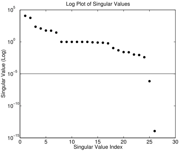
0 5 10 15 20 25 30 10−15
10−10 10−5 100 105
Singular Value Index
Singular Value (Log)
Log Plot of Singular Values
Figure 5.1: Distribution of Singular Values
vectors of that solution to the parameters as a basis. We scale the basis by solving the solution and sensitivities with log transfomed conductivities [15]. For our application, we utilize the total flux boundary condition described in §4. As such, we will have at least two sub-solutions and the sensitivities of those sub solutions in the basis.
5.3.1
The POD basis
The following will discuss the calculation of the 2N + 2 POD basis. We use the sub-solutions of (4.8) and their sensitivities to the K material parameters (5.5) to form
B=span hDN,{∂hDN/∂κk}Kk=1,hQ,{∂hQ/∂κk}Kk=1
. (5.2)
Unlike the use of POD for time-dependent problems, we need not create a basis by applying a singular value decomposition to a sequence of “snapshots”. Instead, we apply the singular value decomposition to this basis B and keep only those singular vectors that correspond to singular values greater than 10−5. The orthonormal basis for the significant singular vectors of B are stored in the columns of U.
Basis Expansion
As we perform the optimization algorithm described in §8, we do not discard the basis information from one iteration to the next. Instead, the new vectors of (5.2) are added to the previous basis and the entire system is orthogonalized. Vectors corresponding to small singular vectors are discarded and the new, expanded basis is used in the optimization routine.
By reusing the previous basis information, the reduced order model becomes more accurate as we iterate and the basis becomes more robust. We note that additional basis vectors increase the dimension of our reduced order model. Our parallel implementation of the SVD (Appendix E) ensures that even for bases with ≈ 100 vectors, the reduced order model is significantly faster than the full model.
Sensitivity Scaling
A basis consisting of solutions and sensitivities must be appropriately scaled, otherwise, a singular value decomposition will arbitrarily return small singular values [15]. Our calcu-lation of the sensitivities is scaled by solving against the log-transformed conductivities. That is,
κk =epk,
∂κk
∂pk
and our basis (5.2) is
B=span hDN,{∂hDN/∂pk}Kk=1,hQ,{∂hQ/∂pk}Kk=1
. (5.3)
We note the vector norm for the log-transformed sensitivities are within an order of magnitude of one another. Also, each sensitivity vector is within two orders of magnitude of the solution vector. Due to the relative similarity in norm, we are assured the SVD will not discard information from poor scaling.
5.3.2
Sensitivity Calculation
We are able to compute the sensitivity of the solution to the K material parameters without significant additional computational effort. We recall the solution to our BVP is given by (4.8) and shown again here:
h =hDN + Nq
X
i=1
γihqi ∈R
N, (5.4)
We differentiate with respect to the log-transformed parameterspk to see the sensitivities
are
∂h
∂pk
= ∂hDN
∂κk ∂κk ∂pk + Nq X i=1 γi
∂hqi
∂κk
∂κk
∂pk
+ ∂γi
∂κk
∂κk
∂pk
hqi
, (5.5)
or
∂h
∂pk
=epk · ∂hDN
∂κk + Nq X i=1
γiepk ·
∂hqi
∂κk
+epk · ∂γi
∂κk
hqi
. (5.6)
Flux Coefficient Sensitivities To compute ∂γj
∂κk
, we analyze the response each of the Nq equations that satisfy the flux
boundary condition (4.9) (shown again here) against the K material propertiesκk:
Z
Γqj
(κ(x)∇hDN(x))·n dS+ Nq X i=1 γi Z Γqj
to yield (5.8). Recall from§2 that we use zonation to represent the material conductivity field. Thus,
κ(x) = P
kκkχk(x)
∂κ(x)
∂κk
= χk(x)
Also, the flux through the boundary is set as a boundary condition and does not respond to perturbations in the material parameters:
∂φqj
∂κk
≡0.
Finally, we note the flux map in §4 can be applied to any vector in the solution space. That is, we can apply our technique to
Z
Γqj
(κ(x)∇h∗(x))·n dS
as well as to
Z
Γqj
κ(x)∇∂h∗(x)
∂κk
·n dS.
The system of equations that must be solved for ∂γj
∂pk
is given by:
∂ ∂pk
R
Γqj(κ(x)∇hDN(x))·n dS
+ PNq
i=1
γi∂p∂k
R
Γqj(κ(x)∇hqi(x))·n dS
+ ∂p∂γ
k
R
Γqj(κ(x)∇hqi(x))·n dS
= 0,
for j = 1...Nq.
We solve this system for ∂γj
∂pk
for each j = 1...Nq. It is noted that Nq is very small and
Solution Sensitivities We compute ∂h∗
∂pk
analytically (whereh∗ represents bothhDN and all solutionshqj). We
do this by exploiting zonation and the linearity of the problem. We note that all work done to precondition and factor the matrix in the original solve need not be redone for the sensitivity computation. We reuse the same matrix factorization, thus adding very little computational effort to the process.
The finite element discretization of (4.1) for any of the boundary conditions in (4.7) will yield
Ah∗ =f∗. (5.8)
We note the structure and values inA(κ) are not changed, regardless of the values on the boundary. We are not manipulating the structure of the problem when we solveh∗, only the value of the boundary conditions. The boundary condition information is contained in f∗. Appendix C describes the derivation of the terms in (5.8) and how the boundary information affects f∗.
As previously described, we can represent the matrixAand each vectorf∗ as a linear combination of sub matrices and vectors:
A = A0+PkAkκk (5.9a)
f∗(κ) = f∗0+P
kfkκk. (5.9b)
Again, we note that the information for the boundaries is contained in f∗0, each fk
is constant. A0 contains the information for the Dirichlet nodes and contains only the entries 1 and 0 on the diagonal, depending on whether the corresponding node is con-strained by a Dirichlet boundary condition. Similarly, the entries in f∗0 hold the values at those nodes.
We calculate the sensitivity of each solutionh∗ to the parametersκk by differentiating
(5.8) and substituting the information from (5.9).
A∂h∗
∂κk
=fk−Akh∗. (5.10)
5.3.3
POD Reduced Model
With coefficient and sub-solution sensitivities, we form the POD basis B. We orthogo-nalize the basis with an SVD and keep only those d vectors corresponding to singular values of magnitude greater than 10−5. Those orthogonal vectors are stored as the new basis U ∈RN×d. We let W ∈
RN×d be an orthonormal basis for AU. The reduced order
model for each sub-solution is
WTA0U u`+
X
i
κiWTAiU u` =WTf
{`} 0 +
X
i
κiWTfi, `=DN, qi
or
WTAUu` =WTf{`}, (5.11)
where
WTAU ∈ Rd×d,
WTf{`} ∈
Rd,
and the sub-matrices Ai are calculated as previously discussed. We note d << N and
the effort to solve this d×d system is significantly less than required to solve the full model.
The reduced model solution for hydraulic head is compared to data via
h` =Uu`, `=DN, qi
and
h =U uDN + Nq
X
i
γiuqi
!
. (5.12)
The residual that we will minimize is our approximation of hydraulic head h against the M data points di
Chapter 6
Parameter Estimation
6.1
Inverse Problems in Hydrogeology
We will approximate the material parameters by applying a Levenberg Marquardt op-timization code to a reduced order model generated through Proper Orthogonal De-composition. Ours is not the only approach to solve nor model the inverse problem for groundwater problems. The survey of [67] categorizes methods by how the authors parameterize the domain, how they model the forward problem, and which optimiza-tion scheme is used to fit the parameters. Their conclusion is that the various inverse methods — including those similar to our approach — all have merit but some are more appropriate than others for a sample problem. They conclude a blocked approach to parameterization such as ours is convenient for domains in which the boundaries are distinct. In the following, we survey other approaches to construction and optimization of the minimization problem.
6.1.1
Approximating the Hydraulic Conductivities
will not faithfully represent flux. The authors in [5] recommend blocks at least one tenth the size of the full domain.
Alternatively, one could parameterize the model with many small homogenous zones. If more zones than data points are used, the system is under-determined and no unique solution will exist. One can employ a regularization technique to move toward conver-gence to a unique solution. In [84], the authors apply both Tikhonov regularization [83, 87] and a singular value decomposition to approximate the material properties in an under-determined system. In [71], an analysis of cost of these regularization schemes is performed.
Both of the previous approaches create or assume some zones of uniform conductivity. In [30] the authors describe the construction and limitations of the “zonation” approach. They note that pilot points allow the modeler to avoid constructing the zones independent of the optimization process. Instead, as part of the parameter estimation process the location of the materials changes. In [55], the authors seek to discern which not only best fit of parameters, but also how many parameters to optimize. They provide an algorithm by which the complexity of the model is considered along with the fit to data of the end result.
Our depiction of the conductivity field is in the form of a small number of homogenous material zones. While we do not adjust the zone locations in the course of our optimiza-tion nor do we adjust the number of zones present, our method could be included during the parameter fitting phase of both of those techniques.
6.1.2
Optimization Methods
We construct a reduced order model with Proper Orthogonal Decomposition, then use a Levenberg-Marquardt [58, 65, 72, 28, 52] (LM) code PEST [31] to optimize parameters in that model. As noted in [45] and others, LM is widely used, but requires a large number of function calls to be effective. They use the adjoint state method to compute the derivatives of the objective function. Their approach allows them to compute the jacobian matrix for an LM method at a cost independent of the number of parameters. The construction of our reduced order model allows us to compute an analytic jacobian with very little computational effort. As noted in [91], the computation and accuracy of the jacobian vectors drive the success of the inverse problem.
have approached the problem with stochastically and sample posterior distributions of pa-rameters [40, 90]. Markov chain Monte Carlo (McMC) methods are a popular stochastic approach to the optimization method [36]. McMC methods determine the next iteration based on a random step from the current iterate. Stochastic approaches demand signif-icantly more function evaluations than inverse modeling and [45] shows the final results are often similar. Ensemble Kalman Filtering [35] has been suggested to improve the sampling of Monte Carlo methods in groundwater optimization. When analyzing results of Monte Carlo approximations, one must take care the optimization has converged to a solution [2].
We use a Levenberg-Marquadt optimizer in our parameter estimation. Our discretiza-tion permits us to compute analytic sensitivity vectors and we are thus able to take advantage of gradient based methods without having to compute numerical approxima-tions of the jacobian matrix. However, many use derivative-free techniques to explore the parameter space. [34] compares derivative-free optimization techniques including ge-netic algorithms (GA) [26] and stencil based methods such as implicit filtering [37]. [73] benchmarks several derivative-free options with a variety of convergence tolerances for noisy problems. Our construction of the gradient does not require additional full func-tion evaluafunc-tions and we will sample the full model significantly fewer times than these derivative free options.
6.2
Levenberg-Marquardt
We minimize the error in model output versus gathered data (5.13) with PEST [31], a nonlinear least squares solver that utilizes the Levenberg-Marquardt method.
The Levenberg-Marquardt method [58, 65, 72, 28, 52] is a standard iterative method for nonlinear least squares problems. In the context of our applications, the iteration is
~
κ+=~κc− νI+R0(~κc)TR0(~κc)
−1
R0(~κc)TR(~κc), (6.1)
the computations in our applications, and it has performed well.
Recall the difference R between our model h with parameters κ and the data d at
M points is represented in (5.13):
R(κ)i =h(κ)i−di, i= 1, ..., M, h∈RN. (6.2)
If we differentiate (6.2) with respect to the log transformed parameters pi we obtain
∂Rj
∂pi
= ∂Rj
∂κi
∂κi
∂pi
=epi∂h(xj)
∂pi
. (6.3)
Hence the columns of the Jacobian are the scaled sensitivities∂h/∂pi evaluated at theM
sampling points {xj}. We show in §5 that these sensitivities can be computed without
significant additional computational effort.
6.3
Optimization Algorithm
6.3.1
Codes
1. Mat_FEM: A 2-D finite element model in Matlab. In the algorithm detailed below, this code is substituted forADHon the 2-D example. It is not used at all in the 3-D examples.
2. ADH: This is the full, high-resolution 3-D finite element model. Given a set of material parameters, ADHreturns the hydraulic head for a discretized domain. We have modified ADHto also compute the matrices and vectors needed to run the reduced POD model. ADHalso generates, reduces, and orthogonalizes the basis each time it is run.
3. SCALAPACK: We useSCALAPACKto compute the SVD inside of ADH . Also, the dense system solves inside of POD_ROMare computed with SCALAPACK routines.
ThePOD_ROMcode must be initialized each time there is new information fromADH available. As the basis grows, this step becomes increasingly cumbersome as it is accomplished via file I/O. We use a semaphore system to eliminate the need to do this step more than once per ADH run. The user (or PEST) saves the material properties to a file, then flips the semaphore to trigger POD_ROM to access that file and produce an output for those properties. This process eliminates the need to continually read in static basis and matrix information during the optimization process.
6.3.2
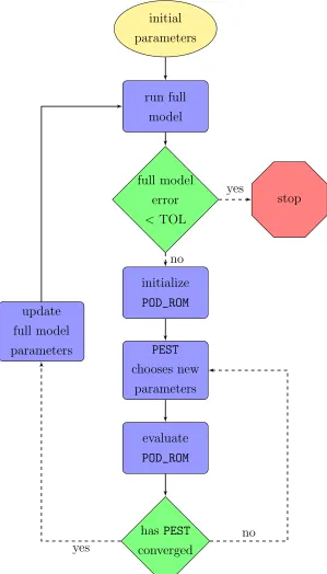
Algorithm
initial parameters
run full model
full model error
< TOL
stop
initialize POD_ROM
PEST
chooses new parameters
evaluate POD_ROM
has PEST converged update
full model parameters
yes
no
yes
no
1.
initial parameters
: The user must select the initial iterate. Our method has been shown to work even for very poor initial iterates. There is a danger of the Levenberg-Marquardt parameter estimation process finding a local minimum, but in our results that has not been the case.
2.
run full model
: We always run ADH or Mat_FEM first to generate the POD basis and gather the finite element matrix information. When the PEST optimization process has completed, we must rerun the full model to update the basis with the new information.
3.
full model error
<TOL
: We stop the parameter estimation process when the error between the full model and the given data (R from (6.2)) has converged or is less than some tolerance.
4.
initialize POD_ROM
: We only need to read in the information from the full model once for each PEST estimation loop. We use the same parallel partitioning in both ADH and POD_ROM. This allows each processor to read in information simultaneously, pseudo-parallelizing the I/O from the full model to the reduced model.
5.
PEST
chooses new parameters
6.
evaluate POD_ROM
: We emphasize that PEST uses only the output from POD_ROMto perform the optimization process. As such, a reduction in the POD_ROM residual does not necessarily translate to a reduction in the residual from the full model. In our results, the first solution from PEST often increases the residual from the full model. When this new information is included in the POD basis, however, PEST quickly converges to the correct solution.
7.
has PEST converged
: We discuss in Appendix D exactly what termination criteria we use inPEST. It is a mixture of iterations without sufficient improvement and absolute tolerance on the residual. If PESThas not yet found a solution, the parameters are updated and the reduced order model is again executed.
8.
update full model parameters
: Once the PESTalgorithm has found a set of parameters, the full model is run with the new conductivities. Only when the output from the full model is within an acceptable tolerance of the data do we terminate the process. Otherwise, the information from the full model is used to update the basis and we reenter the PEST optimization loop.
Chapter 7
Results
7.1
2-D Results
Description of Problem
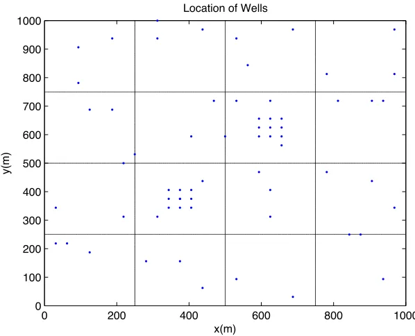
Our first implementation of POD on a groundwater system used a 2-D domain coded in Matlab. We use a 2-D finite element code distributed by Gockenbach [38]. The domain
is a square kilometer partitioned into sixteen equal sized material zones. We placed two pumping wells in the domain with a pumping rate set by the user. We implemented a hydraulic gradient along thex-axis using dirichlet boundary conditions at the x= 0 and
x= 1km boundaries and no flow conditions in they-direction at the y= 0 andy= 1km
0 200 400 600 800 1000 0
100 200 300 400 500 600 700 800 900 1000
Location of Wells
x(m)
y(m)
Figure 7.1: 2-D Domain with Sensors
0 200
400 600
800 1000
0 500
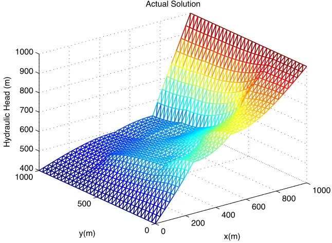
1000 400 500 600 700 800 900 1000
x(m) Actual Solution
y(m)
Hydraulic Head (m)
Figure 7.2: “Data” Solution with 4x4 Conductivity Grid
POD Solution
The purpose of the 2D investigation was as a “proof of concept” rather than a rigorous trial of POD performance. To that end, our results are limited in scope as they were only intended to demonstrate the potential of POD implementation on a saturated ground-water problem. There are no timings associated with this domain nor was it run on the HPC machines.
0 200
400 600
800 1000
0 500
1000400 500 600 700 800 900 1000
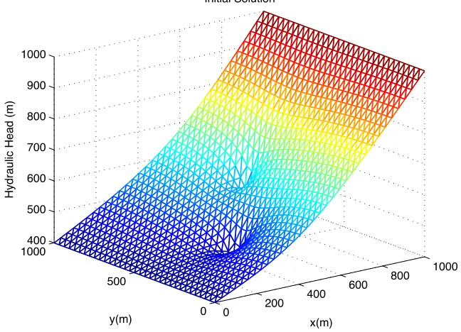
x(m) Initial Solution
y(m)
Hydraulic Head (m)
Figure 7.3: Initial Solution (Homogeneous Conductivity)
From this homogeneous solution, we extract the sensitivities ∂h
∂κi
as previously
dis-cussed and create the POD basisU =
h, ∂h ∂κi
0 2 4 6 8 10 12 14 16 18
10−25
10−20
10−15
10−10
10−5
100
Iterations
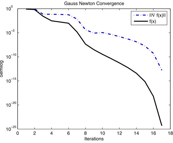
Semilog
Gauss Newton Convergence
||! f(x)||
f(x)
0 50 100 150 200 250 300 350
10−6
10−5
10−4
10−3
10−2
10−1
100
Iterations
Semilog
Levenberg−Marquardt Convergence
||! f(x)||
f(x)
0 200
400 600
800 1000
0 500
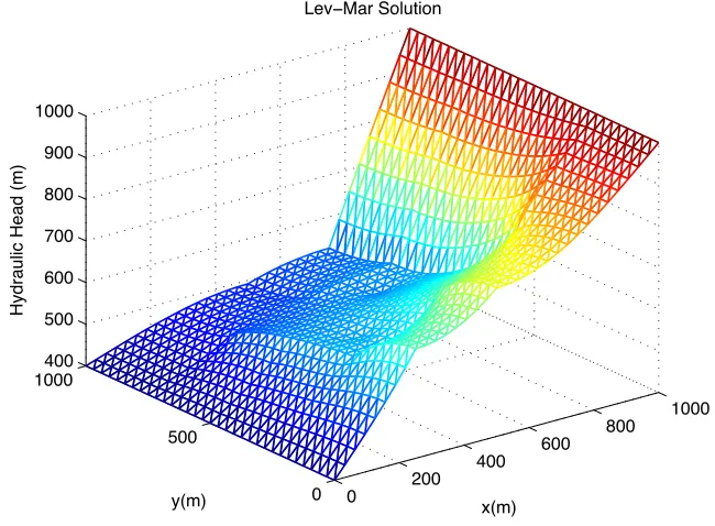
1000 400 500 600 700 800 900 1000
x(m) Lev−Mar Solution
y(m)
Hydraulic Head (m)
Figure 7.6: Levenberg-Marquardt Solution
Upon examining the iteration histories, we notice the LM code takes significantly more calls to the reduced function than GN. We are not concerned about this, however, as the reduced model function calls are so inexpensive it is a small computational investment to compute even several hundred iterations. What is significant is that both methods, GN and LM, were able to successfully reduce the error between the approximated model and the “data” solution to near zero.
From these results, we felt confident POD could be applied to more complex, 3-D domains. The following section demonstrates how POD has performed with such models.
7.2
3-D Results
7.2.1
Synthetic Column
location of the three materials in the column is shown in Figure 7.7. The column is discretized with a finite element mesh with 5,881 nodes and 30,720 tetrahedral elements. We create a hydraulic gradient with a Dirichlet condition at the bottom of the column and a flux at the top of the column. The vertical sides of the column have no-flow Neumann boundary conditions. These boundary conditions represent a thin column where hydraulic head is driven by gravity and an influx from the top. We are careful to ensure the flux through the boundary does not cause the column to become unsaturated.
Figure 7.7: Composition of Column
We synthesize the data by assigning conductivities and usingADHto create a solution. The data set is created with conductivities
~κ= [1.1808e−1,1.1808e−3,1.1808e−5](m/s).
the column as shown in Figure 7.9.
Figure 7.9: Location of Sensors
Our initial iterate is a homogeneous column, with ~κ = [1e−2,1e−2,1e−2]. Other initial guesses were chosen with no significant change in the behavior of the optimization process. The error between this iterate and the data is labelled as “Initial Residual” in Table 7.1. From this iterate, we generate the initial POD basis and start the Levenberg-Marquardt optimization process.
This increases the computational cost of POD as each full model access is expensive. Our goal is to recover the data solution using fewer full-model calls than would be required if the optimizer did not use the POD basis. When we display our results, we will show how many times the POD basis had to be reinitialized – the number of full-model calls – as well as how many times the optimizer used the reduced POD model. It should be noted that the POD model has a negligible contribution to computational effort in comparison to the cost of a full-model solve.
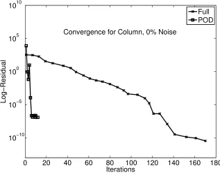
After we successfully recovered the solution for this synthetic column with zero-residual data, we increased the complexity of the problem by adding random “noise” to the data. We perturbed the data by a relative norm of 1%,5%, and 10%. As shown in Table 7.1, PEST reduced the objective function to a norm of similar magnitude when it queried only the POD model and when it used the full model. However, the optimization process with the POD model required significantly fewer full-model calls to obtain that solution. We see in Table 7.2 that the optimization process was able to recover the exact parameters when fed accurate data. With very noisy data, we see that PEST with both the reduced model and the full model was only able to recover two to three digits of the parameters. We also see in these results the clay “lens” (κ3) dominates the behavior of the column and is most accurately recovered with respect to the other parameters even with noisy data.
Table 7.1: Analysis for Column
Noise Model Full POD Initial Final Time Calls Calls Residual Residual (s)
0% POD 9 249 3.47E+02 6.00E-08 28
Full 170 - 4.37E-10 286
1% POD 7 268 3.49E+02 1.54E-02 31
Full 186 - 1.54E-02 352
5% POD 4 153 3.48E+02 4.24E-01 15
Full 152 - 4.22E-01 289
10% POD 6 187 3.61E+02 2.02 15
Table 7.2: Relative Log-Transformed Parameter Error for Column
Noise Model Relative Log-Parameter Error
|ln(κi)−ln(κest)|
|ln(κi)|
κ1 κ2 κ3
0% POD 2.37E-04 4.60E-07 2.93E-06
Full 2.46E-04 2.51E-07 3.73E-07
1% POD 1.00E+00 8.61E-03 6.40E-04
Full 1.00E+00 8.61E-03 6.41E-04
5% POD 1.00E+00 5.55E-02 1.62E-04
Full 9.78E-01 5.43E-02 7.80E-05
10% POD 2.40E-01 5.67E-02 5.93E-04
Full 1.08E+00 3.32E-02 1.08E-03 Actual ln(κi): -2.14E+00 -6.74E+00 -1.13E+01
0 20 40 60 80 100 120 140 160 180 10−10
10−5 100 105 1010
Iterations
Log−Residual
Convergence for Column, 0% Noise
Full POD
Figure 7.10: Convergence of Optimizer for 0% noise
The solutions from the POD approximation are visually indistinguishable from the generated data as shown in Figure 7.11.
(a) True Solution (b) Full Model Solution (c) POD Model Solution
The solution against noisy data shown in Figure 7.12 is very similar in behavior to the zero-residual case. We notice the scale of the solution has changed from the non-perturbed case.
(a) True Solution (b) Full Model, 10% Noise (c) POD Model, 10% Noise
7.2.2
Laboratory Scale Synthetic Aquifer
Our second application is a tank packed with five materials by Tissa H. Illangasekare and his team at the Colorado School of Mines (CSM) [81]. The container, pictured in Figure 7.13, is 208cm x 117cm x 57cm and divided into Cartesian blocks with 28,290 cells of material. To fill the tank, a mesh was placed at each level and each hole was filled with material. The mesh was then removed leaving a precisely packed domain. We can see the packing method in Figure 7.14 and the allocation of materials in Figure 7.15.
Figure 7.14: Packing Method
Flow through the domain was generated with Dirichlet boundaries on the two “short” sides of the tank. Figure 7.13 shows the gap on the near edge where the water height is maintained.
Figure 7.15: Allocation of Materials
Figure 7.16: Location of Sensors in Tank
sample points are shown in Figure 7.16. Our comparison against their measurements is labelled “Data” in Tables 7.3 - 7.4. We also synthesized data from the virtual represen-tation of the tank to generate a zero residual problem. That zero residual solution was perturbed by 1%, 5%, and 10% in order to test convergence with noisy data.
We see in Table 7.3 that PEST was able to recover a similar solution with both the reduced model and the full model. When it used the POD model, the number of full model calls was reduced by two orders of magnitude and the time to solution was reduced by an order of magnitude. As the noise was increased in the problem, the quality of fit deteriorated significantly. However, the reduced model provided a fit no worse in norm or parameter fit than the fit found with the full model. Table 7.4 shows the parameter fit was similar when the optimizer used either the reduced or full model for all noise levels. For this example, unlike the column, there is no single material that dominates the behavior of the domain. Figure 7.17 shows the optimizer behaves similarly for the tank as it did for the column.
Table 7.3: Results for CSM Tank with Direct Solver
Noise Model Full POD Initial Final Time Calls Calls Residual Residual (s)
0% POD 7 230 3.73E+03 1.34E-09 5.52E+03
Full 121 - 2.26E-05 7.92E+04
1% POD 3 80 3.74E+03 9.63 2.20E+03
Full 98 - 9.63 6.48E+04
5% POD 3 69 4.29E+03 2.55E+02 2.21E+03
Full 179 - 2.50E+02 1.18E+05
10% POD 3 49 4.62E+03 1.16E+03 1.42E+03
Full 103 - 1.14E+03 6.95E+04
Data POD 4 103 3.63E+03 2.67E-02 2.92E+03
0 20 40 60 80 100 120 10−10
10−5 100 105
Iterations
Log−Residual
Convergence for Tank, 0% Noise
Full POD
Table 7.4: Relative Log-Transformed Parameter Error for Tank
Noise Model Relative Log-Parameter Error
|ln(κi)−ln(κest)|
|ln(κi)|
κ1 κ2 κ3 κ4 κ5
0% POD 3.55E-06 7.47E-05 1.63E-06 6.27E-05 3.90E-04 Full 5.97E-04 6.27E-04 3.20E-03 1.67E-03 7.16E-03 1% POD 6.38E-02 4.64E-01 3.08E-01 2.23E-01 4.42E+00
Full 6.05E-02 4.37E-01 2.94E-01 1.80E-01 5.11E+00 5% POD 2.99E-01 6.72E-01 1.35E+00 7.97E-01 9.98E-01
Full 7.12E-01 2.38E+00 3.75E+00 8.54E-01 1.00E+00 10% POD 2.99E-01 2.36E-01 2.50E-01 6.76E-01 1.16E+01 Full 1.32E+00 4.97E-03 5.75E-01 3.51E+00 1.43E+01 Data POD 4.57E-01 5.06E-01 1.14E-01 8.50E-01 6.15E+00 Full 4.57E-01 5.06E-01 1.14E-01 8.50E-01 6.18E+00 Actual ln(κi): -5.01E+00 -3.89E+00 -2.76E+00 -1.64E+00 -5.16E-01
Figure 7.18: Exact Solution of Tank
(a) Full Model, 0% Noise (b) POD Model, 0% Noise
(a) Full Model, Measured Data (b) POD Model, Measured Data
7.2.3
SPE10
Our final example is from the Society of Petroleum Engineers Tenth Comparative Solution Project (SPE10) [19]. The model is specifically designed to test the limits of any methods attempting to use a fine grid implementaton due to its size and complexity. The domain is 1200×2200×170 feet and is split into 85 layers with five materials. Our mesh of the domain has 1.1 million nodes and 4.5 million elements. As shown in Table 8.1, it takes a desktop computer nearly 45 minutes for one full-model solve of SPE10. This in comparison to 40 seconds for the tank and just under two seconds for the column. The material allocation is shown in Figure 7.21.
Figure 7.21: Material Allocation for SPE10
The size of SPE10 forces us to use an iterative solver instead of a direct solver as we did with the previous examples. The effects of an iterative solver are explored in§8. We use a L2 norm tolerance of 1e−6 to achieve the following results.
Table 7.5: Relative Log-Transformed Parameter Error for SPE10
Solver Accuracy Model Relative Log-Parameter Error
|ln(κi)−ln(κest)|
|ln(κi)|
κ1 κ2 κ3 κ4 κ5
We see this table is consistent with the results of previous investigations; PEST with POD is able to achieve similar fits to parameters as PEST with the full ADH model. We see in Table 8.36 that the number of full model calls have been decreased by an order of magnitude and the time to solution has been cut in half ifPEST queries the POD model. However, the final residual and parameter error are similar.
Table 7.6: SPE10 Results for 1e−6 Solver Tolerance
POD Full
Time (s) 2.51e+04 5.26e+04 Final Residual 9.49e-04 9.31e-05 Parameter Error 2.10e-01 2.47e-01
ADH Calls 13 187
POD Calls 340
-As in previous results, the solutions from PEST with POD and PEST with ADH are nearly indistinguishable visually. Figure 7.22 displays the “true solution” of SPE10, generated with the correct conductivity values. Figure 7.23 shows the POD solution and the ADH solution. Due to the extreme size of SPE10, we used a different visualization software to display the results. The column and tank results are displayed with GMS[1] and SPE10 is visualized withParaView [44].
(a) SPE10 Solution withADH as Model (b) SPE10 Solution with POD as Model