DOI: 10.1534/genetics.108.091058
Mixed Effects Models for Quantitative Trait Loci Mapping With
Inbred Strains
Lara E. Bauman,*
,†,1Janet S. Sinsheimer,
†,‡,§Eric M. Sobel
§and Kenneth Lange
†,§,**
*Department of Genetics, Southwest Foundation for Biomedical Research, San Antonio, Texas 78245-0549,†Department of Biomathematics, University of California, Los Angeles, California 90095-1766,‡Department of Biostatistics, University of California, Los Angeles,
California 90095-1772,§Department of Human Genetics, University of California, Los Angeles, California 90095-7088 and**Department of Statistics, University of California, Los Angeles, California 90095-1554
Manuscript received May 14, 2008 Accepted for publication September 5, 2008
ABSTRACT
Fixed effects models have dominated the statistical analysis of genetic crosses between inbred strains. In spite of their popularity, the traditional models ignore polygenic background and must be tailored to each specific cross. We reexamine the role of random effect models in gene mapping with inbred strains. The biggest difficulty in implementing random effect models is the lack of a coherent way of calculating trait covariances between relatives. The standard model for outbred populations is based on premises of genetic equilibrium that simply do not apply to crosses between inbred strains since every animal in a strain is genetically identical and completely homozygous. We fill this theoretical gap by introducing novel com-binatorial entities called strain coefficients. With an appropriate theory, it is possible to reformulate QTL mapping and QTL association analysis as an application of mixed models involving both fixed and random effects. After developing this theory, our first example compares the mixed effects model to a standard fixed effects model using simulated advanced intercross line (AIL) data. Our second example deals with hormone data. Here multivariate traits and parameter identifiability questions arise. Our final example involves random mating among eight strains and vividly demonstrates the versatility of our models.
I
N analyzing gene mapping data from inbred strains, there is always the temptation to borrow models more pertinent to outbred populations. The vast major-ity of statisticians are wise enough to resist this temp-tation and turn to analysis methods tailored to specific breeding designs. Fortunately, the typical backcross or F2design has sufficient symmetry to permit analysis ofvariance by standard statistical packages. As mamma-lian geneticists explore more complicated designs in-volving multiple strains and multiple generations, this analysis paradigm has begun to fracture. It is therefore hardly surprising that the last decade and a half have seen a revival of interest in statistical models for gene mapping with inbred strains. Although we briefly re-view some of the important contributions to this lit-erature in the next section, it is fair to say that most modern models rely heavily on fixed effects. In contrast, the most successful models for mapping quantitative trait loci (QTL) in outbred populations invoke random effects (Hopper and Mathews1982; Goldgar1990; Schork
1993; Amos1994; Blangeroand Almasy1997).
The premise of this article is that, properly formu-lated, random effects models hold equal promise for more complicated inbred strain data. If a QTL is
seg-regating between two strains, backcross and F2designs
reliably detect it (Valdaret al.2006). Models based on
fixed allelic effects play a critical role in this process. Tra-ditional designs have two drawbacks. First, the scarcity of recombination events often gives long mapped intervals. Second, when two founder strains of related ancestry are chosen, there may be no segregating QTL. To increase the number of recombination events and the number of segregating QTL, geneticists are turning to more com-plex designs involving multiple strains. Although the rationale for more complex designs is compelling, they bring in their wake problems of overparameterization. Random effects models neatly circumvent some of the parameterization issues encountered with fixed effects models. Unfortunately, the standard outbred QTL model does not make sense for inbred strains. All individuals of a particular strain are genetically identical and completely homozygous. These cardinal character-istics have subtle consequences when we calculate trait covariances for the descendants of matings between different strains. A logically correct theory for specifying covariances between pairs of individuals is the key to making random effects models respectable for inbred strains.
In this article, we take two approaches to QTL mapping; both capture polygenic background as a source of random variation. The two approaches differ in how they handle variation caused by the QTL. In
1Corresponding author:Department of Genetics, Southwest Foundation for Biomedical Research, P.O. Box 760549, San Antonio, TX 78245-0549. E-mail: [email protected]
association mapping, markers are treated one by one as candidate genes, and observed genotypes or allele counts at a marker serve as fixed predictors of trait means. In linkage mapping, markers in the vicinity of the QTL provide prior information on gene sharing, and the QTL contribution is modeled as a random ef-fect. The greatest defect of our models is the blanket assumption of additivity. The greatest strength of our models is their generality in other regards. Thus, there is no limit to the number of founding strains, the depth and complexity of pedigrees, or the number of traits in a multivariate analysis.
To avoid breaking the flow of our discussion, much of the mathematical detail is relegated to theappendixes.
The following sections summarize previous contribu-tions, lay out the model with full attention to computa-tion of strain coefficients and relative covariances, resolve the thorny issue of identifiability, apply the mod-els to real and simulated data, and discuss the broader implications and limitations of the models.
METHODS
A brief survey of previous methods: Inbred
mam-malian strains have unique advantages in genetics. All members of a strain are genetically identical and com-pletely homozygous. Simple crosses between strains in-volve no phase ambiguities, and any genes mapped can be quickly located in humans and other species by synteny. With mice and other small mammals, breeding is reasonably straightforward, generation times are fairly short, and the environment can be exquisitely controlled. For decades, QTL mapping in inbred strains was considered an exercise in fixed effects modeling. Testing for association between marker genotypes and trait values is readily carried out using several available statistical packages. In the interval method introduced by Landerand Botstein(1989), the QTL is allowed to
take any position along a chromosome. This makes QTL genotypes unobservable and requires computation of posterior distributions given observed genotypes at the flanking markers. Although the EM algorithm is appli-cable in this context, it is often slow to converge, and the
regression method of Haley and Knott (1992)
pro-vides a quick approximation. The permutation test of Churchill and Doerge (1994) handles multiple
testing problems gracefully. The recent program R/qtl (Bromanet al. 2003), which capitalizes on the R
soft-ware environment, combines several of these methods with hidden Markov modeling of missing genotypes. Despite these admirable advances, interval mapping is still limited to simple crosses where polygenic back-ground is confounded with random environment. As the field embraces more complex crosses, geneticists no longer have the luxury of ignoring polygenic back-ground, and it seems self-evident that explicitly model-ing it will improve statistical inference.
The composite interval mapping method of Zeng
(1993, 1994) implemented in QTL Cartographer gen-eralizes interval mapping by including the direct effects of one or more markers unlinked to the QTL. Hence, composite interval mapping can be viewed as an attempt to incorporate polygenic background through fixed effects. If the number of typed markers is large, then it becomes hopeless to include all of them, and some automatic selection of background markers is desirable (Manlyand Olson1999).
Although Xieet al.(1989) take important first steps
toward including polygenic background as a random effect, they do not derive general covariance expres-sions. This failure makes it difficult to deal with non-standard crosses and awkward to combine data from different crosses. In the meantime, the pressure to in-crease the number of strains per cross has been growing (Rebaiand Goffinet1993). Of 21 cloned mouse genes
listed in Tables 1 and 2 of the review by Flint et al.
(2005), 7 rely on cloning strategies involving multiple strains or outbred mice. These practical concerns are stimulating intense efforts to revamp experimental design and statistical analysis of inbred cross data (Liu
and Zeng2000; Hitzemannet al.2002; Pletcheret al.
2004; Liet al.2005; Cervinoet al.2007). Other recent
models that delve into multiple QTL models and epis-tasis are both frequentist (Kaoet al.1999; Janninkaand
Jansena2001; Seatonet al.2002; Bromanet al.2003)
and Bayesian oriented (Sillanpa¨ a¨and Arjas1998; Sen
and Churchill2001; Bromanet al.2003).
Trait means, variances, and covariances: We begin our theory development with a basic model applicable to any inbred strain design, including F2, advanced
intercross lines, and random mating. Suppose thatiand
jare two animals generated by a complex cross involving
s inbred strains. At t traits of interest, i and j exhibit random vectors Xi and Xj of trait values. For the sake of simplicity, assume further thatXiandXjreflect the contributions of a single gene whose alleles have ad-ditive effects. Our immediate goal is to calculate the expected vectors E(Xi) and E(Xj) and the covariance matrix Cov(Xi,Xj). Wheni¼j, we recover variances as well as covariances. Because of our assumption of ad-ditivity,Xidecomposes as the sumYi1Ziof a maternal contribution Yi plus a paternal contribution Zi. To calculateE(Yi), let Midenote the originating strain of the maternal gene ofi. AlthoughMiis unobserved, we can calculate the probability Pr(Mi¼a) for any given straina. In terms of these probabilities and thet 3 1 mean vectorm(a) of allelic effects on each trait for strain
a, we have
EðYiÞ ¼
Xs
a¼1
PrðMi ¼aÞmðaÞ:
EðXiÞ ¼2
Xs
a¼1
giðaÞmðaÞ; ð1Þ
wheregi(a) is the probability that a randomly sampled
gene fromioriginates from straina. We refer togias the
strain fraction vector for animali;gihas dimensions31.
Covariances are derived by the same kind of reason-ing. DecomposeXjinto the sumVj1Wjof a maternal contributionVjplus a paternal contributionWj. In view of the bilinearity of the covariance operator and the symmetry of maternal and paternal alleles, it suffices to find the covariance Cov(Yi, Vj). Let Nj denote the originating strain of the maternal gene ofj. Condition-ing on the joint value ofMiandNjthen yields
CovðYi;VjÞ ¼EðYiV*jÞ EðYiÞEðVjÞ*
¼X
a
X
b
PrðMi ¼a;Nj ¼bÞmðaÞmðbÞ*
X
a
PrðMi ¼aÞmðaÞ
" #
3 X
b
PrðNj¼bÞmðbÞ
" #*
;
where the superscript * indicates a vector or matrix transpose. By analogy with kinship coefficients, we define the strain coefficient cij(a, b) to be the joint
probability that a randomly drawn gene from animali
originates from strain a and a randomly drawn gene
from the same locus of animaljoriginates from strainb. If i and j coincide, then sampling is done with re-placement. Thet3tcovariance matrix between the trait values ofiandjbecomes
CovðXi; XjÞ ¼CovðYi;VjÞ1CovðYi;WjÞ1CovðZi;VjÞ
1CovðZi;WjÞ
¼4X
a
X
b
cijða;bÞmðaÞmðbÞ*
4X
a
giðaÞmðaÞX
b
gjðbÞmðbÞ*
¼4X
a
X
b
Cijða;bÞmðaÞmðbÞ*; ð2Þ
whereCij(a,b)¼cij(a,b)gi(a)gj(b), which we collect
into ans3smatrix, denotedCij.
Forsstrains andttraits, it is convenient to stack the allelic effects into a column vectormof lengthst with transpose
m*¼ ½m1ð1Þ;. . .;m1ðsÞ;. . .;mtð1Þ;. . .;mtðsÞ: The positive semidefinite matrixV¼mm* can then be split intot2blocksV
kleach of sizes3s. Restricting our
attention to the block corresponding to traitskandl, the covariance matrix (2) has entries given by the trace formula
CovðXik;XjlÞ ¼4 trðCijVklÞ: ð3Þ
In polygenic inheritance, many independent loci contribute in an additive manner to the traits under consideration. Since trait means and covariances add in this setting, the mean expression (1) and the covariance expressions (2) and (3) remain valid provided we replacembyPlmlandVbyP
lmlðmlÞ*. Herem
ldenotes
the vector contribution corresponding to locuslrather than the lth component of m. appendix a shows that
every pair (m,V) consisting of a vectormand a positive semidefinite matrixVcan be represented as two such coordinated linear combinations. Hence, to capture polygenic background, it suffices to estimate arbitrarym
andV. We see later that there is an identifiability issue that must be surmounted in estimatingV.
Computation of strain coefficients: Because the
combinatorial coefficientsgi(a) andcij(a,b) are essen-tial in calculating trait means and variances, we need good algorithms to compute these coefficients. Fortu-nately, we can mimic the logic used in calculating kinship coefficients for outbred populations. Since a pedigree founder i is assumed to be strain pure, one entry of the vectorgi¼1, and the remaining entries¼0.
Likewise for two foundersiandj, one entry of the matrix
cij¼1, and the remaining entries¼0. All other strain
fraction vectorsgiand strain coefficient matricescijare
defined recursively starting with the founders.
To avoid circular reasoning, pedigree members are numbered so that parents always precede their children. If animaliis not a founder, then it has parentskandl. Assuming thatkandlhave already been visited in filling in the strain fractions, we set
gi¼1
2ðgk1glÞ: ð4Þ
Ifj6¼i, then without loss of generality we can assumej
has been visited already, and we can set
cij¼1
2ðckj1cljÞ ð5Þ
cji¼1
2ðcjk1cjlÞ: ð6Þ
This leaves only the casej ¼i. There are four equally likely possibilities when we sample two genes of i: (a) both genes coincide with the gene passed byk, (b) both genes coincide with the gene passed by l, (c) the first gene comes fromkand the second froml, and (d) the first gene comes from land the second fromk. These considerations produce the matrix recurrence
cii¼1
4½diagðgkÞ1diagðglÞ1gkgl*1glgk*; ð7Þ
The initial conditions on founders and the recurren-ces (4)–(7) completely determinegi andcij. These in
turn determine the Cij matrices, which have a richer mathematical structure than the strain coefficient ma-trices cij. appendix b describes several fascinating
properties of the Cij matrices. One such property is
Cij ¼0 between most members of simple crosses, for example, for all F2animals wheni6¼jor wheneveriis a
founder or F1.
Variance component models for QTL mapping with outbred populations require conditional kinship coef-ficients in addition to theoretical kinship coefcoef-ficients. For exactly the same reasons, we also need conditional strain fractions and coefficient matrices. These depend on observed marker genotypes in the vicinity of a putative QTL. On small pedigrees, it is possible to compute conditional strain coefficient matrices exactly by considering all descent graphs (gene flow patterns) at the QTL and neighboring markers (Kruglyaket al.
1996). In practice, inbred strain pedigrees are so large that the number of possible descent graphs is astro-nomical. Stochastic sampling provides a workable sub-stitute for exhaustive enumeration of descent graphs
(Sobel and Lange 1996). The Markov chain Monte
Carlo (MCMC) method incorporated in the computer program SimWalk samples relevant descent graphs with the appropriate conditional probabilities. Given a de-scent graph at the QTL, it is trivial to compute strain fractions for all animals and strain coefficient matrices for all pairs of animals in a pedigree. The averages of these quantities over all sampled descent graphs serve as approximations to the conditional strain fractions and strain coefficient matrices.
Strain coefficients convey more information than strain fractions. For instance, it is obvious that
giðaÞ ¼X
b
ciiða;bÞ:
We can put this extra information to good use in predicting QTL genotypes. At a given genomic location, imagine a marker with a different allele for each strain. Let ˆbiða=bÞbe the conditional probability that animali
has unordered genotypea/bat the hypothetical marker given the observed data at the ordinary markers. The relations
ˆ
ciiða;aÞ ¼1 2gˆiðaÞ1
1
2bˆiða=aÞ; ˆ
ciiða;bÞ ¼1
4bˆiða=bÞ;b 6¼a
connect the conditional genotype probabilities to the conditional strain fractions and coefficients. These relations in turn imply that
ˆ
biða=aÞ ¼2 ˆciiða;aÞ gˆiðaÞ; ˆ
biða=bÞ ¼4 ˆciiða;bÞ;b6¼a: ð8Þ
Thus, we can impute strain genotypes as well as strain fractions.
Variance component models: Variance component
models revolve around the multivariate normal distri-bution or related distridistri-butions such as the multivariatet. Every multivariate normal distribution is uniquely de-termined by its mean vectornand variance matrixS. If we decompose trait values into independent, additive contributions, thennandScan be expressed as sums over the various contributions. As long as we are willing to take the leap of faith that all random contributions are Gaussian, then trait vectors will be Gaussian as well. For each random contribution, variance matrices are constructed from a constant part and a parametric part. The genetic covariance formula (3) is typical in this regard. The constant partsCijare forced on us by the
nature of the pedigree. The parametric part V with
blocksVklrequires estimation.
The environmental contribution to the mean is
usually modeled as the sum of a grand mean h plus
covariate effects such as age or sex. Random environ-ment and cage effects can be modeled by Kronecker products of variance matrices, provided we order trait values so that all values corresponding to a given trait are contained in a single block, and animals are consistently enumerated across blocks. Given these conventions, the variance matrix under random environment reduces to the Kronecker productY5Iof the trait variance matrix
Y and the identity matrix I. Obviously, Yis the para-metric part; it describes the environmental covariation of the traits in a single animal. The matrix I reflects the independence of the random environments for the various animals. For a random cage effect, we replace the identity matrix by a cage matrixH¼(hij), wherehij¼
1 if animals i and j belong to the same cage and 0
otherwise. The matrix replacingY describes the envi-ronmental covariation of the traits for animals in a single cage (Lange 2002). As an example, heritability
analyses generally specify two random effects, additive polygenes and random error/environment,
EðXikÞ ¼2
Xs
a¼1
giðaÞmkðaÞ1 X
C
c¼l
aicbkc1h ð9Þ
CovðXik;XjlÞ ¼4 trðCijVklÞ1Ykl; ð10Þ
whereaicis thecth ofCcovariates measured on animali
andbkcis the corresponding regression coefficient for traitk.
Once we specify the mean and variance components, the loglikelihood of a pedigree can be written as
L ¼ 1
2ln detS
1
2ðxnÞ*S
1ð xnÞ;
independently, their loglikelihoods add. Given the over-all loglikelihood, parameters can be estimated by max-imum likelihood, and statistical inference conducted by standard likelihood ratio tests comparing alternative hypotheses to null hypotheses. Lange(2002) develops
this frequentist approach to estimation and inference in detail. Our computer program Mendel relies on a quasi-Newton algorithm for maximum likelihood estimation. Bauman et al.(2005) discusses an alternative EM
algo-rithm as well as factor-analytic parameterizations of variance matrices. Given the presence of covariates and heterogenous pedigree structures, permutation testing is rarely possible. To aid the user in judging significance and model fitting, Mendel reports standard errors of parameters, pedigree deviances, outlier individuals, and various goodness-of-fit statistics.
Two QTL mapping strategies:There are two specific strategies, association and linkage, for QTL mapping. Variance component models are pertinent to both. Although the two strategies differ in how they portray QTL effects, each captures polygenic background as a random effect. In addition to the strain effects appear-ing in Equation 1, most models include a grand meanh
and fixed effects tied to plausible predictors. If we specify h, then we must impose the vector constraint P
amðaÞ ¼0on the polygenic mean vectorm. Here the
indexaranges over all strains. Random effects include the polygenic effect summarized by Equation 3, random environment plus measurement error, and possibly correlated environment such as cage effects. As de-scribed in the next section, the polygenic variance
matrix V is not identifiable, and complicated
con-straints must be imposed on it to compensate for this fact. Regardless of the nature of these constraints, we must compute theoretical strain fractions and strain
coefficients to estimate m and V under the null
hypothesis of no QTL effect.
In linkage mapping, markers serve to tag chromo-some segments and keep track of recombination events. The genotypes of the causative QTL are unobserved, and the QTL is allowed to assume any position along the genome. Under the alternative hypothesis in linkage mapping, we model the QTL as a random effect in the same way that we modeled the contribution of a single gene with additive effects. The only difference is that we use strain fractions and coefficients calculated condi-tional on the observed marker data. From here on, we refer to these as conditional strain fractions and coefficients; those calculated unconditionally we call theoretical strain fractions and coefficients. Motivated by Equations 1 and 3, we lete(a) denote the additive effect of the QTL in straina. Then our earlier reasoning shows that the QTL contribution has mean
2X
a
ˆ
giðaÞeðaÞ
for animaliand covariance
4X
a
X
b
c
Cijða;bÞeðaÞeðbÞ*
for animals i and j. Here the circumflexes indicate conditional versions of the strain fractions and coef-ficients estimated from the marker data. Under the alternative hypothesis, we estimate the entries ofe.
Our basic linkage model therefore specifies the trait means and covariances
EðXikÞ ¼2X
s
a¼1
giðaÞmkðaÞ12X
s
a¼1
ˆ
giðaÞekðaÞ1 X
c
aicbkc1h
ð11Þ
CovðXik;XjlÞ ¼4 trðCijVklÞ1trðCiˆjekel*Þ11fi¼jgYkl
ð12Þ
for two animalsiandj. Herekandlindex two traits,aic
is covariatec of animali, andbkcis the corresponding
regression coefficient for traitk. If we letedenote the averageð1=sÞPaeðaÞ, then all QTL models that include a grand mean require the constraint e¼0. In the presence of this constraint, the likelihood ratio test of linkage follows asymptotically ax2distribution withstt
degrees of freedom.
In association mapping, QTL fixed effects are tied to the current marker. The marker is viewed as a candidate gene whose genotypes or alleles directly influence trait
means (Lange et al. 2005); random QTL effects are
omitted. Hence, in Equation 12 we drop the random effect trðCijcekel*Þ, and in Equation 11 we amend the
fixed effect 2Psa¼1gˆiðaÞekðaÞ to represent regression
on observed allele counts at the current marker. If the additive model for allelic effects is viewed as too restrictive, then we can regress on observed genotypes. Association testing is again conducted by likelihood ratio statistics.
In the presence of missing genotypes in association testing, we fall back on imputed allele counts or im-puted genotype counts. Because genotypes at markers are usually directly observed, little is lost in imputation by ignoring genotypes at flanking markers. In this simpler setting, a fast deterministic algorithm is avail-able for imputation (Langeet al.2005). Flanking
mark-er genotypes occasionally resolve phase ambiguities caused by combining closely spaced single nucleotide polymorphisms (SNPs) into supermarkers. Accordingly, the current version of Mendel also accepts MCMC estimates of conditional strain fractions from SimWalk. When each strain carries a different allele at the marker, the allele counts delivered by SimWalk are computed by doubling the conditional strain fractions at the marker. When two strains share a common allele at the marker, the corresponding strain fractions are added before doubling.
traitlof animaljinvolves thes3strait blockVklof an st3stvariance matrixV. Unfortunately, estimation of
Vcollides with an identifiability issue. The crux of the problem is the existence of nontrivial matricesLwith
tr½CijðVkl1LklÞ ¼trðCijVklÞ
for every legitimate choice ofCijand every trait pair (k,
l). Proposition 2 ofappendix b explains this
phenom-enon by representingCijas a convex combination of the matrix 0 and ðs
2Þ matrices Emn indexed by unordered
strain pairs {m,n}. Here all entries ofEmnare 0 except for the diagonal entriesemm¼enn¼1 and the off-diagonal entriesemn¼enm¼ 1. It follows that
trðCijLklÞ ¼
X
fm;ng
aij;mntrðEmnLklÞ ¼0
provided
trðEmnLklÞ ¼lkl;mm1lkl;nnlkl;mnlkl;nm ¼0 ð13Þ
for every strain pair {m,n} and everys3strait blockLkl¼ (lkl,mn) ofL.
We can solve the identifiability problem by subtract-ing the nonidentifiable part ofVfromV. To achieve this end, we view the positive semidefinite matrixVas a vec-tor in the Euclidean spaceRst3st. In this setting the trace
function ,A;B. ¼ tr(AB*) and Frobenius norm
kAkF¼tr(AA*)1/2reduce to the standard inner product
and Euclidean norm. To find the nonidentifiable part of V, one projects V onto the vector subspace S of symmetric matrices satisfying Equation 13 for every strain pair {m, n} and every trait block Vkl. Formally,
the projectionP(V) is defined to be the matrixXgiving the minimum ofkVXk2FforX 2 S.
Fortunately, minimization ofkVXk2Fseparates into
subproblems corresponding to different trait blocks. First, consider a diagonal block Vkk of V. To simplify
notation, denote its entries by ymn ¼ Vkk,mn and the
entries of the corresponding block of the projection by
xmn ¼P(V)kk,mn. To findP(V)kkwe must minimize the
sum of squares
1 2
X
m
X
n
ðymnxmnÞ2
subject to the constraintsxmm1xnn¼xmn1xnmfor every pair {m,n}. Now consider off-diagonal blocksVkl¼Vlk*.
These come in pairs that must be handled together, so we let
ymn ¼Vkl;mn¼Vlk;nm
and
xmn ¼PðVÞkl;mn ¼PðVÞlk;nm
and minimize the sum of squares
1 2
X
m
X
n
ðymnxmnÞ21
1 2
X
m
X
n
ðynmxnmÞ2
¼X
m
X
n
ðymnxmnÞ2
subject to the constraintsxmm1xnn¼xmn1xnmfor every pair {m, n}. It follows that diagonal blocks and off-diagonal blocks lead to the same constrained minimi-zation problem.
appendix c shows that each of these least-squares
problems has solutionX¼(xmn) with residual
YX ¼1
2ðU1U*Þ;
whereY¼(ymn),U¼QYQ, andQis thes3sprojection matrixI ð1=sÞ11*. In calculating a covariance, we can ignore symmetrization and replace the matrix12ðU1U*Þ byU. Indeed, the symmetry ofCijimplies that
1
2tr½CijðU 1U*Þ ¼ 1
2trðCijUÞ1 1
2trðCijU*Þ ¼trðCijUÞ:
Thus, tr(CijQVklQ) faithfully represents the covariance between traitkof animaliand traitlof animalj. By the same reasoning, we can replace the entire residual ma-trixVP(V) by the matrix
R ¼diagðQÞVdiagðQÞ: ð14Þ
Here diag(Q) is a diagonal block matrix with all t
diagonal blocks equal toQ. One can easily check that diag(Q) is a projection matrix and thatR inherits the properties of symmetry and positive semidefiniteness fromV.
In reparameterizingV, it is convenient to define an orthogonal matrixOmapping the vectorð1=pffiffisÞ1to the standard basis vectore1. (Seeappendix dfor one version
ofO.) It follows that
OQO*¼OðI 1
s11*ÞO*¼I e1e1*:
Observe that pre- and postmultiplying any square matrix by I e1e1* zeros out the first row and first
column of the matrix. To take advantage of this fact, we express the residual matrix (14) as
R¼diagðO*ÞdiagðOQO*ÞdiagðOÞVdiagðO*ÞdiagðOQO*ÞdiagðOÞ ¼diagðO*ÞYdiagðOÞ: ð15Þ
The matrix
Y¼diagðOQO*ÞdiagðOÞVdiagðO*ÞdiagðOQO*Þ
is a positive semidefinite replacement for diag(O)V
diag(O*). By our earlier remark, a blockYklofYequals
the corresponding block of diag(O)Vdiag(O*) with its first row and column zeroed out.
columns consisting of zeros. Permuting its rows and columns appropriately will move its nontrivial part to an upper-left block, which will be positive definite when-everVis positive definite. The Cholesky decomposition of this upper-left block then serves as a good parame-terization ofR. To compute the number of parameters forsstrains andttraits, observe that the matrixYisst3 st. A total oftrows and columns are lost in the zeroing-out process. This leaves an (stt)3(stt) upper-left block with (stt)(stt11)/2 diagonal or subdiagonal entries. For example, with three strains and two traits, there are 10 parameters.
For the sake of clarity, let us summarize how our proposed parameterization leads to trait covariances. It begins with a Cholesky decompositionDof an (stt)3
(stt) positive definite matrix. The matrixDD* is then subdivided into (s1)3(s1) trait blocks (DD*)kl,
and each block is promoted to ans3strait blockYkl
by adding a top row and left column of zeros. In matrix notation,Ykl¼Z(DD*)klZ* withZthes3(s1) matrix
Z ¼ 0*
I
:
Finally, we construct the residual matrixRvia Equation 15, using the orthogonal matrixO.
With these conventions, the covariance between trait
kof animaliand traitlof animaljamounts to
CovðXik;XjlÞ ¼4 trðCijRklÞ
¼4 trðCijO*YklOÞ
¼4 tr½CijO*ZðDD*ÞklZ*O
¼4 tr½Z*OCijO*ZðDD*Þkl: ð16Þ
In computing covariances over large pedigrees, it saves time and storage to precompute and store the (s1)3
(s 1) matrices 4Z*OCijO*Z and discard the s 3 s
matricesCij. Note that the actionA1Z*AZon ans3s
matrixAdeletes the first row and first column ofA. This ends our theoretical overview of the model.
appendix eshows how to differentiate covariances with
respect to parameters, and appendix f supplies a
counterexample connecting identifiability and symme-try. We now move on to data analysis.
APPLICATIONS
A simulated advanced intercross line:An AIL starts with F1 offspring from an intercross of two inbred
strains. The F1animals are randomly bred to produce
the F2 animals, the F2 animals are randomly bred to
produce the F3 animals, and so on for a total of n
generations. An AIL differs from repeated brother– sister mating, because it involves enough animals to preserve genetic diversity. It draws its strength from the steady accumulation of recombination events over many generations (Darvasiand Soller1995).
Simu-lating data according to an AIL design permits us to compare our mixed effects results with the fixed effects results of the benchmark program QTL Cartographer. This exercise is not meant to be a substitute for an exhaustive study of power and experimental design. Also, the comparison is not entirely fair because QTL Cartographer analyzes the Fndata at the last generation
ignoring the previous generations. To reconstruct miss-ing marker information, QTL Cartographer applies an inflated recombination fraction scaled to reflectn.
To create our simulated AIL data, we mated two inbred founder animals and subjected their descend-ants in each generation to virtual random mating. Generation 10 contained 175 animals in 140 sibships with 492 animals overall. Placing the QTL locus at the midpoint of markers 5 and 6 of 11 equally spaced marker loci, we simulated genotypes by gene dropping and assigned QTL effects on the basis of the genotypes at the QTL. QTL genotypes were then discarded from further analysis. We modeled a univariate trait with a grand meanh¼4, an environmental variances2
env¼1,
and a 232 polygenic variance matrix
V¼ 1:0 0:20 0:20 0:29
:
For this simulated trait, strain one has a genetic variance comparable to the environmental variance and larger than the genetic variance of strain two. The two strains share a modest genetic correlation. For reasons ex-plained in the next section, a single generation of data in a symmetric cross of this sort does not sustain estimation of strain-specific polygenic means. To cir-cumvent this problem in our comparisons, we set the strain-specific polygenic means equal to 0. We chose small strain-specific QTL effectse1¼0.2 ande2¼ 0.2
centered around 0. In view of our discussion of identifi-ability, we can estimate only a single parameter p1
characterizing V. The projection technique discussed yields the value p1 ¼ 0.667. The discussion of the Cij
matrices inappendix bexplains why genotype data on a
single generation also prevent estimation ofp1.
To provide the most informative comparisons, we ran three analyses: (1) Mendel on the full pedigree with complete genotype and phenotype data (Mendel Full), (2) Mendel on the full pedigree but with phenotype data on only the final F10generation (Mendel F10), and
(3) QTL Cartographer on the final F10generation with
complete genotype and phenotype data (Cartogra-pher). Simply comparing cases Mendel Full and Car-tographer is hardly fair; the full pedigree contains more than twice the number of animals in the final genera-tion. Mendel F10takes advantage of the full genealogy
Before turning to QTL mapping in the Mendel analyses, we fit a baseline model including the grand mean, the polygenic variance, and the environmental variance. We then estimated conditional strain coeffi-cients at each of the 11 marker loci. This put us in a position to estimate the global parameters and the QTL-specific parameters simultaneously at each locus. The evidence in favor of the QTL is summarized by a likelihood ratio test (LRT) statistic following a x2 1
distribution; a nonlinear false discovery rate (FDR) correction (Benjaminiet al.2001) corrects for multiple
testing for all three analyses. Table 1 summarizes the type I error rate, power, and coverage as well as the generating parameters, their estimates, and the stan-dard errors of the estimates at the loci adjacent to the QTL. Successful coverage occurs when the equivalent one-LOD drop interval (4.6 LRT units) includes the QTL. We reject the null hypothesis of no QTL effect when the LRT is significant at the 0.05 level.
The results in Table 1 reflect 100 simulations for a QTL-effect size that yields power.90% for Mendel Full; type I error rates are given as confidence intervals based on 500 simulations under the null hypothesis of no QTL effect. Clearly, the power to detect linkage is drastically reduced when only the F10generation is available for
analysis. This absence of data also makes it difficult for
Mendel F10 to estimate the polygenic parameter p1
accurately. For Mendel Full all estimates are within one standard error of their true values, and standard errors are small. QTL Cartographer exhibits slightly better power and coverage than Mendel F10, but with a largely
inflated type I error rate. Both methods are easily bested by Mendel Full. These trends continue over a range of smaller QTL effects (data not shown). We are pleased with these results. In our view they demonstrate that applica-tion of the mixed effects model sacrifices little in simple settings while generalizing readily to complex pedigrees.
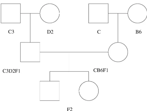
A multivariate four-way cross: To illustrate the anal-ysis of multivariate traits, we next consider the hormone data of Burke and colleagues (Harperet al.2003) on
aging HET3 mice. Figure 1 shows how the UM-HET3 mice were created from four founder strains: BALB/cJ (C), C57BL/6J (B6), C3H/HeJ (C3), and
DBA/2J (D2). CB6F1 females crossed with C3D2F1
males provided 967 F2 full siblings. At markers with
four different alleles, all F2 mice were heterozygous.
Thus compared to a two-way cross, the four-way cross doubles the number of founder strains without sacrific-ing phase certainty. Hormone levels of insulin-like growth factor I (IGF), leptin (Lep), and thyroxine (T4) were measured at 4 and 15 months on each of the F2 mice. Testing maternal and paternal effects
separately, Harperet al. found several linked markers in these data via ANOVA, including a maternal allele at D3Mit25 linked to IGF at 15 months, a paternal allele at D3Mit127 linked to Lep at 4 months, and both maternal and paternal alleles linked to Lep at 15 months. It is
worth pointing out that ANOVA or MANOVA must be carried out at marker loci. Only here do marker geno-types or allele counts unambiguously define factor levels. With complete genotyping, our model collapses in this setting to the classical models.
This multistrain cross highlights identifiability pitfalls inherent in the structure of some crosses and the data collected on them. For example, all F2mice share the
strain fraction vector141. Hence, the polygenic mean is confounded with the grand mean. Using strain trait averages or phenotyping members of the original strains would allow us to estimate the polygenic means, but this is not an option for the current data.
Although the rigid structure of the four-way cross preserves phase certainty, it reduces uncertainty to the point where the polygenic covariance matrix cannot be estimated. Polygenic covariances depend on the com-binatorial matricesCij. We have already noted thatCij¼
0 whenever i is a founder or i and j are F1 mice.
Straightforward calculations for F2miceiandjwithi6¼ jyield
Cij¼0; Cii¼
1 16
1 1 0 0
1 1 0 0
0 0 1 1
0 0 1 1
0 B B @ 1 C C A:
Inspection of Equation 3 therefore shows that the polygenic covariance matrixVis confounded with the matrix describing the environmental covariances.
Finally, there are identifiability problems with the QTL allelic effects. At the covariance level, the condi-tional coefficient matrixCijcis identically 0 when typing is full and different alleles are present in each strain. At the mean level, imposition of the constrainte4¼ e1
e2 e3 shows that the genotype-specific means in a
purely allelic model can be expressed as the vector
e11e31h
e11e41h
e21e31h
e21e41h
0 B B @ 1 C C A¼
1 0 1 1
0 1 1 1
0 1 1 1
1 0 1 1
0 B B @ 1 C C A e1 e2 e3 h 0 B B @ 1 C C A:
Because the matrix on the right of this equation has less than full rank, some mean vectors are not representable. As a substitute for the additive QTL contributions, we assign a different mean effect to each of the four F2genotypes.
We analyze these data in the same manner as the simulated AIL except for graphing thelog10(P-value)
instead of LRTs and analyzing multiple map points in the intervals between marker loci. We enjoy two advan-tages over ANOVA or MANOVA; namely, we can use phenotyped individuals with wholly or partially missing genotypes, and we can estimate both QTL location and effect size.
multiple testing problem and may add noise and degrade power (Amoset al.2001; Baumanet al.2005).
With outbred populations it is intertwined with the issue of ascertainment (Dawson and Elston 1984); it may
also be a problem with inbred populations since strains are often chosen for a particular experiment on the basis of their average phenotype. We present here the results of two multivariate analyses making these points. The most interesting results from this example data set
are on chromosome 3, and we focus on three traits, leptin measurements at both 4 and 15 months and insulin-like growth factor I at 15 months in this region. In univariate analysis, both IGF-15 and Lep-4 show significant linkage to markers on chromosome 3, while Lep-15 shows suggestive linkage. Multivariate analyses are indicated biologically, spatially, and temporally.
We carried out a number of multivariate analyses; some of the results are summarized in Figures 2 and 3 and Table 2. The graphs oflog10(P-value) along
chro-mosome 3 in Figure 2 correspond to the univariate an-alyses of IGF-15, Lep-4, and Lep-15 and the bivariate analysis of Lep-4 and Lep-15. The univariate graph of IGF-15 peaks over marker D3Mit5. Subjecting the
P-values for IGF-15 to the nonlinear FDR correction (Benjaminiet al. 2001) suggests a single location for
IGF-15. Both of the univariate leptin graphs as well as the bivariate graph peak over D3Mit127. After FDR correction, at least two significant map points are suggested over D3Mit127 for the bivariate leptin anal-ysis. Table 2 reports estimates and standard errors for the bivariate leptin mean parameters at marker D3Mit127. These estimates are very similar at the two time points. Although likelihood ratios improve over univariate analysis,P-values do not because the degrees
of freedom of the x2 test double. The estimated
environmental covariance matrix
ˆ
Se ¼ 0:96ð0:05Þ 0:50ð0:04Þ 0:50ð0:04Þ 0:97ð0:05Þ
ð17Þ TABLE 1
AIL: type I error, power, coverage, and average estimates
Mendel Full Mendel F10 Cartographer True value
Type I error 0.83–3.39 4.92–9.60 25.6–33.8 NA
Power 96 46 51 NA
Coverage 92 39 48 NA
Point 5
h 3.9913 (0.2058) 3.9661 (0.2355) NA 4.000
p1 0.6486 (0.1183) 0.3259 (0.0878) NA 0.667
e1 0.1910 (0.0487) 0.1759 (0.0764) 0.1869 0.200
e2 0.1910 (0.0487) 0.1759 (0.0764) 0.1869 0.200 s2
env 1.0112 (0.1002) 1.1494 (0.1721) 0.9581 1.000
Point 6
h 3.9998 (0.2059) 3.9465 (0.2344) NA 4.000
p1 0.6492 (0.1176) 0.3370 (0.0967) NA 0.667
e1 0.1932 (0.0477) 0.1764 (0.0758) 0.1781 0.200
e2 0.1932 (0.0477) 0.1764 (0.0758) 0.1781 0.200 s2
env 1.0092 (0.0998) 1.1458 (0.1746) 0.9606 1.000
Type I error rates, power, and coverage are percentages; estimates and standard errors are averages. Type I error rates are con-fidence intervals based on 500 simulations under the null hypothesis; other table entries are based on 100 simulations under the alternative hypothesis. We count successful coverage when the equivalent one-LOD drop (4.6 LRT units) interval around a sig-nificant map point includes the QTL. The QTL is located at the midpoint of points 5 and 6. Parameterp1is the reduced-dimension polygenic background parameter;h, the grand mean;ei, the QTL effect on straini; ands2env, the residual covariance. The Mendel estimates have average standard errors in parentheses. NA, not applicable.
is consistent with the raw correlation of the two traits. In the matrix (17), the standard error of each estimate appears in parentheses.
A trivariate analysis of IGF-15, Lep-4, and Lep-15 clearly illustrates that in the case of multivariate traits, more is not always better. Comparing Figure 2 to Figure 3 shows two large peaks: one at marker D3Mit25 and one over marker D3Mit127. After FDR adjustment only the first peak survives, and the evidence for it is compro-mised. Thus, the trivariate analysis provides no addi-tional linkage information and actually degrades the power to detect linkage. While leptin and IGF share numerous biological interactions, there is no evidence in these data for a common genetic determinant on chromosome 3.
An eight-strain simulated cross: Our first two exam-ples demonstrated the equivalence of the random effects model to the fixed effects model for standard cross designs and hint at the flexibility of our approach. To demonstrate this flexibility, we now present an eight-strain simulated example that (a) documents how correctly accounting for polygenic background can be beneficial and (b) demonstrates how it is possible to test hypotheses with the kind of unbalanced pedigree data encountered in human studies. As with the simulated AIL example, this exercise is not meant to be a sub-stitute for an exhaustive study of power and experimen-tal design.
Simulation specifics: Our simulated cross involves a univariate trait, eight inbred strains, and seven pedi-grees of nine generations each. We are motivated in part by the heterogeneous stock (Mottet al.2000) and the
collaborative-cross designs (Williams et al. 2002).
Starting with strain-pure founders, we constructed each pedigree by random mating with a decreasing number of progeny per animal per generation. The average
number of animals per pedigree is 366. Random mating ensures substantial diversity in theoretical and condi-tional strain fractions and coefficients. On the basis of the marker map for chromosome 2 in the UM-HET example of the previous section, we simulated geno-types at six loci using the gene-dropping option of Mendel. Locus 3 serves as the QTL and the remaining loci as markers. Genotypes at the QTL are omitted during linkage analysis.
We generated univariate trait values independently for each pedigree by sampling from a multivariate normal distribution with prescribed means and cova-riances. If animalihas QTL genotypea/band trait value
Xi, then
EðXiÞ ¼h12g*im1eðaÞ1eðbÞ;
wherehis the grand mean,mis the vector of polygenic deviations from the mean, andeis the vector of QTL deviations from the mean. For animals i and j, the polygenic and random environment contributions en-tail the covariance
CovðXi;XjÞ ¼4 trðCijVÞ11fi¼jgs2e:
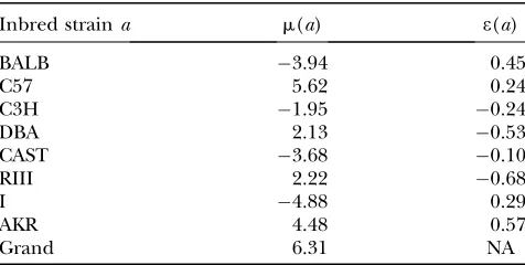
Note the absence here of a QTL variance contribution. Although the data are analyzed conditionally given observed marker genotypes, they are generated un-conditionally. Table 3 displays the values of the param-eters used for the simulations. These values were chosen randomly subject to constraints such asPamðaÞ ¼0.
Our simulation choices present both opportunities and challenges. For example, the fact that each strain is assigned a unique QTL allele suggests that even a simple F2cross between two strains would be adequate to map
the QTL. This advantage is tempered by the long genetic distances separating the QTL from the flanking markers,
by the smallness of the QTL effects, by the similarity of these effects in some strains, and by the discordance of the QTL effects and the polygenic means effects.
In using random effect models for QTL mapping, inclusion of polygenic background is usually a good idea. If polygenic background is present but ignored, then the only way of accounting for relative correlations is through the QTL component. When we analyze the current data omitting polygenic background, every single chromosome location in the linkage analysis achieves a P-value ,0.00001. Adding polygenic back-ground causesP-values to reach more reasonable levels, ranging from 0.0019 to 0.3835. Subjecting theP-values to the (FDR) procedure highlights the QTL and one neighboring point as significant (Benjaminiet al.2001).
Figure 4 plots the function log10(P-value) along the
chromosome; as earlier, theP-values reflect the likeli-hood ratio tests of the QTL component. The QTL is located at 30 cM from the origin between marker D2Mit323 at 23 cM and marker D2Mit37 at 42 cM.
We also used these data to illustrate the application of the QTL association model. As in our linkage analysis, omitting polygenic background leads to unrealistically
small P-values. Figure 4 plots the log10(P-value) for
the association analysis with the polygenic background. The association results are similar to the linkage results. The marker with the most significant result is D2Mit323, which is the marker nearest to the QTL. The FDR procedure singles out D2Mit323 as the only significant association.
Comparison of computation times between the two models illustrates the speed of the association analysis. The linkage model requires4 hr for calculation of the coefficient matrices for each pedigree and 20 hr to estimate the parameters for each of the 17 points. The association model requires1.5 hr for all calculations at each of the five markers.
DISCUSSION
In the hope of mapping QTL with small effects, geneticists are undertaking more ambitious crosses with multiple strains, multivariate traits, and dense marker sets. The random effects models developed here will enable a smooth transition to more sophisticated statistical analysis. The greatest strength of the models
Figure 3.—Trivariate analysis, four-way cross on chromosome 3, trivariate results peak over marker D3Mit25 and D3Mit86. These peaks are lower than those obtained with univariate and bi-variate analyses.
TABLE 2
Four-way cross: mean estimates for bivariate leptin analysis at D3Mit127
Lep-4 Lep-15 Mean effect Estimate SE Estimate SE B6/C3 0.1273 0.0616 0.1258 0.0638 B6/D2 0.1686 0.0599 0.1675 0.0632 C/C3 0.1812 0.0593 0.1198 0.0615 C/D2 0.1399 0.0615 0.0781 0.0646 Grand 0.0157 0.0346 0.0243 0.0362
SE, standard error.
TABLE 3
Eight-strain cross: simulation generating parameters
Inbred straina m(a) e(a)
BALB 3.94 0.45
C57 5.62 0.24
C3H 1.95 0.24
DBA 2.13 0.53
CAST 3.68 0.10
RIII 2.22 0.68
I 4.88 0.29
AKR 4.48 0.57
is their ability to capture polygenic background parsi-moniously. A second strength is their versatility in handling large pedigrees, large numbers of contribut-ing strains, and multivariate traits. While we have warned against importing ideas wholesale from the rest of statistical genetics, judicious adaptations are fully warranted. For example, since environment can be exquisitely controlled for inbred strain experiments, models of gene-by-environment interaction can be put to good use on the mean level (Blangero1993) and on
the variance level (Lange 1986; Itoh and Yamada
1990). These techniques apply both to continuous traits (Pletcher1999; Pletcherand Geyer1999; Jaffre´ ic
and Pletcher 2000; Pletcher and Jaffre´ ic 2002;
Purcell 2002; Purcell and Sham 2002; Meyer and
Kirkpatrick 2005) and to categorical traits (Towne et al.1997; Vielet al.2005). It is also straightforward to
model multiple QTL acting additively (Lange2002).
Balanced against these strengths is the need for better-conceived study designs. Unless crosses are care-fully structured, some parameters will be unidentifiable. One antidote is to scale back the complexity of a model and reparameterize. Our first two examples illustrate this tactic. Another antidote is to avoid monolithic designs and opt for a mixture of designs that individu-ally reveal different features of a model. Our third example does this.
In random effects models, trait values for most animals are correlated. Logically, one should treat all animals as members of a single large pedigree. At some point this requirement becomes unwieldy. The computational demands of the random effects models are fairly high, so tactics such as pedigree splitting, marker thinning, and marker amalgamation should not be dismissed. It will probably take a combination of these tactics to cope with the large-scale mapping projects now under way (Pletcher et al. 2004). Fortunately, our experiences
with simulated data suggest that a moderate amount of pedigree splitting sacrifices little information.
We have omitted a detailed discussion of how the program SimWalk delivers conditional strain fractions and coefficients. In our experience, SimWalk’s MCMC algorithm adequately samples descent graph space. In association analysis, this lengthy process can be dis-pensed with if information at neighboring markers is ignored. Deterministic algorithms that produce approx-imate kinship and strain coefficients may ultapprox-imately be a better choice than stochastic sampling (Gaoet al.2004;
Gao and Hoeschele 2005). In maximizing
loglikeli-hoods, it is also worth mentioning that Mendel allows the user to set initial parameter values and bounds. This flexibility is valuable in exploring multimodal likeli-hood surfaces.
Our QTL parameters enter the model at both the mean and the variance level and are not subject to nonnegativity constraints. Thus, the asymptotic distri-bution of a likelihood ratio test follows a chi-square distribution with degrees of freedom equal to the difference in the number of independent parameters between the underlying nested models. Model selection can be accomplished by likelihood ratio tests or mod-ified criteria such as the Akaike information criteria (AIC) or the Bayesian information criteria (BIC). Multiple testing is certainly an issue. The FDR correc-tion of Benjamini and Hochberg (Benjaminiet al.2001)
for dependent tests is often a useful cure and provided us with correct inferences in our simulated examples. Extensions such as Storey’s optimal discovery procedure (Storey 2007; Storey et al. 2007) can lead to more
accurateP-values and should be kept in mind.
The assumption of multivariate normality is helpful in maximum likelihood estimation. For univariate traits with excess kurtosis, the multivariatetdistribution is a workable substitute for the multivariate normal distri-bution and is an implemented option in Mendel. It is reasonable to conjecture that some version of the central limit theorem should hold for a polygenic trait
over a pedigree (Lange 1978; Lange and Boehnke
1983). For simple pedigrees generated en masse in a cross, one can check the normality assumption empir-ically. The impact of departures from normality has been considered by several researchers (Beaty et al.
1985; Allisonet al.1999; Prattet al.2000). Blangero et al.(2000) and Shamet al.(2000) suggest solutions to
gross violations. One can object that QTL effects by their discrete nature cannot be normal. Three responses are possible. First, this objection has never stopped ordinary QTL mapping with outbred populations. Second, under the null hypothesis, the discrete effects disappear. Third, in all but the simplest crosses, applica-tion of a rigorous model incorporating both polygenes and major genes is very computationally demanding.
The web site (http://www.genetics.ucla.edu/software) offers the current versions of Mendel and SimWalk for
several computing platforms. Ample documentation and sample problems are provided. The experimental versions of Mendel and SimWalk featured in this article will be released publicly as soon as it is practical.
The authors are grateful to David Burke for access to the UM-HET3 data, to Karl Broman for his editorial interest and guidance, and to the anonymous reviewers for their helpful comments. This investigation was supported by U.S. Public Health Service grants MH59490, GM53275, T32-HG02536, and HL28481.
LITERATURE CITED
Allison, D. B., M. C. Neale, R. Zannolli, N. J. Schork, C. I. Amos et al., 1999 Testing the robustness of the likelihood-ratio test in a variance-component quantitative-trait loci-mapping procedure. Am. J. Hum. Genet.65:531–544.
Amos, C. I., 1994 Robust variance-components approach for assess-ing genetic linkage in pedigrees. Am. J. Hum. Genet.54:535–543. Amos, C. I., M.deAndradeand D. K. Zhu, 2001 Comparison of multivariate tests for genetic linkage. Hum. Hered.51:133–144. Bauman, L. E., L. Almasy, J. Blangero, R. Duggirala, J. Sinsheimer et al., 2005 Fishing for pleiotropic QTLs in a polygenic sea. Ann. Hum. Genet.69:590–611.
Beaty, T. H., S. G. Self, K.-Y. Liang, M. A. Connolly, G. A. Chase et al., 1985 Use of robust covariance components models to an-alyse triglyceride data in families. Ann. Hum. Genet.49:315–328. Benjamini, Y., D. Drai, G. Elmer, N. Kafkafi and I. Golani, 2001 Controlling the false discovery rate in behavior genetics research. Behav. Brain Res.125:279–284.
Blangero, J., 1993 Statistical approaches to human adaptability. Hum. Biol.65:941–966.
Blangero, J., and L. Almasy, 1997 Multipoint oligogenic linkage analysis of quantitative traits. Genet. Epidemiol.14:959–964. Blangero, J., J. T. Williamsand L. Almasy, 2000 Robust lod scores
for variance component-based linkage analysis. Genet. Epide-miol.19:S8–S14.
Broman, K. W., H. Wu, S´. Senand G. A. Churchill, 2003 R/qtl: QTL mapping in experimental crosses. Bioinformatics 19:
889–890.
Cervino, A. C. L., A. Darvasi, M. Fallahi, C. C. Maderand N. F. Tsinoremas, 2007 An integratedin silicogene mapping strategy in inbred mice. Genetics175:321–333.
Churchill, G. A., and R. W. Doerge, 1994 Empirical threshold val-ues for quantitative trait mapping. Genetics138:963–971. Darvasi, A., and M. Soller, 1995 Advanced intercross lines, an
ex-perimental population for fine genetic mapping. Genetics141:
1199–1207.
Dawson, D. V., and R. C. Elston, 1984 A bivariate problem in human-genetics—ascertainment of families through a correlated trait. Am. J. Med. Genet.18:435–448.
Flint, J., W. Valdar, S. Shifmanand R. Mott, 2005 Strategies for mapping and cloning quantitative trait genes in rodents. Nat. Rev. Genet.6:271–286.
Gao, G., and I. Hoeschele, 2005 Approximating identity-by-descent matrices using multiple haplotype configurations on pedigrees. Genetics171:365–376.
Gao, G., I. Hoeschele, P. Sorensenand F. Du, 2004 Conditional probability methods for haplotyping in pedigrees. Genetics167:
2055–2065.
Goldgar, D. E., 1990 Multipoint analysis of human quantitative genetic-variation. Am. J. Hum. Genet.47:957–967.
Haley, C. S., and S. A. Knott, 1992 A simple regression method for mapping quantitative trait loci in line crosses using flanking markers. Heredity69:315–324.
Harper, J. M., A. T. Galecki, D. T. Burke, S. L. Pinkoskyand R. A. Miller, 2003 Quantitative trait loci for insulin-like growth fac-tor I, leptin, thyroxine, and corticosterone in genetically hetero-geneous mice. Physiol. Genomics15:44–51.
Hitzemann, R. W., B. Malmanger, S. Cooper, S. Coulombe, C. Reed et al., 2002 Multiple cross mapping (MCM) markedly improves the localization of a QTL for ethanol-induced activation. Genes Brain Behav.1:214–222.
Hopper, J. L., and J. D. Mathews, 1982 Extensions to multivariate nor-mal models for pedigree analysis. Ann. Hum. Genet.46:373–383. Itoh, Y., and Y. Yamada, 1990 Relationships between genotype x en-vironment interaction and genetic correlation of the same trait measured in different environments. Theor. Appl. Genet.80:11–16. Jaffre´ ic, F., and S. D. Pletcher, 2000 Statistical models for estimat-ing the genetic basis of repeated measures and other function-valued traits. Genetics156:913–922.
Janninka, J.-L., and R. Jansena, 2001 Mapping epistatic quantitative trait loci with one-dimensional genome searches. Genetics157:
445–454.
Kao, C.-H., Z.-B. Zengand R. D. Teasdale, 1999 Multiple interval mapping for quantitative trait loci. Genetics152:1203–1216. Kruglyak, L., M. J. Daly, M. P. Reeve-Daly and E. S. Lander,
1996 Parametric and nonparametric linkage analysis: a unified multipoint approach. Am. J. Hum. Genet.58:1347–1363. Lander, E. S., and D. Botstein, 1989 Mapping Mendelian factors
underlying quantitative traits using RFLP linkage maps. Genetics
121:185–199.
Lange, K., 1978 Central limit theorems for pedigrees. J. Math. Biol.
6:59–66.
Lange, K., 1986 Cohabitation, convergence and environmental co-variances. Am. J. Med. Genet.24:483–491.
Lange, K., 2002 Mathematical and Statistical Methods for Genetic Anal-ysis, Ed. 2. Springer-Verlag, New York.
Lange, K., and M. Boehnke, 1983 Extensions to pedigree analysis. IV. Covariance components models for multivariate traits. Am. J. Med. Genet.14:513–524.
Lange, K., J. S. Sinsheimerand E. M. Sobel, 2005 Association test-ing with Mendel. Genet. Epidemiol.29:36–50.
Li, R., M. A. Lyons, H. Wittenburg, B. Piagenand G. A. Churchill, 2005 Combining data from multiple inbred line crosses im-proves the power and resolution of quantitative trait loci map-ping. Genetics169:1699–1709.
Liu, Y., and Z.-B. Zeng, 2000 A general mixture model approach for mapping quantitative trait loci from diverse cross designs involv-ing multiple inbred lines. Genet. Res.75:345–355.
Manly, K. F., and J. M. Olson, 1999 Overview of QTL mapping soft-ware and introduction to Map Manager QT. Mamm. Genome10:
327–334.
Meyer, K., and M. Kirkpatrick, 2005 Up hill, down dale: quantita-tive genetics of curvaceous traits. Philos. Trans. R. Soc.360:1443– 1455.
Mott, R., C. J. Talbot, M. G. Turri, A. C. Collinsand J. Flint, 2000 A method for fine mapping quantitative trait loci in out-bred animal stocks. Proc. Natl. Acad. Sci. USA97:12649–12654. Pletcher, M. T., P. McClurg, S. Batalov, A. I. Su, S. W. Barneset al., 2004 Use of a dense single nucleotide polymorphism map for in silico mapping in the mouse. PLoS Biol.2:2159–2169. Pletcher, S. D., 1999 Model fitting and hypothesis testing for
age-specific mortality data. J. Evol. Biol.12:430–439.
Pletcher, S. D., and C. J. Geyer, 1999 The genetic analysis of age-dependent traits: modeling the character process. Genetics153:
825–835.
Pletcher, S. D., and F. Jaffre´ ic, 2002 Generalized character pro-cess models: estimating the genetic basis of traits that cannot be observed and that change with age or environmental condi-tions. Biometrics58:157–162.
Pratt, S. C., M. J. Dalyand L. Kruglyak, 2000 Exact multipoint quantitative-trait linkage analysis in pedigrees by variance compo-nents. Am. J. Hum. Genet.6:1153–1157.
Purcell, S., 2002 Variance components models for gene-environ-ment interaction in twin analysis. Twin Res.5:554–571. Purcell, S., and P. Sham, 2002 Variance components models for
gene-environment interaction in quantitative trait locus linkage analysis. Twin Res.5:572–576.
Rebai, A., and B. Goffinet, 1993 Power of tests for QTL detection using replicated progenies derived from a diallel cross. Theor. Appl. Genet.86:1014–1022.
Schork, N. J., 1993 Extended multipoint identity-by-descent analy-sis of human quantitative traits: efficiency, power, and modeling considerations. Am. J. Hum. Genet.53:1306–1319.
Sen, S´., and G. A. Churchill, 2001 A statistical framework for quan-titative trait mapping. Genetics159:371–387.
Sham, P. C., J. H. Zhao, S. S. Chernyand J. K. Hewitt, 2000 Variance-components QTL linkage analysis of selected and non-normal samples: conditioning on trait values. Genet. Epidemiol.19:S22– S28.
Sillanpa¨ a¨, M. J., and E. Arjas, 1998 Bayesian mapping of multiple quantitative trait loci from incomplete inbred line cross data. Ge-netics148:1373–1388.
Sobel, E. M., and K. Lange, 1996 Descent graphs in pedigree anal-ysis: applications to haplotyping, location scores, and marker-sharing statistics. Am. J. Hum. Genet.58:1323–1337.
Storey, J. D., 2007 The optimal discovery procedure: a new ap-proach to simultaneous significance testing. J. R. Stat. Soc. B
69:347–368.
Storey, J. D., J. Y. Daiand J. T. Leek, 2007 The optimal discovery procedure for large-scale significance testing, with applications to comparative microarray experiments. Biostatistics8:414–432. Towne, B., R. M. Siervogeland J. Blangero, 1997 Effects of geno-type-by-sex interaction on quantitative trait linkage analysis. Genet. Epidemiol.14:1053–1058.
Valdar, W., J. Flintand R. Mott, 2006 Simulating the collabora-tive cross: power of quantitacollabora-tive trait loci detection and mapping
resolution in large sets of recombinant inbred strains of mice. Genetics172:1783–1797.
Viel, K. R., D. M. Warren, A. Buil, T. D. Dyer, T. E. Howardet al., 2005 A comparison of discrete versus continuous environment in a variance components-based linkage analysis of the COGA data. BMC Genet.6(Suppl. 1): S57.
Williams, R. W., K. W. Broman, J. M. Cheverud, G. A. Churchill, R. W. Hitzemannet al., 2002 A collaborative cross for high-precision complex trait analysis. First workshop report of the complex trait consortium. Technical report.
Xie, C., D. D. G. Gesslerand S. Xu, 1989 Combining different line crosses for mapping quantitative trait loci using the identical by descent-based variance component method. Genetics149:1139– 1146.
Zeng, Z.-B., 1993 Theoretical basis for separation of multiple linked gene effects in mapping quantitative trait loci. Proc. Natl. Acad. Sci. USA90:10972–10976.
Zeng, Z.-B., 1994 Precision mapping of quantitative trait loci. Ge-netics136:1457–1468.
Communicating editor: K. W. Broman
APPENDIX A: REPRESENTATION OF POSITIVE DEFINITE MATRICES
Given ak3kpositive definite matrixVand ak31 vectorm, we now prove that vectorsm1,. . .,mnexist such that
P
imi¼mand
P
imimi*¼V. To simplify the proof, we pass to the spectral decompositionV¼O*DOofV. HereOis an
orthogonal matrix, andDis a diagonal matrix whosejth diagonal entrydjis an eigenvalue ofV. Ifnvectorsn1,. . .,nn
exist such thatPini ¼Om¼nandPinin*i ¼D, then takingmi¼O*nifor eachicompletes the proof.
With the transformed problem, we can work on each dimensionjseparately. Suppose we can find scalarsa1,. . .,am
such thata11. . .1am¼njanda121. . .1a2m¼dj. Then we constructmvectorsw1,. . .,wmwhose entries are 0 except
for theirjth entrieswij¼ai. Thesemvectors compose part of the solution setn1,. . .,nnand do not impinge on the parts
contributed by other dimensions. To show that appropriate scalars a1,. . ., am exist, we consider optimizing the functionf(a)¼a2
11. . .1a
2
msubject to the affine constrainta11. . .1am¼nj. By introducing a Lagrange multiplier,
we can prove thatf(a) attains its minimumn2
j=mwhen allai¼nj/m. The maximum off(a) is infinite in all but the trivial
casem¼1. For instance, we can takea1¼1
2ðnj1pÞ,a2¼12ðnjpÞ, and all otherai¼0 and sendpto‘. Sincedjmust be
positive, some positive integermexists withn2
j=m,dj. This choice ofmputs us in a position to invoke the intermediate
value theorem. The set of vectorsa¼(a1,. . .,am) satisfying the constraint is convex and therefore connected. A continuous function on a connected set attains every value between its minimum and maximum values. Hence, there is someawithf(a)¼dj.
APPENDIX B: PROPERTIES OF THECijMATRICES
The role of the matrixCijin formula (3) suggests its importance. MathematicallyCijis better behaved than the strain coefficient matrixcij. Recall that the founder initial conditions and the recurrences (4)–(7) completely determine the
strain fraction vectorsgiand the strain coefficient matricescij. If we retain the conventions thatihas parentskandl
andjis an animal previously considered, then the last three recurrences translate into the similar recurrences
Cij ¼cijgigj*
¼1
2ðckj1cljÞ 1
2ðgk1glÞgj* ¼1
2ðCkj1CljÞ ðB1Þ
Cji¼
1
2ðCjk1CjlÞ ðB2Þ
Cii¼ciigigi*
¼1
4½diagðgkÞ1diagðglÞ1gkgl*1glgk*
1
4ðgk1glÞðgk1glÞ* ¼1
4½diagðgkÞ1diagðglÞ gkgk*glgl* ðB3Þ
on theCijmatrices. The next proposition collects some relevant facts.
Proposition1.In addition to satisfying the recurrences(B1), (B2),and(B3),the matrix Cij
a. has all entries0when either i or j is a founder, b. is symmetric,
c. is positive semidefinite,
d. has the vector1in its null space,
e. has entries Cij(m,n)confined to the interval½1
8;0for n6¼m and to the interval½0; 1
8for n¼m. Proof.
a. Ifiis a founder belonging to strainqandjis a founder belonging to strainr, then by definitiongi(m)¼1{m¼q},gj(n)¼
1{n¼r}, andcij(m,n)¼1{m¼q}1{n¼r}. Thus, all entries ofCijvanish. Ifiorjis a founder but the other is not, then
induction and the recurrences (B1) and (B2) show that all entries ofCijvanish.
b. Formula (B3) forcesCiito be symmetric, and the recurrences (B1) and (B2) preserve symmetry.
c. Because the recurrences (B1) and (B2) preserve positive semidefiniteness, it suffices to prove thatCiiis positive semidefinite. Inspection of formula (B3) further demonstrates that it suffices to prove that diag(gk)gkgk* is
positive semidefinite for allk. Accordingly, letvbe an arbitrary vector. The quadratic form
v* diagð½ gkÞ gkgk*v¼X
m
gkðmÞvm2 X
m
gkðmÞvm
" #2
is nonnegative owing to Cauchy’s inequality
X
m
gkðmÞvm
" #2
# X
m
gkðmÞ
" #
X
m
gkðmÞvm2
" #
and the fact thatPmgkðmÞ ¼1.
d. Again this is a consequence of the recurrences (B1) and (B2) and the validity of the assertion forCii. In the latter case, the equality
diagðgkÞ gkgk*
½ 1¼gkgkgk*1¼0
is obvious.
e. Because the stated bounds are preserved by recurrences (B1) and (B2), it suffices to considerCii. The contribution
1
4gkðmÞ½1gkðmÞto a diagonal term in Equation B3 is bounded below by 0 and above by161. The contribution
1
4gkðmÞgkðnÞto an off-diagonal term is bounded below by161 and above by 0. n
The collectionCof allCijmatrices over a pedigree has considerable structure. For example, the symmetry of Cij
entailsCij¼Cji. With justs¼2 strains, parts b, d, and e of Proposition 1 imply that everyCijis representable as
Cij¼aij
1 1
1 1
for some constantaij 2 ½0;1
8. Furthermore, sinceaij¼0 wheneveriorjis a founder or an F1individual, straightforward
recursive arguments show that within any strictly linear mating designs like Fn,aij¼0 for alli6¼j. Two-strain systems also
produce uninterestingconditionalcoefficients; straightforward calculations show thatCiˆj ¼0for alliandjat markers
that differentiate between the strains with complete genotyping.
To generalize this representation to more than two strains, it is helpful to introduce thes3smatrixEmnwhere all entries ofEmnare 0 except foremm¼enn¼1 andemn¼enm¼ 1. There areðs