ABSTRACT
SMITH, LUKE BRAWLEY. Bayesian Quantile Regression in Biostatistical Applications. (Under the direction of Montserrat Fuentes and Brian Reich.)
Quantile regression offers a useful alternative to mean regression when researchers are inter-ested in noncentral aspects of the distribution. In this dissertation we extend quantile regression
methods inside of a multilevel Bayesian framework to accommodate temporal correlation,
flexi-ble tails, discrete data, mixed regression effects and multivariate response. These methodological advances are motivated by and illustrated with two biostatistical applications: a study of air
pol-lution effects on birth outcomes in Texas and a study of urbanization effects on blood pressure
in China.
Infants born preterm or small for gestational age have elevated rates of morbidity and
mor-tality. Utilizing birth certificate records in Texas from 2002-2004 and Environmental Protection
Agency air pollution estimates, we relate the quantile functions of birth weight and gestational age to ozone exposure and multiple predictors, including parental age, race, and education level.
We introduce a semi-parametric Bayesian quantile model that collectively estimates the
rela-tionship between the predictors and birth weight for multiple gestational ages, provides more flexibility in the tails than previous quantile function approaches, and to our knowledge is the
first quantile function model to accommodate discrete response. Our multilevel quantile
func-tion model establishes relafunc-tionships between birth weight and the predictors separately for each week of gestational age and between gestational age and the predictors separately across Texas
Public Health Regions. We permit these relationships to vary nonlinearly across gestational
age, spatial domain and quantile level and we unite them in a hierarchical model via a basis expansion on the regression coefficients that preserves interpretability. Very low birth weight is
a primary concern, so we leverage extreme value theory to enhance flexibility in the tail of the
distribution. Gestational ages are rounded into weekly values, so we present methodology for modeling quantile functions of discrete response data. In a simulation study we show that
pool-ing information across gestational age and quantile level substantially reduces MSE of predictor
effects relative to standard frequentist quantile regression. We find that ozone is negatively as-sociated with the lower tail of gestational age in south Texas and across the distribution of
birth weight for high gestational ages. Our methods are available in the R packageBSquare. The second application we consider is blood pressure in China. Cardiometabolic risk has
substantially increased in China in the past 20 years and blood pressure is a primary
modi-fiable risk factor. Using data from the China Health and Nutrition Survey we examine blood pressure trends in China from 1991 to 2009, with a concentration on age cohorts and
functions of systolic and diastolic blood pressure. This allows the covariate effects in the middle
of the distribution to vary from those in the upper tail, the focal point of our analysis. We join the distributions of systolic and diastolic blood pressure using a copula, which permits the
relationships between the covariates and the two responses to share information and enables
probabilistic statements about systolic and diastolic blood pressure jointly. Our copula main-tains the marginal distributions of the group quantile effects while accounting for within-subject
dependence, enabling inference at the population and subject levels. We present a multilevel
framework that enables straightforward hypothesis testing for changes in covariate effects across time. Our population level regression effects change across quantile level, year, and blood
pres-sure type, providing a rich environment for inference. To our knowledge, this is the first quantile
function model to explicitly model within-subject autocorrelation and is the first quantile func-tion model that accommodates multivariate response. We find that the associafunc-tion between
high blood pressure and living in an urban area has evolved from positive to negative, with the
strongest changes occurring in the upper tail.
A major challenge in large-scale epidemiological studies such as those described above is
accurate quantification of the exposure of interest. In the final chapter we develop a spatial
model to improve estimates of ambient air pollution exposure. We examine three pollutants, total fine particulate matter and two of its components, nitrate and sulfate. We compare
in-dividually constructed pollutant surfaces to a multivariate regression model undergirded with one spatial surface. We investigate the spatial and temporal bias of the US Environmental
Pro-tection Agency’s Community Multi-scale Air Quality model. We find that the spatial signal in
©Copyright 2014 by Luke Brawley Smith
Bayesian Quantile Regression in Biostatistical Applications
by
Luke Brawley Smith
A dissertation submitted to the Graduate Faculty of North Carolina State University
in partial fulfillment of the requirements for the Degree of
Doctor of Philosophy
Statistics
Raleigh, North Carolina
2014
APPROVED BY:
Yang Zhang Yichao Wu
Montserrat Fuentes Co-chair of Advisory Committee
Brian Reich
DEDICATION
This thesis would not be possible without the love and support of the most important people in my life. To Merissa, my best friend. To Mom and Dad, for always being in my corner and
BIOGRAPHY
The author grew up in lovely Washington state, graduating from Western Washington Univer-sity in 2002 with a degree in English literature. Since then, the author has taught English in
ACKNOWLEDGEMENTS
I thank Montse and Brian for their tremendous investment and positive energy. I thank commit-tee members Yang Zhang, Yichao Wu, and Judy Wang for their service. I thank Amy Herring
for her collaboration and guidance. I thank Chris Waddell for teaching me the C computing lan-guage and his help learning GPUs. I thank collaborators Brian Eder and Penny Gordon-Larsen
TABLE OF CONTENTS
LIST OF TABLES . . . vii
LIST OF FIGURES . . . .viii
Chapter 1 Introduction . . . 1
1.1 Quantile Regression . . . 1
1.2 Copulas . . . 3
Chapter 2 Multilevel Quantile Function Modeling with Application to Birth Outcomes . . . 5
2.1 Introduction . . . 5
2.2 Methods . . . 9
2.2.1 Individual Quantile Function . . . 9
2.2.2 Multilevel Quantile Model . . . 11
2.2.3 Tail Modeling . . . 12
2.2.4 Discrete Data . . . 14
2.2.5 Computation . . . 14
2.3 Simulation Study . . . 15
2.4 Birth Outcome Analyses . . . 18
2.4.1 Data Description . . . 18
2.4.2 Gestational Age Personal Characteristic Results . . . 18
2.4.3 Birth Weight Personal Characteristic Results . . . 20
2.4.4 Ozone Results . . . 21
2.5 Conclusions . . . 22
Chapter 3 Quantile Regression for Mixed Models . . . 25
3.1 Introduction . . . 25
3.2 Methods . . . 27
3.2.1 Marginal Quantile Model . . . 27
3.2.2 Mixed Effects Quantile Model . . . 28
3.2.3 Multivariate Mixed Effects Quantile Model . . . 30
3.3 Simulation Study . . . 31
3.4 CHNS Analysis . . . 32
3.4.1 Data . . . 32
3.4.2 Analysis . . . 35
3.5 Conclusions . . . 40
Chapter 4 Prediction of Speciated Particulate Matter and Bias Assessment of Numerical Output Data . . . 43
4.1 Introduction . . . 43
4.2 Materials and Methods . . . 45
4.2.1 Data Description . . . 45
4.2.3 Spatiotemporal Model . . . 47
4.2.4 Multivariate Model . . . 48
4.3 Results . . . 49
4.3.1 Prediction . . . 49
4.3.2 Bias . . . 52
4.4 Conclusions . . . 55
References. . . 56
Appendices . . . 65
Appendix A . . . 66
A.1 Chapter 2 MCMC Details . . . 66
A.2 Chapter 2 Supplementary Materials . . . 66
Appendix B . . . 110
B.1 Chapter 3 MCMC Details . . . 110
B.1.1 Quantile Parameters . . . 110
B.1.2 Copula Parameters . . . 111
LIST OF TABLES
Table 2.1 Log pseudo marginal likelihood (LPML) of model fits for the birth outcomes, with higher values corresponding to better fits. Minimum values for gestational age (-1,077,185) and birth weight (-4,094,739) were subtracted from the values shown below for clarity. Model types include exponential tail (Exp), Pareto tail with shape constant for all Public Health Regions or gestational ages (Par), shape changing across Public Health Region or gestational age (Change), and independent models for each Public Health Region and gestational age (Ind). Bolded values signify the best fit. . . 24
Table 3.1 Coverage probability (CP) and mean squared error (MSE) for the N = 50
arm of the simulation study. Nominal coverage probability is 95%. We compare treating the data as independent within a subject (“Ind”), fitting with a copula (“Cop”), and the random effects model of (Reich et al., 2010a) (“RBW”). Coverage and MSE were evaluated at and averaged over the quantile levels
{0.1,0.3,0.5,0.7,0.9}. For datatype = 1, MSE values are less than depicted values by a factor of 10. Estimators whose MSE were statistically significantly different than the copula model are indicated by ∗. . . 41 Table 3.2 Posterior parameter estimates and 95% credible intervals for location effects.
Mean effects include age cohort (with baseline group aged 40-50), urbanization by age cohort interaction (indicated by U *), household income (HHI), current pregnancy status, and smoking. . . 42
Table 4.1 Monitor means and standard deviations of total PM2.5, nitrate, and sulfate
inµg/m3, going from winter (top row) to fall (bottom row). . . 49 Table 4.2 Cross validation mean absolute deviation (MAD), coverage of 95% intervals
(CP) and predictive R-squared (R2) for the full model (Full), kriging with
CMAQ (K-CMAQ) and without (K-NoCMAQ), as well as the multivariate model (Multi). Standard errors for PM2.5 MAD did not exceed 0.09 and
stan-dard errors for nitrate and sulfate MAD were all below 0.03. Paired t-tests revealed statistically significant differences for MAD comparisons between the full and kriging with CMAQ models excepting autumnal sulfate. . . 50
LIST OF FIGURES
Figure 2.1 Boxplots of birth weight by week of gestational age. . . 7 Figure 2.2 Texas Public Health Regions. . . 8 Figure 2.3 MSE Ratios of quantile function estimator over frequentist quantile estimator
and coverage probabilities. The maximum Monte Carlo standard error of MSE was 0.35 for Bayesian estimators and 1.2 for the frequentist estimator. The maximum Monte Carlo standard error for the MSE ratio was 0.53 at
τ = 0.01 and 0.13 for other quantile levels. . . 17 Figure 2.4 95% credible limits for the posterior distribution of the difference in
gesta-tional age between black non-Hispanic and white non-Hispanic mothers by Public Health Region (PHR). . . 19 Figure 2.5 95% credible limits for the posterior distribution of the effect of a one-unit
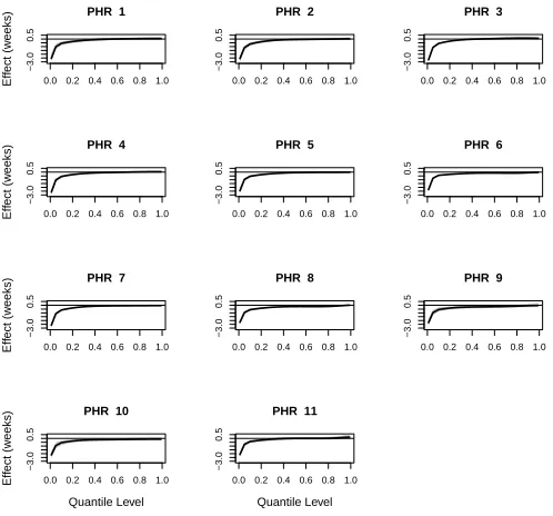
increase in second trimester ozone exposure on gestational age by Public Health Region. All ozone values were linearly transformed into [-1,1], so a one-unit increase can be roughly thought of as an increase from low levels to middle levels of exposure, or middle to high. . . 21 Figure 2.6 95% credible limits for the posterior distribution of the effect of a one-unit
increase in second trimester ozone exposure on birth weight for gestational age of 34-42 weeks. All ozone values were linearly transformed into [-1,1], so a one-unit increase can be roughly thought of as an increase from low levels to middle levels of exposure, or middle to high. Light gray regions correspond to posterior credible sets for individual fits at each gestational age while dark gray regions correspond to the collective fit across gestational age. Dashed lines indicate limits of 95% frequentist confidence intervals. . . 23
Figure 3.1 Systolic blood pressure (SBP) and diastolic blood pressure (DBP) by gender and urbanization scores across time. Blood pressure measurements are in mil-limeters of mercury (mmHg) while urbanization measurements are unitless. Horizontal lines represent thresholds for high blood pressure, located at 140 mmHg and 90 mmHg for systolic and diastolic blood pressure respectively. . 34 Figure 3.2 Plots of posterior credible sets of urbanization random effects on females for
systolic blood pressure. For visual clarity posterior credible sets are ordered by posterior median and every 10th subject is shown. . . 36 Figure 3.3 Plots of the 2009 urbanization effects by gender and blood pressure type.
Dark regions correspond to individual fits, while light regions correspond to simultaneous estimates. . . 38 Figure 3.4 Plots of the intercept process for the age 40-50 cohort and population
urban-ization effects by gender and blood pressure type. Dark regions correspond to 1991 estimates, while light regions correspond to 2009 estimates. . . 39
Figure 4.2 Posterior means of additive (αt) and multiplicative (βt) biases. Intercept
standard deviations were around 1 for PM and smaller for other pollutants.
Slope standard deviations were less than 0.2. . . 52
Figure 4.3 Additive biases by season for PM2.5 inµg/m3. . . 53
Figure 4.4 Additive biases by season for nitrate in µg/m3. . . 54
Figure 4.5 Additive biases by season for sulfate in µg/m3. . . 54
Figure A.1 MSE ratios of quantile function estimator over frequentist quantile estimator and coverage probabilities for beta quantile functions. The maximum Monte Carlo standard error of MSE was 0.2 for Bayesian estimators and 0.3 for the frequentist estimator. The maximum Monte Carlo standard error for the MSE ratio was 0.09. . . 67
Figure A.2 95% credible limits for the posterior distribution of the intercept process for gestational age by Public Health Region (PHR). The intercept process represents the information regarding gestational age not explained by the predictors and was permitted to vary by PHR. The intercept process is not interpretable, as we had binary variables that were valued at either -1 or 1. . 68
Figure A.3 95% credible limits for the posterior distribution of the effect of being male vs. female on gestational age by Public Health Region (PHR). . . 69
Figure A.4 95% credible limits for the posterior distribution of the effect of maternal parity on gestational age by Public Health Region (PHR). . . 70
Figure A.5 95% credible limits for the posterior distribution of the effect of maternal age 40 and above on gestational age by Public Health Region (PHR). . . 71
Figure A.6 95% credible limits for the posterior distribution of the effect of paternal age 40 and above on gestational age by Public Health Region (PHR). . . 72
Figure A.7 95% credible limits for the posterior distribution of the effect of the mother finishing high school relative to not finishing high school on gestational age by Public Health Region (PHR). . . 73
Figure A.8 95% credible limits for the posterior distribution of the effect of the mother finishing education above high school relative to not finishing high school on gestational age by Public Health Region (PHR). . . 74
Figure A.9 95% credible limits for the posterior distribution of the effect of the father finishing high school relative to not finishing high school on gestational age by Public Health Region (PHR). . . 75
Figure A.10 95% credible limits for the posterior distribution of the effect of the father finishing education above high school relative to not finishing high school on gestational age by Public Health Region (PHR). . . 76
Figure A.11 95% credible limits for the posterior distribution of the effect of black non-Hispanic maternal ethnicity relative to white non-non-Hispanic maternal ethnicity on gestational age by Public Health Region (PHR). . . 77
Figure A.13 95% credible limits for the posterior distribution of the effect of other mater-nal ethnicity relative to white non-Hispanic matermater-nal ethnicity on gestatiomater-nal age by Public Health Region (PHR). . . 79 Figure A.14 95% credible limits for the posterior distribution of the effect of a one-unit
increase in first trimester ozone exposure on gestational age by Public Health Region (PHR). All ozone values were linearly transformed into [-1,1], so a one-unit increase can be roughly thought of as an increase from low levels to middle levels of exposure, or middle to high. . . 80 Figure A.15 95% credible limits for the posterior distribution of the effect of a one-unit
increase in second trimester ozone exposure on gestational age by Public Health Region (PHR). All ozone values were linearly transformed into [-1,1], so a one-unit increase can be roughly thought of as an increase from low levels to middle levels of exposure, or middle to high. . . 81 Figure A.16 95% credible limits for the posterior distribution of the intercept of birth
weight for gestational ages 25-33 weeks. . . 82 Figure A.17 95% credible limits for the posterior distribution of the intercept of birth
weight for gestational ages 34-42 weeks. . . 83 Figure A.18 95% credible limits for the posterior distribution of the effect of male sex
relative to female on birth weight for gestational ages 25-33 weeks. . . 84 Figure A.19 95% credible limits for the posterior distribution of the effect of male sex
relative to female on birth weight for gestational ages 34-42 weeks. . . 85 Figure A.20 95% credible limits for the posterior distribution of the effect of maternal
parity on birth weight for gestational ages 25-33 weeks. . . 86 Figure A.21 95% credible limits for the posterior distribution of the effect of maternal
parity on birth weight for gestational ages 34-42 weeks. . . 87 Figure A.22 95% credible limits for the posterior distribution of the effect of maternal
age greater than 40 relative to maternal age less than 40 on birth weight for gestational ages 25-33 weeks. . . 88 Figure A.23 95% credible limits for the posterior distribution of the effect of maternal
age greater than 40 relative to maternal age less than 40 on birth weight for gestational ages 34-42 weeks. . . 89 Figure A.24 95% credible limits for the posterior distribution of the effect of paternal
age greater than 40 relative to paternal age less than 40 on birth weight for gestational ages 25-33 weeks. . . 90 Figure A.25 95% credible limits for the posterior distribution of the effect of paternal
age greater than 40 relative to paternal age less than 40 on birth weight for gestational ages 34-42 weeks. . . 91 Figure A.26 95% credible limits for the posterior distribution of the effect of the mother
finishing high school relative to not finishing high school on birth weight for gestational ages 25-33 weeks. . . 92 Figure A.27 95% credible limits for the posterior distribution of the effect of the mother
Figure A.28 95% credible limits for the posterior distribution of the effect of the mother finishing education above high school relative to not finishing high school on birth weight for gestational ages 25-33 weeks. . . 94 Figure A.29 95% credible limits for the posterior distribution of the effect of the mother
finishing education above high school relative to not finishing high school on birth weight for gestational ages 34-42 weeks. . . 95 Figure A.30 95% credible limits for the posterior distribution of the effect of the father
finishing high school relative to not finishing high school on birth weight for gestational ages 25-33 weeks. . . 96 Figure A.31 95% credible limits for the posterior distribution of the effect of the father
finishing high school relative to not finishing high school on birth weight for gestational ages 34-42 weeks. . . 97 Figure A.32 95% credible limits for the posterior distribution of the effect of the father
finishing education above high school relative to not finishing high school on birth weight for gestational ages 25-33 weeks. . . 98 Figure A.33 95% credible limits for the posterior distribution of the effect of the father
finishing education above high school relative to not finishing high school on birth weight for gestational ages 34-42 weeks. . . 99 Figure A.34 95% credible limits for the posterior distribution of the effect of maternal
black non-Hispanic ethnicity relative to white non-Hispanic ethnicity on birth weight for gestational ages 25-33 weeks. . . 100 Figure A.35 95% credible limits for the posterior distribution of the effect of maternal
black non-Hispanic ethnicity relative to white non-Hispanic ethnicity on birth weight for gestational ages 34-42 weeks. . . 101 Figure A.36 95% credible limits for the posterior distribution of the effect of maternal
Hispanic ethnicity relative to white non-Hispanic ethnicity on birth weight for gestational ages 25-33 weeks. . . 102 Figure A.37 95% credible limits for the posterior distribution of the effect of maternal
Hispanic ethnicity relative to white non-Hispanic ethnicity on birth weight for gestational ages 34-42 weeks. . . 103 Figure A.38 95% credible limits for the posterior distribution of the effect of maternal
other ethnicity relative to white non-Hispanic ethnicity on birth weight for gestational ages 25-33 weeks. . . 104 Figure A.39 95% credible limits for the posterior distribution of the effect of maternal
other ethnicity relative to white non-Hispanic ethnicity on birth weight for gestational ages 34-42 weeks. . . 105 Figure A.40 95% credible limits for the posterior distribution of the effect of a one unit
Figure A.41 95% credible limits for the posterior distribution of the effect of a one unit increase in first trimester ozone exposure on birth weight for gestational ages 34-42 weeks. All ozone values were linearly transformed into [-1,1], so a one-unit increase can be roughly thought of as an increase from low levels to middle levels of exposure, or middle to high. . . 107 Figure A.42 95% credible limits for the posterior distribution of the effect of a one unit
increase in second trimester ozone exposure on birth weight for gestational ages 25-33 weeks. All ozone values were linearly transformed into [-1,1], so a one-unit increase can be roughly thought of as an increase from low levels to middle levels of exposure, or middle to high. . . 108 Figure A.43 95% credible limits for the posterior distribution of the effect of a one unit
Chapter 1
Introduction
In Chapter 1 we introduce background concepts for the next chapters. In Section 1.1 we present the rudiments of quantile regression. We extend quantile regression methods in Chapters 2 and
3. In Section 1.2 we introduce copulas, which are utilized in Chapter 3.
1.1
Quantile Regression
The preponderance of statistical science has been directed at better estimating the mean of
a distribution. Denote Yi as the scalar response indexed by unit i, and let Xi be a vector of
covariates of lengthP. The classical mean regression model is
Yi =f(Xi,β) +Ei (1.1)
where β is a vector of regression coefficients, Ei iid
∼ F, and F is a distribution function with
mean zero. The conditional mean ofYi given Xi isf(Xi,β).
The most common form of (1.1) is linear regression, wheref(Xi,β) =X0iβ. Linear mean re-gression has many desirable attributes that make it the default for conditional inference. Means
are easy to conceptualize and give a reference point for the central tendency of a distribution. The regression coefficients are simple to interpret, as a one-unit increase in Xp is associated
with a βp increase in the conditional mean of the response. The solution to linear regression
is obtained by solving for β in the normal equation X0Y = X0Xβ with respect to squared error loss (SEL), the optimal loss function when estimating a conditional mean. Under the
Gauss-Markov assumptions, the closed-form solution to the normal equations is the best linear
unbiased estimator of the true regression coefficients with respect to SEL.
Despite these nice attributes, quantile regression (Koenker, 2005) is more suitable than mean
estimates under SEL. In some cases researchers are more interested in the impact of a covariate
on noncentral parts of the distribution. For inference the error distribution F in (1.1) is usually assumed to be Gaussian, which may be inappropriate. Quantile regression provides a useful
alternative in these scenarios.
Denote τ ∈ (0,1) as the quantile level and the τth quantile of a distribution F as the value Q(τ) where P(Yi ≤Q(τ)) =τ. The classical quantile regression model extends (1.1) by
defining Q(Xi,βτ) as the τth conditional quantile ofYi given Xi. Define the function ρτ(u) =
u(τ −1(u < 0)) as the check loss function. Just as the solution to the normal equations is
optimal with respect to SEL, theτthconditional quantile ofYi givenXi is optimal under check
loss. Therefore theτth conditional quantile of Yi given Xi is found by solving
min
βτ X
ρτ(Yi−Q(Xi,βτ)). (1.2)
Once again, the most common case of quantile regression is linear quantile regression, where
Q(Xi,βτ) =X0iβτ. Linear quantile regression has many nice properties, including interpretabil-ity. A one-unit increase in Xp is associated with aβp increase in the conditionalτth quantile of
the response. Assuming this linear form, the solution to (1.2) can be found via linear
program-ming and (1.2) is consistent under mild conditions. Quantiles are invariant under transformation (i.e. for monotonic nondecreasing function h,Q(h(Y)) =h(Q(Y)) ). Linear quantile regression
is invariant to equivariance of the design matrix ( ˆβ(τ;y;XA) =A−1βˆ(τ;y;X)). These final two
properties properties do not hold under the mean except under affine transformation (Koenker, 2005).
Yu and Moyeed (2001) introduced quantile regression in a Bayesian framework.
Minimiza-tion of (1.2) is equivalent to maximizaMinimiza-tion of the likelihood of the asymmetric Laplace distri-bution. The asymmetric Laplace distribution has location parameterµ and scale parameterσ,
with density
fτ(u;µ, σ) =
τ(1−τ)
σ exp
−ρτ
u−µ
σ
.
Lettingµ=Q(Xi,βτ) allows the covariates to affect the τth quantile of the response.
Researchers are often interested in conducting inference at multiple quantiles. The methods
above fit separate models for each quantile level. In applications where effects at proximate quantiles are expected to be similar, it is useful to borrow information across fits. In addition,
multiple fits can cause “crossing quantiles”, where at certain values of the covariates the
condi-tional quantile function is decreasing in quantile level (Bondell et al., 2010). Kernel smoothing (Wang et al., 2012; Wu and Liu, 2009) is a common Frequentist approach to overcome these
at the quantile of interest, so a more straightforward approach is to specify a density for the
distribution that preserves monotonicity and borrows information across quantile level. This is the motivation behind quantile function modeling, where the full quantile function is specified in
the model. Reich et al. (2011b) modeled the quantile function using Bernstein polynomials via
an approximate likelihood. Tokdar and Kadane (2011) showed that specifying a valid quantile function fully specifies the likelihood.
1.2
Copulas
A copula is a function that links together Dunivariate random variables under a multivariate
framework (Nelsen, 1999). We present theD= 2 case for simplicity, though all statements below
apply for the general case. Let X1 and X2 be random variables with respective distribution
functions F1 and F2 and densities f1 and f2. Let U1 =F1(x1) ∼ Unif(0,1) andU2 =F2(x2)∼
Unif(0,1). A copula is a function C(u1, u2) = P(U1 < u1, U2 < u2) that preserves the uniform
marginal distributions. Copulas must obey the following properties:
C(u1,0) = 0 ∀u1
C(u1,1) =u1 ∀u1
C(u1, u3)≥C(u1, u2) ∀u3 > u2.
These properties are symmetric in their arguments (i.e. C(0, u2) = 0∀u2). This ensures the
joint behavior of the random variables obey probabilistic axioms.
The key theorem for copulas is known as Sklar’s theorem. For any multivariate distribution function F(x1, x2) there exists a copula C(u1, u2) such that F(x1, x2) =C(F1(x1), F2(x2)). If
the marginals of X1 and X2 are continuous thenCis unique. This provides motivation for using
a copula, as any joint behavior of random variables can be described through a copula. The
simplest copula is the product copula C(u1, u2) =u1u2, which holds if and only if U1 and U2
are independent.
Common parametric copulas include the Gaussian and Student-t copulas (dos Santos Silva
and Lopes, 2008). Differences in copula forms occur mainly in the tails of the distributions. For
example, Gaussian copulas assume deep tail independence and equal dependence in the lower and upper tail. Student-t copulas can model positive tail dependence, but still assume equal
dependence in both tails. Nonparametric copulas (Fuentes et al., 2013) can further enhance tail
flexibility.
Copulas are easily incorporated inside of a Bayesian framework. Denote the copula density
The joint density is
f(x1, x2|θ) =
∂2F(x1, x2|θ)
∂x1∂x2 =c(F1(x1|θ), F2(x2|θ)|θ)f1(x1|θ)f2(x2|θ).
Overview
The thesis is structured as follows. In Chapter 2 we quantile regress the distributions of birth weight and gestational age on personal characteristics and maternal exposure to ambient ozone.
We introduce a semi-parametric Bayesian quantile model that collectively models the
relation-ships between the predictors and birth weight for multiple gestational ages, provides more flexibility in the tails than previous quantile function approaches, and to our knowledge is the
first quantile function model to accommodate discrete response. In Chapter 3 we use data from the China Health and Nutrition Survey (Popkin et al., 2010) to quantile regress the
distribu-tions of systolic and diastolic blood pressure on personal characteristics and an urbanization
index. To our knowledge this is the first quantile function model that estimates within-subject serial correlation and is the first quantile function model for multivariate response. In Chapter
4 we introduce a multivariate regression model for air pollution and compare our model to
Chapter 2
Multilevel Quantile Function
Modeling with Application to Birth
Outcomes
2.1
Introduction
Infants who are born preterm (gestational period less than 37 weeks) or small for gestational
age (below the 10th percentile of birth weight after controlling for gestational age) have elevated
rates of morbidity and mortality (Honein et al., 2009; Pulver et al., 2009; Garite et al., 2004). Reasons for these associations include poorly functioning organs, reduced metabolism, insulin
resistance, and increased susceptibility to adverse environmental events later in life (Barker,
2006). Infants who are both preterm and small for gestational age (SGA) are at higher mortality risk than infants with either condition singly (Katz et al., 2013). Narchi et al. (2010) found that
adjusting the conditional distribution of birth weight for biological variables better identified
at risk infants.
Our first scientific objective is to better define the conditional distributions of gestational
age and birth weight by incorporating personal characteristics and environmental factors. We
use information from Texas birth certificate records, including maternal parity, sex of the infant, parental education level, parental age and race. In a paper with similar aims, Gardosi et al.
(1995) used stepwise regression to define the conditional percentiles. We want to understand the
relationship between the predictors and the tails of these variables, so we model the conditional quantile functions of the birth outcomes. In a literature review ˇSr´am et al. (2005) argued that the
relationships between air pollution and gestational age and intrauterine growth warrant further
Agency’s Clean Air Act, on SGA and preterm birth (PTB).
Classical frequentist (Koenker, 2005) and Bayesian (Yu and Moyeed, 2001) quantile regres-sion models a conditional quantile rather than the conditional mean as a function of predictors.
This enables inference of noncentral parts of the distribution, makes fewer assumptions, and
is more robust to outliers than mean regression. One limitation with these approaches is that fits at multiple levels can produce “crossing quantiles,” where for some values of the predictors
the quantile function is decreasing in quantile level. Modeling multiple quantile levels through
constraints on the coefficients ensures monotonicity of the quantile function, as in Bondell et al. (2010) and references therein.
The aforementioned approaches model a finite number of quantile levels and do not share
in-formation across quantile level. In applications where we expect inference at proximate quantile levels to be similar, it is useful to encourage communication across the distribution. Specifying
the full quantile function, which entails separate parameter effects at an uncountable number
of quantile levels, fosters this all-encompassing approach. Recent examples of quantile function modeling include Reich et al. (2011b), who investigated the effects of temperature on
tropo-spheric ozone using Bernstein polynomials, and Tokdar and Kadane (2011), who analyzed birth
weights using stochastic integrals. Reich and Smith (2013) extended quantile function method-ology to censored data.
We face three methodological hurdles in our application. PTB and low birth weight are closely related, but distinct, concerns. Researchers prefer to define SGA infants to isolate effects
on birth weight from those on gestational age, so it is important to allow the relationship between
birth weight and the predictors to vary by gestational age. While multilevel regression models are well-suited for jointly modeling a collection of distributions, standard hierarchical models
assume the predictors affect only the conditional mean of the response. Second, considerable
interest lies in the tails (particularly in very premature, SGA or large-for-gestational age births), so it is important to enable the tails of these distributions to be affected differentially by the
predictors relative to the center of the distribution. Estimation of parameter effects at very low
or very high quantiles is generally the purview of extreme value analysis. Multiple conditional extremal methods exist in the literature. Wang and Tsai (2009) modeled the tail index, which
determines the thickness of the tails, through a linear log link function of the parameters. Wang
et al. (2012) quantile regressed in the shallow tails and extrapolated the results into the deep tails for thickly-tailed data. Our application requires inference across the distribution, so we
follow the approaches of Zhou et al. (2012) and Reich et al. (2011a), who modeled the middle
of the distribution semiparametrically and fit a parametric form above a threshold. In these applications either zero (Zhou et al., 2012) or one (Reich et al., 2011a) covariate affected the
distribution above the threshold. Our final methodological challenge is modeling a discrete
weeks. Canonical discrete regression models make restrictive assumptions about the relationship
between the response and the predictors. Dichotomizing the response by PTB restricts inference to the cutpoint between 36 and 37 weeks. Previous approaches in the literature (Machado and
Silva, 2005) modeled one quantile by adding random noise to compel the response to behave
continuously.
The primary contribution of this chapter is to introduce a class of multilevel quantile
func-tion models that overcomes these methodological challenges. The distribufunc-tion of birth weight
transitions smoothly across gestational age, as shown in Figure 2.1.
● ● ● ● ● ● ● ● ● ● ● ● ● ● ● ● ● ● ● ● ● ● ● ● ● ● ● ● ● ● ● ● ● ● ● ● ● ● ● ● ● ● ● ● ● ● ● ● ● ● ● ● ● ● ● ● ● ● ● ● ● ● ● ● ● ● ● ● ● ● ● ● ● ● ● ● ● ● ● ● ● ● ● ● ● ● ● ● ● ● ● ● ● ● ● ● ● ● ● ● ● ● ● ● ● ● ● ● ● ● ● ● ● ● ● ● ● ● ● ● ● ● ● ● ● ● ● ● ● ● ● ● ● ● ● ● ● ● ● ● ● ● ● ● ● ● ● ● ● ● ● ● ● ● ● ● ● ● ● ● ● ● ● ● ● ● ● ● ● ● ● ● ● ● ● ● ● ● ● ● ● ● ● ● ● ● ● ● ● ● ● ● ● ● ● ● ● ● ● ● ● ● ● ● ● ● ● ● ● ● ● ● ● ● ● ● ● ● ● ● ● ● ● ● ● ● ● ● ● ● ● ● ● ● ● ● ● ● ● ● ● ● ● ● ● ● ● ● ● ● ● ● ● ● ● ● ● ● ● ● ● ● ● ● ● ● ● ● ● ● ● ● ● ● ● ● ● ● ● ● ● ● ● ● ● ● ● ● ● ● ● ● ● ● ● ● ● ● ● ● ● ● ● ● ● ● ● ● ● ● ● ● ● ● ● ● ● ● ● ● ● ● ● ● ● ● ● ● ● ● ● ● ● ● ● ● ● ● ● ● ● ● ● ● ● ● ● ● ● ● ● ● ● ● ● ● ● ● ● ● ● ● ● ● ● ● ● ● ● ● ● ● ● ● ● ● ● ● ● ● ● ● ● ● ● ● ● ● ● ● ● ● ● ● ● ● ● ● ● ● ● ● ● ● ● ● ● ● ● ● ● ● ● ● ● ● ● ● ● ● ● ● ● ● ● ● ● ● ● ● ● ● ● ● ● ● ● ● ● ● ● ● ● ● ● ● ● ● ● ● ● ● ● ● ● ● ● ● ● ● ● ● ● ● ● ● ● ● ● ● ● ● ● ● ● ● ● ● ● ● ● ● ● ● ● ● ● ● ● ● ● ● ● ● ● ● ● ● ● ● ● ● ● ● ● ● ● ● ● ● ● ● ● ● ● ● ● ● ● ● ● ● ● ● ● ● ● ● ● ● ● ● ● ● ● ● ● ● ● ● ● ● ● ● ● ● ● ● ● ● ● ● ● ● ● ● ● ● ● ● ● ● ● ● ● ● ● ● ● ● ● ● ● ● ● ● ● ● ● ● ● ● ● ● ● ● ● ● ● ● ● ● ● ● ● ● ● ● ● ● ● ● ● ● ● ● ● ● ● ● ● ● ● ● ● ● ● ● ● ● ● ● ● ● ● ● ● ● ● ● ● ● ● ● ● ● ● ● ● ● ● ● ● ● ● ● ● ● ● ● ● ● ● ● ● ● ● ● ● ● ● ● ● ● ● ● ● ● ● ● ● ● ● ● ● ● ● ● ● ● ● ● ● ● ● ● ● ● ● ● ● ● ● ● ● ● ● ● ● ● ● ● ● ● ● ● ● ● ● ● ● ● ● ● ● ● ● ● ● ● ● ● ● ● ● ● ● ● ● ● ● ● ● ● ● ● ● ● ● ● ● ● ● ● ● ● ● ● ● ● ● ● ● ● ● ● ● ● ● ● ● ● ● ● ● ● ● ● ● ● ● ● ● ● ● ● ● ● ● ● ● ● ● ● ● ● ● ● ● ● ● ● ● ● ● ● ● ● ● ● ● ● ● ● ● ● ● ● ● ● ● ● ● ● ● ● ● ● ● ● ● ● ● ● ● ● ● ● ● ● ● ● ● ● ● ● ● ● ● ● ● ● ● ● ● ● ● ● ● ● ● ● ● ● ● ● ● ● ● ● ● ● ● ● ● ● ● ● ● ● ● ● ● ● ● ● ● ● ● ● ● ● ● ● ● ● ● ● ● ● ● ● ● ● ● ● ● ● ● ● ● ● ● ● ● ● ● ● ●●● ● ● ● ● ● ● ● ● ● ● ● ● ● ● ● ● ● ● ● ● ● ● ● ● ● ● ● ● ● ● ● ● ● ● ● ● ● ● ● ● ● ● ● ● ● ● ● ● ● ● ● ● ● ● ● ● ● ● ● ● ● ● ● ● ● ● ● ● ● ● ● ● ● ● ● ● ● ● ● ● ● ● ● ● ● ● ● ● ● ● ● ● ● ● ● ● ● ● ● ● ● ● ● ● ● ● ● ● ● ● ● ● ● ● ● ● ● ● ● ● ● ● ● ● ● ● ● ● ● ● ● ● ● ● ● ● ● ● ● ● ● ● ● ● ● ● ● ● ● ● ● ● ● ● ● ● ● ● ● ● ● ● ● ● ● ● ● ● ● ● ● ● ● ● ● ● ● ● ● ● ● ● ● ● ● ● ● ● ● ● ● ● ● ● ● ● ● ● ● ● ● ● ● ● ● ● ● ● ● ● ● ● ● ● ● ● ● ● ● ● ● ● ● ● ● ● ● ● ● ● ● ● ● ● ● ● ● ● ● ● ● ● ● ● ● ● ● ● ● ● ● ● ● ● ● ● ● ● ● ● ● ● ● ● ● ● ● ● ● ● ● ● ● ● ● ● ● ● ● ● ● ● ● ● ● ● ● ● ● ● ● ● ● ● ● ● ● ● ● ● ● ● ● ● ● ● ● ● ● ● ● ● ● ● ● ● ● ● ● ● ● ● ● ● ● ● ● ● ● ● ● ● ● ● ● ● ● ● ● ● ● ● ● ● ● ● ● ● ● ● ● ● ● ● ● ● ● ● ● ● ● ● ● ● ● ● ● ● ● ● ● ● ● ● ● ● ● ● ● ● ● ● ● ● ● ● ● ● ● ● ● ● ● ● ● ● ● ● ● ● ● ● ● ● ● ● ● ● ● ● ● ● ● ● ● ● ● ● ● ● ● ● ● ● ● ● ● ● ● ● ● ● ● ● ● ● ● ● ● ● ● ● ● ● ● ● ● ● ● ● ● ● ● ● ● ● ● ● ● ● ● ● ● ● ● ● ● ● ● ● ● ● ● ● ● ● ● ● ● ● ● ● ● ● ● ● ● ● ● ● ● ● ● ● ● ● ● ● ● ● ● ● ● ● ● ● ● ● ● ● ● ● ● ● ● ● ● ● ● ● ● ● ● ● ● ● ● ● ● ● ● ● ● ● ● ● ● ● ● ● ● ● ● ● ● ● ● ● ● ● ● ● ● ● ● ● ● ● ● ● ● ● ● ● ● ● ● ● ● ● ● ● ● ● ● ● ● ● ● ● ● ● ● ● ● ● ● ● ● ● ● ● ● ● ● ● ● ● ● ● ● ● ● ● ● ● ● ● ● ● ● ● ● ● ● ● ● ● ● ● ● ● ● ● ● ● ● ● ● ● ● ● ● ● ● ● ● ● ● ● ● ● ● ● ● ● ● ● ● ● ● ● ● ● ● ● ● ● ● ● ● ● ● ● ● ● ● ● ● ● ● ● ● ● ● ● ● ● ● ● ● ● ● ● ● ● ● ● ● ● ● ● ● ● ● ● ● ● ● ● ● ● ● ● ● ● ● ● ● ● ● ● ● ● ● ● ● ● ● ● ● ● ● ● ● ● ● ● ● ● ● ● ● ● ● ● ● ● ● ● ● ● ● ● ● ● ● ● ● ● ● ● ● ● ● ● ● ● ● ● ● ● ● ● ● ● ● ● ● ● ● ● ● ● ● ● ● ● ● ● ● ● ● ● ● ● ● ● ● ● ● ● ● ● ● ● ● ● ● ● ● ● ● ● ● ● ● ● ● ● ● ● ● ● ● ● ● ● ● ● ● ● ● ● ● ● ● ● ● ● ● ● ● ● ● ● ● ● ● ● ● ● ● ● ● ● ● ● ● ● ● ● ● ● ● ● ● ● ● ● ● ● ● ● ● ● ● ● ● ● ● ● ● ● ● ● ● ● ● ● ● ● ● ● ● ● ● ● ● ● ● ● ● ● ● ● ● ● ● ● ● ● ● ● ● ● ● ● ● ● ● ● ● ● ● ● ● ● ● ● ● ● ● ● ● ● ● ● ● ● ● ● ● ● ● ● ● ● ● ● ● ● ● ● ● ● ● ● ● ● ● ● ● ● ● ● ● ● ● ● ● ● ● ● ● ● ● ● ● ● ● ● ● ● ● ● ● ● ● ● ● ● ● ● ● ● ● ● ● ● ● ● ● ● ● ● ● ● ● ● ● ● ● ● ● ● ● ● ● ● ● ● ● ● ● ● ● ● ● ● ● ● ● ● ● ● ● ● ● ● ● ● ● ● ● ● ● ● ● ● ● ● ● ● ● ● ● ● ● ● ● ● ● ● ● ● ● ● ● ● ● ● ● ● ● ● ● ● ● ● ● ● ● ● ● ● ● ● ● ● ● ● ● ● ● ● ● ● ● ● ● ● ● ● ● ● ● ● ● ● ● ● ● ● ● ● ● ● ● ● ● ● ● ● ● ● ● ● ● ● ● ● ● ● ● ● ● ● ● ● ● ● ● ● ● ● ● ● ● ● ● ● ● ● ● ● ● ● ● ● ● ● ● ● ● ● ● ● ● ● ● ● ● ● ● ● ● ● ● ● ● ● ● ● ● ● ● ● ● ● ● ● ● ● ● ● ● ● ● ● ● ● ● ● ● ● ● ● ● ● ● ● ● ● ● ● ● ● ● ● ● ● ● ● ● ● ● ● ● ● ● ● ● ● ● ● ● ● ● ● ● ● ● ● ● ● ● ● ● ● ● ● ● ● ● ● ● ● ● ● ● ● ● ● ● ● ● ● ● ● ● ● ● ● ● ● ● ● ● ● ● ● ● ● ● ● ● ● ● ● ● ● ● ● ● ● ● ● ● ● ● ● ● ● ● ● ● ● ● ● ● ● ● ● ● ● ● ● ● ● ● ● ● ● ● ● ● ● ● ● ● ● ● ● ● ● ● ● ● ● ● ● ● ● ● ● ● ● ● ● ● ● ● ● ● ● ● ● ● ● ● ● ● ● ● ● ● ● ● ● ● ● ● ● ● ● ● ● ● ● ● ● ● ● ● ● ● ● ● ● ● ● ● ● ● ● ● ● ● ● ● ● ● ● ● ● ● ● ● ● ● ● ● ● ● ● ● ● ● ● ● ● ● ● ● ● ● ● ● ● ● ● ● ● ● ● ● ● ● ● ● ● ● ● ● ● ● ● ● ● ● ● ● ● ● ● ● ● ● ● ● ● ● ● ● ● ● ● ● ● ● ● ● ● ● ● ● ● ● ● ● ● ● ● ● ● ● ● ● ● ● ● ● ● ● ● ● ● ● ● ● ● ● ● ● ● ● ● ● ● ● ● ● ● ● ● ● ● ● ● ● ● ● ● ● ● ● ● ● ● ● ● ● ● ● ● ● ● ● ● ● ● ● ● ● ● ● ● ● ● ● ● ● ● ● ● ● ● ● ● ● ● ● ● ● ● ● ● ● ● ● ● ● ● ● ● ● ● ● ● ● ● ● ● ● ● ● ● ● ● ● ● ● ● ● ● ● ● ● ● ● ● ● ● ● ● ● ● ● ● ● ● ● ● ● ● ● ● ● ● ● ● ● ● ● ● ● ● ● ● ● ● ● ● ● ● ● ● ● ● ● ● ● ● ● ● ● ● ● ● ● ● ● ● ● ● ● ● ● ● ● ● ● ● ● ● ● ● ● ● ● ● ● ● ● ● ● ● ● ● ● ● ● ● ● ● ● ● ● ● ● ● ● ● ● ● ● ● ● ● ● ● ● ● ● ● ● ● ● ● ● ● ● ● ● ● ● ● ● ● ● ● ● ● ● ● ● ● ● ● ● ● ● ● ● ● ● ● ● ● ● ● ● ● ● ● ● ● ● ● ● ● ● ● ● ● ● ● ● ● ● ● ● ● ● ● ● ● ● ● ● ● ● ● ● ● ● ● ● ● ● ● ● ● ● ● ● ● ● ● ● ● ● ● ● ● ● ● ● ● ● ● ● ● ● ● ● ● ● ● ● ● ● ● ● ● ● ● ● ● ● ● ● ● ● ● ● ● ● ● ● ● ● ● ● ● ● ● ● ● ● ● ● ● ● ● ● ● ● ● ● ● ● ● ● ● ● ● ● ● ● ● ● ● ● ● ● ● ● ● ● ● ● ● ● ● ● ● ● ● ● ● ● ● ● ● ● ● ● ● ● ● ● ● ● ● ● ● ● ● ● ● ● ● ● ● ● ● ● ● ● ● ● ● ● ● ● ● ● ● ● ● ● ● ● ● ● ● ● ● ● ● ● ● ● ● ● ● ● ● ● ● ● ● ● ● ● ● ● ● ● ● ● ● ● ● ● ● ● ● ● ● ● ● ● ● ● ● ● ● ● ● ● ● ● ● ● ● ● ● ● ● ● ● ● ● ● ● ● ● ● ● ● ● ● ● ● ● ● ● ● ● ● ● ● ● ● ● ● ● ● ● ● ● ● ● ● ● ● ● ● ● ● ● ● ● ● ● ● ● ● ● ● ● ● ● ● ● ● ● ● ● ● ● ● ● ● ● ● ● ● ● ● ● ● ● ● ● ● ● ● ● ● ● ● ● ● ● ● ● ● ● ● ● ● ● ● ● ● ● ● ● ● ● ● ● ● ● ● ● ● ● ● ● ● ● ● ● ● ● ● ● ● ● ● ● ● ● ● ● ● ● ● ● ● ● ● ● ● ● ● ● ● ● ● ● ● ● ● ● ● ● ● ● ● ● ● ● ● ● ● ● ● ● ● ● ● ● ● ● ● ● ● ● ● ● ● ● ● ● ● ● ● ● ● ● ● ● ● ● ● ● ● ● ● ● ● ● ● ● ● ● ● ● ● ● ● ● ● ● ● ● ● ● ● ● ● ● ● ● ● ● ● ● ● ● ● ● ● ● ● ● ● ● ● ● ● ● ● ● ● ● ● ● ● ● ● ● ● ● ● ● ● ● ● ● ● ● ● ● ● ● ● ● ● ● ● ● ● ● ● ● ● ● ● ● ● ● ● ● ● ● ● ● ● ● ● ● ● ● ● ● ● ● ● ● ● ● ● ● ● ● ● ● ● ● ● ● ● ● ● ● ● ● ● ● ● ● ● ● ● ● ● ● ● ● ● ● ● ● ● ● ● ● ● ● ● ● ● ● ● ● ● ● ● ● ● ● ● ● ● ● ● ● ● ● ● ● ● ● ● ● ● ● ● ● ● ● ● ● ● ● ● ● ● ● ● ● ● ● ● ● ● ● ● ● ● ● ● ● ● ● ● ● ● ● ● ● ● ● ● ● ● ● ● ● ● ● ● ● ● ● ● ● ● ● ● ● ● ● ● ● ● ● ● ● ● ● ● ● ● ● ● ● ● ● ● ● ● ● ● ● ● ● ● ● ● ● ● ● ● ● ● ● ● ● ● ● ● ● ● ● ● ● ● ● ● ● ● ● ● ● ● ● ● ● ● ● ● ● ● ● ● ● ● ● ● ● ● ● ● ● ● ● ● ● ● ● ● ● ● ● ● ● ● ● ● ● ● ● ● ● ● ● ● ● ● ● ● ● ● ● ● ● ● ● ● ● ● ● ● ● ● ● ● ● ● ● ● ● ● ● ● ● ● ● ● ● ● ● ● ● ● ● ● ● ● ● ● ● ● ● ● ● ● ● ● ● ● ● ● ● ● ● ● ● ● ● ● ● ● ● ● ● ● ● ● ● ● ● ● ● ● ● ● ● ● ● ● ● ● ● ● ● ● ● ● ● ● ● ● ● ● ● ● ● ● ● ● ● ● ● ● ● ● ● ● ● ● ● ● ● ● ● ● ● ● ● ● ● ● ● ● ● ● ● ● ● ● ● ● ● ● ● ● ● ● ● ● ● ● ● ● ● ● ● ● ● ● ● ● ● ● ● ● ● ● ● ● ● ● ● ● ● ● ● ● ● ● ● ● ● ● ● ● ● ● ● ● ● ● ● ● ● ● ● ● ● ● ● ● ● ● ● ● ● ● ● ● ● ● ● ● ● ● ● ● ● ● ● ● ● ● ● ● ● ● ● ● ● ● ● ● ● ● ● ● ● ● ● ● ● ● ● ● ● ● ● ● ● ● ● ● ● ● ● ● ● ● ● ● ● ● ● ● ● ● ● ● ● ● ● ● ● ● ● ● ● ● ● ● ● ● ● ● ● ● ● ● ● ● ● ● ● ● ● ● ● ● ● ● ● ● ● ● ● ● ● ● ● ● ● ● ● ● ● ● ● ● ● ● ● ● ● ● ● ● ● ● ● ● ● ● ● ● ● ● ● ● ● ● ● ● ● ● ● ● ● ● ● ● ● ● ● ● ● ● ● ● ● ● ● ● ● ● ● ● ● ● ● ● ● ● ● ● ● ● ● ● ● ● ● ● ● ● ● ● ● ● ● ● ● ● ● ● ● ● ● ● ● ● ● ● ● ● ● ● ● ● ● ● ● ● ● ● ● ● ● ● ● ● ● ● ● ● ● ● ● ● ● ● ● ● ● ● ● ● ● ● ● ● ● ● ● ● ● ● ● ● ● ● ● ● ● ● ● ● ● ● ● ● ● ● ● ● ● ● ● ● ● ● ● ● ● ● ● ● ● ● ● ● ● ● ● ● ● ● ● ● ● ● ● ● ● ● ● ● ● ● ● ● ● ● ● ● ● ● ● ● ● ● ● ● ● ● ● ● ● ● ● ● ● ● ● ● ● ● ● ● ● ● ● ● ● ● ● ● ● ● ● ● ● ● ● ● ● ● ● ● ● ● ● ● ● ● ● ● ● ● ● ● ● ● ● ● ● ● ● ● ● ● ● ● ● ● ● ● ● ● ● ● ● ● ● ● ● ● ● ● ● ● ● ● ● ● ● ● ● ● ● ● ● ● ● ● ● ● ● ● ● ● ● ● ● ● ● ● ● ● ● ● ● ● ● ● ● ● ● ● ● ● ● ● ● ● ● ● ● ● ● ● ● ● ● ● ● ● ● ● ● ● ● ● ● ● ● ● ● ● ● ● ● ● ● ● ● ● ● ● ● ● ● ● ● ● ● ● ● ● ● ● ● ● ● ● ● ● ● ● ● ● ● ● ● ● ● ● ● ● ● ● ● ● ● ● ● ● ● ● ● ● ● ● ● ● ● ● ● ● ● ● ● ● ● ● ● ● ● ● ● ● ● ● ● ● ● ● ● ● ● ● ● ● ● ● ● ● ● ● ● ● ● ● ● ● ● ● ● ● ● ● ● ● ● ● ● ● ● ● ● ● ● ● ● ● ● ● ● ● ● ● ● ● ● ● ● ● ● ● ● ● ● ● ● ● ● ● ● ● ● ● ● ● ● ● ● ● ● ● ● ● ● ● ● ● ● ● ● ● ● ● ● ● ● ● ● ● ● ● ● ● ● ● ● ● ● ● ● ● ● ● ● ● ● ● ● ● ● ● ● ● ● ● ● ● ● ● ● ● ● ● ● ● ● ● ● ● ● ● ● ● ● ● ● ● ● ● ● ● ● ● ● ● ● ● ● ● ● ● ● ● ● ● ● ● ● ● ● ● ● ● ● ● ● ● ● ● ● ● ● ● ● ● ● ● ● ● ● ● ● ● ● ● ● ● ● ● ● ● ● ● ● ● ● ● ● ● ● ● ● ● ● ● ● ● ● ● ● ● ● ● ● ● ● ● ● ● ● ● ● ● ● ● ● ● ● ● ● ● ● ● ● ● ● ● ● ● ● ● ● ● ● ● ● ● ● ● ● ● ● ● ● ● ● ● ● ● ● ● ● ● ● ● ● ● ● ● ● ● ● ● ● ● ● ● ● ● ● ● ● ● ● ● ● ● ● ● ● ● ● ● ● ● ● ● ● ● ● ● ● ● ● ● ● ● ● ● ● ● ● ● ● ● ● ● ● ● ● ● ● ● ● ● ● ● ● ● ● ● ● ● ● ● ● ● ● ● ● ● ● ● ● ● ● ● ● ● ● ● ● ● ● ● ● ● ● ● ● ● ● ● ● ● ● ● ● ● ● ● ● ● ● ● ● ● ● ● ● ● ● ● ● ● ● ● ● ● ● ● ● ● ● ● ● ● ● ● ● ● ● ● ● ● ● ● ● ● ● ● ● ● ● ● ● ● ● ● ● ● ● ● ● ● ● ● ● ● ● ● ● ● ● ● ● ● ● ● ● ● ● ● ● ● ● ● ● ● ● ● ● ● ● ● ● ● ● ● ● ● ● ● ● ● ● ● ● ● ● ● ● ● ● ● ● ● ● ● ● ● ● ● ● ● ● ● ● ● ● ● ● ● ● ● ● ● ● ● ● ● ● ● ● ● ● ● ● ● ● ● ● ● ● ● ● ● ● ● ● ● ● ● ● ● ● ● ● ● ● ● ● ● ● ● ● ● ● ● ● ● ● ● ● ● ● ● ● ● ● ● ● ● ● ● ● ● ● ● ● ● ● ● ● ● ● ● ● ● ● ● ● ● ● ● ● ● ● ● ● ● ● ● ● ● ● ● ● ● ● ● ● ● ● ● ● ● ● ● ● ● ● ● ● ● ● ● ● ● ● ● ● ● ● ● ● ● ● ● ● ● ● ● ● ● ● ● ● ● ● ● ● ● ● ● ● ● ● ● ● ● ● ● ● ● ● ● ● ● ● ● ● ● ● ● ● ● ● ● ● ● ● ● ● ● ● ● ● ● ● ● ● ● ● ● ● ● ● ● ● ● ● ● ● ● ● ● ● ● ● ● ● ● ● ● ● ● ● ● ● ● ● ● ● ● ● ● ● ● ● ● ● ● ● ● ● ● ● ● ● ● ● ● ● ● ● ● ● ● ● ● ● ● ● ● ● ● ● ● ● ● ● ● ● ● ● ● ● ● ● ● ● ● ● ● ● ● ● ● ● ● ● ● ● ● ● ● ● ● ● ● ● ● ● ● ● ● ● ● ● ● ● ● ● ● ● ● ● ● ● ● ● ● ● ● ● ● ● ● ● ● ● ● ● ● ● ● ● ● ● ● ● ● ● ● ● ● ● ● ● ● ● ● ● ● ● ● ● ● ● ● ● ● ● ● ● ● ● ● ● ● ● ● ● ● ● ● ● ● ● ● ● ● ● ● ● ● ● ● ● ● ● ● ● ● ● ● ● ● ● ● ● ● ● ● ● ● ● ● ● ● ● ● ● ● ● ● ● ● ● ● ● ● ● ● ● ● ● ● ● ● ● ● ● ● ● ● ● ● ● ● ● ● ● ● ● ● ● ● ● ● ● ● ● ● ● ● ● ● ● ● ● ● ● ● ● ● ● ● ● ● ● ● ● ● ● ● ● ● ● ● ● ● ● ● ● ● ● ● ● ● ● ● ● ● ● ● ● ● ● ● ● ● ● ● ● ● ● ● ● ● ● ● ● ● ● ● ● ● ● ● ● ● ● ● ● ● ● ● ● ● ● ● ● ● ● ● ● ● ● ● ● ● ● ● ● ● ● ● ● ● ● ● ● ● ● ● ● ● ● ● ● ● ● ● ● ● ● ● ● ● ● ● ● ● ● ● ● ● ● ● ● ● ● ● ● ● ● ● ● ● ● ● ● ● ● ● ● ● ● ● ● ● ● ● ● ● ● ● ● ● ● ● ● ● ● ● ● ● ● ● ● ● ● ● ● ● ● ● ● ● ● ● ● ● ● ● ● ● ● ● ● ● ● ● ● ● ● ● ● ● ● ● ● ● ● ● ● ● ● ● ● ● ● ● ● ● ● ● ● ● ● ● ● ● ● ● ● ● ● ● ● ● ● ● ● ● ● ● ● ● ● ● ● ● ● ● ● ● ● ● ● ● ● ● ● ● ● ● ● ● ● ● ● ● ● ● ● ● ● ● ● ● ● ● ● ● ● ● ● ● ● ● ● ● ● ● ● ● ● ● ● ● ● ● ● ● ● ● ● ● ● ● ● ● ● ● ● ● ● ● ● ● ● ● ● ● ● ● ● ● ● ● ● ● ● ● ● ● ● ● ● ● ● ● ● ● ● ● ● ● ● ● ● ● ● ● ● ● ● ● ● ● ● ● ● ● ● ● ● ● ● ● ● ● ● ● ● ● ● ● ● ● ● ● ● ● ● ● ● ● ● ● ● ● ● ● ● ● ● ● ● ● ● ● ● ● ● ● ● ● ● ● ● ● ● ● ● ● ● ● ● ● ● ● ● ● ● ● ● ● ● ● ● ● ● ● ● ● ● ● ● ● ● ● ● ● ● ● ● ● ● ● ● ● ● ● ● ● ● ● ● ● ● ● ● ● ● ● ● ● ● ● ● ● ● ● ● ● ● ● ● ● ● ● ● ● ● ● ● ● ● ● ● ● ● ● ● ● ● ● ● ● ● ● ● ● ● ● ● ● ● ● ● ● ● ● ● ● ● ● ● ● ● ● ● ● ● ● ● ● ● ● ● ● ● ● ● ● ● ● ● ● ● ● ● ● ● ● ● ● ● ● ● ● ● ● ● ● ● ● ● ● ● ● ● ● ● ● ● ● ● ● ● ● ● ● ● ● ● ● ● ● ● ● ● ● ● ● ● ● ● ● ● ● ● ● ● ● ● ● ● ● ● ● ● ● ● ● ● ● ● ● ● ● ● ● ● ● ● ● ● ● ● ● ● ● ● ● ● ● ● ● ● ● ● ● ● ● ● ● ● ● ● ● ● ● ● ● ● ● ● ● ● ● ● ● ● ● ● ● ● ● ● ● ● ● ● ● ● ● ● ● ● ● ● ● ● ● ● ● ● ● ● ● ● ● ● ● ● ● ● ● ● ● ● ● ● ● ● ● ● ● ● ● ● ● ● ● ● ● ● ● ● ● ● ● ● ● ● ● ● ● ● ● ● ● ● ● ● ● ● ● ● ● ● ● ● ● ● ● ● ● ● ● ● ● ● ● ● ● ● ● ● ● ● ● ● ● ● ● ● ● ● ● ● ● ● ● ● ● ● ● ● ● ● ● ● ● ● ● ● ● ● ● ● ● ● ● ● ● ● ● ● ● ● ● ● ● ● ● ● ● ● ● ● ● ● ● ● ● ● ● ● ● ● ● ● ● ● ● ● ● ● ● ● ● ● ● ● ● ● ● ● ● ● ● ● ● ● ● ● ● ● ● ● ● ● ● ● ● ● ● ● ● ● ● ● ● ● ● ● ● ● ● ● ● ● ● ● ● ● ● ● ● ● ● ● ● ● ● ● ● ● ● ● ● ● ● ● ● ● ● ● ● ● ● ● ● ● ● ● ● ● ● ● ● ● ● ● ● ● ● ● ● ● ● ● ● ● ● ● ● ● ● ● ● ● ● ● ● ● ● ● ● ● ● ● ● ● ● ● ● ● ● ● ● ● ● ● ● ● ● ● ● ● ● ● ● ● ● ● ● ● ● ● ● ● ● ● ● ● ● ● ● ● ● ● ● ● ● ● ● ● ● ● ● ● ● ● ● ● ● ● ● ● ● ● ● ● ● ● ● ● ● ● ● ● ● ● ● ● ● ● ● ● ● ● ● ● ● ● ● ● ● ● ● ● ● ● ● ● ● ● ● ● ● ● ● ● ● ● ● ● ● ● ● ● ● ● ● ● ● ● ● ● ● ● ● ● ● ● ● ● ● ● ● ● ● ● ● ● ● ● ● ● ● ● ● ● ● ● ● ● ● ● ● ● ● ● ● ● ● ● ● ● ● ● ● ● ● ● ● ● ● ● ● ● ● ● ● ● ● ● ● ● ● ● ● ● ● ● ● ● ● ● ● ● ● ● ● ● ● ● ● ● ● ● ● ● ● ● ● ● ● ● ● ● ● ● ● ● ● ● ● ● ● ● ● ● ● ● ● ● ● ● ● ● ● ● ● ● ● ● ● ● ● ● ● ● ● ● ● ● ● ● ● ● ● ● ● ● ● ● ● ● ● ● ● ● ● ● ● ● ● ● ● ● ● ● ● ● ● ● ● ● ● ● ● ● ● ● ● ● ● ● ● ● ● ● ● ● ● ● ● ● ● ● ● ● ● ● ● ● ● ● ● ● ● ● ● ● ● ● ● ● ● ● ● ● ● ● ● ● ● ● ● ● ● ● ● ● ● ● ● ● ● ● ● ● ● ● ● ● ● ● ● ● ● ● ● ● ● ● ● ● ● ● ● ● ● ● ● ● ● ● ● ● ● ● ● ● ● ● ● ● ● ● ● ● ● ● ● ● ● ● ● ● ● ● ● ● ● ● ● ● ● ● ● ● ● ● ● ● ● ● ● ● ● ● ● ● ● ● ● ● ● ● ● ● ● ● ● ● ● ● ● ● ● ● ● ● ● ● ● ● ● ● ● ● ● ● ● ● ● ● ● ● ● ● ● ● ● ● ● ● ● ● ● ● ● ● ● ● ● ● ● ● ● ● ● ● ● ● ● ● ● ● ● ● ● ● ● ● ● ● ● ● ● ● ● ● ● ● ● ● ● ● ● ● ● ● ● ● ● ● ● ● ● ● ● ● ● ● ● ● ● ● ● ● ● ● ● ● ● ● ● ● ● ● ● ● ● ● ● ● ● ● ● ● ● ● ● ● ● ● ● ● ● ● ● ● ● ● ● ● ● ● ● ● ● ● ● ● ● ● ● ● ● ● ● ● ● ● ● ● ● ● ● ● ● ● ● ● ● ● ● ● ● ● ● ● ● ● ● ● ● ● ● ● ● ● ● ● ● ● ● ● ● ● ● ● ● ● ● ● ● ● ● ● ● ● ● ● ● ● ● ● ● ● ● ● ● ● ● ● ● ● ● ● ● ● ● ● ● ● ● ● ● ● ● ● ● ● ● ● ● ● ● ● ● ● ● ● ● ● ● ● ● ● ● ● ● ● ● ● ● ● ● ● ● ● ● ● ● ● ● ● ● ● ● ● ● ● ● ● ● ● ● ● ● ● ● ● ● ● ● ● ● ● ● ● ● ● ● ● ● ● ● ● ● ● ● ● ● ● ● ● ● ● ● ● ● ● ● ● ● ● ● ● ● ● ● ● ● ● ● ● ● ● ● ● ● ● ● ● ● ● ● ● ● ● ● ● ● ● ● ● ● ● ● ● ● ● ● ● ● ● ● ● ● ● ● ● ● ● ● ● ● ● ● ● ● ● ● ● ● ● ● ● ● ● ● ● ● ● ● ● ● ● ● ● ● ● ● ● ● ● ● ● ● ● ● ● ● ● ● ● ● ● ● ● ● ● ● ● ● ● ● ● ● ● ● ● ● ● ● ● ● ● ● ● ● ● ● ● ● ● ● ● ● ● ● ● ● ● ● ● ● ● ● ● ● ● ● ● ● ● ● ● ● ● ● ● ● ● ● ● ● ● ● ● ● ● ● ● ● ● ● ● ● ● ● ● ● ● ● ● ● ● ● ● ● ● ● ● ● ● ● ● ● ● ● ● ● ● ● ● ● ● ● ● ● ● ● ● ● ● ● ● ● ● ● ● ● ● ● ● ● ● ● ● ● ● ● ● ● ● ● ● ● ● ● ● ● ● ● ● ● ● ● ● ● ● ● ● ● ● ● ● ● ● ● ● ● ● ● ● ● ● ● ● ● ● ● ● ● ● ● ● ● ● ● ● ● ● ● ● ● ● ● ● ● ● ● ● ● ● ● ● ● ● ● ● ● ● ● ● ● ● ● ● ● ● ● ● ● ● ● ● ● ● ● ● ● ● ● ● ● ● ● ● ● ● ● ● ● ● ● ● ● ● ● ● ● ● ● ● ● ● ● ● ● ● ● ● ● ● ● ● ● ● ● ● ● ● ● ● ● ● ● ● ● ● ● ● ● ● ● ● ● ● ● ● ● ● ● ● ● ● ● ● ● ● ● ● ● ● ● ● ● ● ● ● ● ● ● ● ● ● ● ● ● ● ● ● ● ● ● ● ● ● ● ● ● ● ● ● ● ● ● ● ● ● ● ● ● ● ● ● ● ● ● ● ● ● ● ● ● ● ● ● ● ● ● ● ● ● ● ● ● ● ● ● ● ● ● ● ● ● ● ● ● ● ● ● ● ● ● ● ● ● ● ● ● ● ● ● ● ● ● ● ● ● ● ● ● ● ● ● ● ● ● ● ● ● ● ● ● ● ● ● ● ● ● ● ● ● ● ● ● ● ● ● ● ● ● ● ● ● ● ● ● ● ● ● ● ● ● ● ● ● ● ● ● ● ● ● ● ● ● ● ● ● ● ● ● ● ● ● ● ● ● ● ● ● ● ● ● ● ● ● ● ● ● ● ● ● ● ● ● ● ● ● ● ● ● ● ● ● ● ● ● ● ● ● ● ● ● ● ● ● ● ● ● ● ● ● ● ● ● ● ● ● ● ● ● ● ● ● ● ● ● ● ● ● ● ● ● ● ● ● ● ● ● ● ● ● ● ● ● ● ● ● ● ● ● ● ● ● ● ● ● ● ● ● ● ● ● ● ● ● ● ● ● ● ● ● ● ● ● ● ● ● ● ● ● ● ● ● ● ● ● ● ● ● ● ● ● ● ● ● ● ● ● ● ● ● ● ● ● ● ● ● ● ● ● ● ● ● ● ● ● ● ● ● ● ● ● ● ● ● ● ● ● ● ● ● ● ● ● ● ● ● ● ● ● ● ● ● ● ● ● ● ● ● ● ● ● ● ● ● ● ● ● ● ● ● ● ● ● ● ● ● ● ● ● ● ● ● ● ● ● ● ● ● ● ● ● ● ● ● ● ● ● ● ● ● ● ● ● ● ● ● ● ● ● ● ● ● ● ● ● ● ● ● ● ● ● ● ● ● ● ● ● ● ● ● ● ● ● ● ● ● ● ● ● ● ● ● ● ● ● ● ● ● ● ● ● ● ● ● ● ● ● ● ● ● ● ● ● ● ● ● ● ● ● ● ● ● ● ● ● ● ● ● ● ● ● ● ● ● ● ● ● ● ● ● ● ● ● ● ● ● ● ● ● ● ● ● ● ● ● ● ● ● ● ● ● ● ● ● ● ● ● ● ● ● ● ● ● ● ● ● ● ● ● ● ● ● ● ● ● ● ● ● ● ● ● ● ● ● ● ● ● ● ● ● ● ● ● ● ● ● ● ● ● ● ● ● ● ● ● ● ● ● ● ● ● ● ● ● ● ● ● ● ● ● ● ● ● ● ● ● ● ● ● ● ● ● ● ● ● ● ● ● ● ● ● ● ● ● ● ● ● ● ● ● ● ● ● ● ● ● ● ● ● ● ● ● ● ● ● ● ● ● ● ● ● ● ● ● ● ● ● ● ● ● ● ● ● ● ● ● ● ● ● ● ● ● ● ● ● ● ● ● ● ● ● ● ● ● ● ● ● ● ● ● ● ● ● ● ● ● ● ● ● ● ● ● ● ● ● ● ● ● ● ● ● ● ● ● ● ● ● ● ● ● ● ● ● ● ● ● ● ● ● ● ● ● ● ● ● ● ● ● ● ● ● ● ● ● ● ● ● ● ● ● ● ● ● ● ● ● ● ● ● ● ● ● ● ● ● ● ● ● ● ● ● ● ● ● ● ● ● ● ● ● ● ● ● ● ● ● ● ● ● ● ● ● ● ● ● ● ● ● ● ● ● ● ● ● ● ● ● ● ● ● ● ● ● ● ● ● ● ● ● ● ● ● ● ● ● ● ● ● ● ● ● ● ● ● ● ● ● ● ● ● ● ● ● ● ● ● ● ● ● ● ● ● ● ● ● ● ● ● ● ● ● ● ● ● ● ● ● ● ● ● ● ● ● ● ● ● ● ● ● ● ● ● ● ● ● ● ● ● ● ● ● ● ● ● ● ● ● ● ● ● ● ● ● ● ● ● ● ● ● ● ● ● ● ● ● ● ● ● ● ● ● ● ● ● ● ● ● ● ● ● ● ● ● ● ● ● ● ● ● ● ● ● ● ● ● ● ● ● ● ● ● ● ● ● ● ● ● ● ● ● ● ● ● ● ● ● ● ● ● ● ● ● ● ● ● ● ● ● ● ● ● ● ● ● ● ● ● ● ● ● ● ● ● ● ● ● ● ● ● ● ● ● ● ● ● ● ● ● ● ● ● ● ● ● ● ● ● ● ● ● ● ● ● ● ● ● ● ● ● ● ● ● ● ● ● ● ● ● ● ● ● ● ● ● ● ● ● ● ● ● ● ● ● ● ● ● ● ● ● ● ● ● ● ● ● ● ● ● ● ● ● ● ● ● ● ● ● ● ● ● ● ● ● ● ● ● ● ● ● ● ● ● ● ● ● ● ● ● ● ● ● ● ● ● ● ● ● ● ● ● ● ● ● ● ● ● ● ● ● ● ● ● ● ● ● ● ● ● ● ● ● ● ● ● ● ● ● ● ● ● ● ● ● ● ● ● ● ● ● ● ● ● ● ● ● ● ● ● ● ● ● ● ● ● ● ● ● ● ● ● ● ● ● ● ● ● ● ● ● ● ● ● ● ● ● ● ● ● ● ● ● ● ● ● ● ● ● ● ● ● ● ● ● ● ● ● ● ● ●
25
28
31
34
37
40
1000
3000
5000
7000
Weeks
Gr
ams
Figure 2.1: Boxplots of birth weight by week of gestational age.
We exploit this smoothness by jointly modeling birth weight as a dependent collection
of distributions ordered by gestational age. The horizontal lines in Figure 2.1 represent the thresholds for low birth weight (LBW), defined as 2500 grams, and very low birth weight
(VLBW), defined as less than 1500 grams (Rogers and Dunlop, 2006). Most infants born at
25 weeks of gestational age are classified as VLBW, while almost no infants born at 39 weeks and greater are VLBW, so it is imperative to control for gestational age when examining
and low power associated with separate fits across gestational ages and the high power and
inflexibility derived from one fit for all gestational ages. We illustrate another example of our multilevel class by spatially correlating separate distributions of gestational age for each of the
eleven Texas Public Health Regions, which are shown in Figure 2.2. In both cases we cohere
Figure 2.2: Texas Public Health Regions.
the individual models via Gaussian process priors on the regression coefficients. This class fits separate regression parameters for different gestational ages/spatial regions, quantile levels and
predictors, creating a rich environment for parameter estimation.
Our second methodological contribution is a synthesis of quantile function modeling and
conditional extreme value analysis. We adopt a semiparametric approach that models the middle
of the distribution as a linear combination of basis functions and parametrically fits the tails of the distribution via a smooth transition across the semiparametric/parametric threshold. This
enhances tail flexibility, ensuring inference on the quantile levels of interest is not perturbed by
a few outliers in the tails.
Our final methodological contribution is to extend the quantile function approach to
accom-modate discrete data. Gestational age from the vital records were measured in weeks, not days.
modeling the full quantile function we can estimate predictor effects in a computationally
sta-ble manner. To our knowledge this is the first quantile function model that can handle discrete responses.
The chapter is structured as follows. In Section 2.2 we describe the hierarchical quantile
model. In Section 2.3 we present the results of a simulation study that explores our three methodological innovations. In Section 2.4 we analyze the birth outcomes and we conclude in
Section 2.5.
2.2
Methods
Denote Yi as the response (either birth weight or gestational age as described below) and
Xi = (Xi1, ..., XiP) as the vector of lengthP containing personal characteristics, environmental
variables and intercept of infanti. We can define the model forYiby the conditional distribution
functionF(y|X) =P(Y ≤y|X) or the densityf(y|X) = dydF(y|X). Alternatively we can specify
the conditional quantile function Q(τ|X) where Q(τ|X) = F−1(τ|X) = inf{y:F(y|X)≥τ}. The valueτ ∈[0,1] is known as the quantile level and the quantile function is nondecreasing in
the quantile level. Birth weight has been previously modeled in the quantile regression (Koenker
and Hallock, 2001; Burgette and Reiter, 2012; Tokdar and Kadane, 2011), density estimation (Dunson et al., 2008) and spatial (Kammann and Wand, 2003) settings. In this chapter we
borrow from all of these domains.
We begin with the class of bounded distributions, where there exists real numbers a and
b such that for all X, a < Q(0|X) < Q(1|X) < b. For now we assume the density of Y is
absolutely continuous with respect to Lebesgue measure, implying a unique quantile function
that is increasing in quantile level. We describe extensions to cases of unbounded distributions and discrete response in Sections 2.2.3 and 2.2.4 respectively.
2.2.1 Individual Quantile Function
In this section we introduce our semiparametric quantile regression model. The most flexible method would allow the predictors to nonlinearly affect the quantile function. This approach
is promising for prediction, but the nonlinearity of the predictor effects makes inference
chal-lenging, so we model the parameter effects for each predictor to be linear at each quantile level.
We model the projection of the quantile function onto the space of cubic integrated
M-splines, known as I-splines of degree 3 (Ramsay, 1988). Let t = {t0, ..., tK} be an ordered sequence of knots whose minimum value is t0 = 0 and maximum value is tK = 1. In the kth