Jurnal Teknologi, 43(C) Dis. 2005: 1–14 © Universiti Teknologi Malaysia
INTEGER PROGRAMMING APPROACH IN BUS SCHEDULING AND COLLECTION OPTIMIZATION
ZUHAIMY ISMAIL1 & ANG PEI SHAN2
Abstract. This paper discusses the current practices of bus services within a chosen town council. In this service, the driver’s schedule has to be sorted out as the bus timetable involves large constraints and requires vast amount of planning. Two problems were studied, namely the overlapping journey which resulted in competition among the company’s own buses and the “unfair” distribution of tasks among the bus crews. We propose the use of integer programming model to determine whether adding an interchange would improve collections. Simple rules were introduced in rescheduling the buses that attempted to minimize the frequency of buses departing from the main station (Larkin Terminal) at the same time. Using Excel program with Visual Basic Application, we develop a scheduler system to generate the weekly timetable for the drivers. This software has demonstrated its ability to solve the second problem of “unfair” distribution of duties. The result of the integer programming model shows that adding an interchange with proper allocation of buses not only can increase the daily collections but also improve the trip frequency as well.
Keywords: Integer programming, bus scheduling, maximizing collection and scheduling modelling
1.0 INTRODUCTION
Scheduling is about tasks sequencing and subsequently assigning or allocating the optimal specific resources to the set of tasks or activities. Belletti et al. [1] and Hagberg [2] described that the objective of scheduling is to achieve trade-offs between conflicting goals which minimize costs and time such as waiting time, process time and inventory cost. We do not consider the problem of deciding when a bus journey should begin or which route it should start first. In practice, the bus operators would not decide the journey or route directly from the customers’ demand. They would rather build up pattern of timings from general knowledge of passengers’ demand, bearing in mind their desire to provide a good overall level of services. It is of course possible to develop computer programs which will compute journey timings based on directly observed demand, and such method can serve as input to the type of program being described here.
A local bus company was identified for us to explore the practices of scheduling. This company, known as Handal Indah Sdn. Bhd. (HISB) is one of the major bus operators in Johor Bahru (JB) with large number of buses available. This company
1&2
began its services on the 10th of January 2003 with a total of 67 buses travelling on seven different routes, namely Kota Tinggi, Kota Masai, Ulu Choh, Gelang Patah, Kota Putri, Air Hitam and Singapore. Nevertheless, this study does not include the route to Singapore. We proposed an approach to the bus assignment problem that will optimize the fleet size requirements and maximize collections. An integer programming (IP) model was formulated to represent the problem with simple rules developed to minimize the frequency of buses departing from Larkin Terminal at the same time.
We divide the solution approach to bus scheduling problems into the following steps; firstly, determining the demand for bus services; secondly, planning bus stops and bus routes; next, setting up bus timetable, scheduling buses to trips followed by bus crew scheduling and finally the bus timetabling. The objective of public transport scheduling is to maximize passengers and collections as well as to minimize operation costs and fleet-size requirements for a given schedule.
2.0 THE PROBLEM STATEMENT
HISB is a large public services company and therefore, scheduling bus drivers, bus routes and bus timing becomes a priority. This company is required to establish the driver schedules prior to any operation as it involves a vast amount of planning, and a strict deadline. Large amount of data are available for scheduling and computer technology has made the scheduling process much easier. Many constraints are involved in the construction of automatic scheduling such as overlapping journey (two buses travelling on the same route at the same time) and unfair distribution of tasks among drivers. The main objective is to propose a solution which is feasible and will maximize tickets collection, reducing the fleet size or increasing the trip frequency. This problem requires the introduction of an interchange where the pre-condition is that the relevant bus (of the same route) must be at a ‘stand-by’ position at the interchange every time a bus from the main terminal arrives. A good connectivity is vital to maintain the goodwill of the customers. A proper allocation of buses is required in order to achieve the objective of maximizing collection and providing services at an optimal frequency [3]. All routes should have the same common factor of headway in order to reduce the number of buses required. In maximizing the frequency of buses leaving Larkin Terminal, it will reduce the probability of buses from the company to pass through the same route at the same time. From our observation, four out of the six local routes have one or more overlapping journey from Larkin Terminal to Skudai Road before heading for their own destinations. Table 1 shows the overlapping part constitutes about 28-64% of their entire journey.
(1) to develop solutions to a bus assignment problem that will optimize the fleet size requirements and maximize ticket collection.
(2) to develop a computer program using Excel to schedule bus crews assignment.
In this study, we focused on six local route services provided by HISB excluding Singapore route. HISB is currently applying a commission system on the bus drivers’ salary where every driver will be paid a basic salary of RM20 per shift and commission is calculated based on the total collection of the bus driven:
1st RM100 : RM3.50
2nd RM100 : RM4.00
3rd RM100 : RM7.50
4th RM100 : RM9.00 and so on
Employing commission scheme is to motivate the drivers to put more efforts in their work but this has caused some problems such that some bus drivers felt that the
Table 1 Percentage of overlapping part for relevant routes
Route Single trip distance (km) % Overlap
Ulu Choh 42 64.29
Gelang Patah 42 54.76
Kota Putri 43 62.79
Ayer Hitam 94 28.72
Figure 1 Draft of routes with overlapping journey T. Aminah
junction
Junction to Pontian
Kota Puri
Ulu Choh Air Hitam
Overlapping part
G. Patah
67 km Larkin
19 km
16 km 15 km
task given are not fairly assigned to them. Some drivers keep driving along the routes with fewer passengers which resulted in the slothful attitude that will affect their job performance.
3.0 METHODOLOGY
In developing a model for the bus system, let ‘1’ represents the route to Ulu Choh; ‘2’ as the route to Gelang Patah; ‘3’ as the route to Kota Putri; ‘4’ as the route to Ayer Hitam and ‘5’ as the route between Larkin Terminal and the proposed interchange. Besides, RTi denotes the round-trip time for buses of route i, i.e. the average time taken by a bus to travel from Larkin Terminal to its terminus then back to Larkin Terminal again with i as the route 1, 2, 3, 4, and 5 as mentioned earlier. Terminus refers to the destination of each route such as Ulu Choh and Kota Putri. In maximizing the collection and reducing the fleet size or increasing the trip frequency, we proposed a pre-condition that the relevant bus must be at a ‘stand-by’ position.
3.1 Assumptions
Adding to the assumptions given earlier, several other assumptions for the IP modelling includes:
(1) Layovers (idle time spent at terminal or interchange) are excluded. (2) Demand is constant for the entire period of operation.
(3) The total round-trip time is estimated from the time study are carried out and the record of the company (see Table 2).
(4) The buses on route 5 are used to satisfy the demand of buses from route 1 to route 4. Hence, the collection collected from the route itself is not taken into account.
Table 2 Round-trip time for each route
Route, i 1 2 3 4 5
RTi (mins) 80 90 90 240 56
3.2 The Mathematical Programming Formulation
from the average collection of the company’s record in June 2003 and the objective function is given as:
Max z = 1166.76x1 + 886.50x2 + 1388.40x3 + 797.44x4 (i) This problem is limited by a number of constraints. The maximum collection is constrained by the total number of 22 buses available which includes the buses connecting Larkin Terminal to the interchange. This can be formulated as
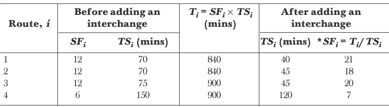
x1+ x2 + x3 + x4 + x5≤ 22 (ii) Table 3 shows the trip frequency per bus after adding the interchange. The daily operation hours is the product of the daily single trip per bus and the total time spent on a single trip.
Ti = SFi×TSi
where SFi is the daily single-trip frequency per bus and TSi is the total time spent on a single trip.
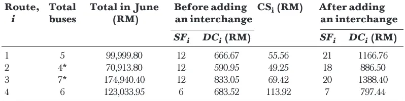
Table 4 displays the daily collection per bus before and after adding an interchange with the average daily collection per bus, DCi. The daily collection is calculated using the following formula;
i i
i i
TC DC
TJun TB
=
×
where TCi is the total number of days in June which is equals to 30 days and TBi is the total number of buses for route i. The collection per single trip per bus CSi is the proportion of daily collection over the value of the daily single trip frequency per bus, i.e.
Table 3 Trip frequency per bus after adding an interchange
Before adding an Ti = SFi× TSi After adding an
Route, i interchange (mins) interchange
SFi TSi (mins) TSi (mins) *SFi = Ti/TSi
1 12 70 840 40 21
2 12 70 840 45 18
3 12 75 900 45 20
4 6 150 900 120 7
i i
i
DC CS
SF
=
Notice that though from previous section it is mentioned that total number of buses to route 2 and route 3 are three and eight respectively, but in calculation for the average daily collection per bus DCi (column 5) in Table 4, the total number of buses for these two routes are taken as four and seven respectively. This is because the company’s original policy was to allocate four buses to route 2 while seven buses to route 3. However, the real situation shows that the passenger demand to route 3 is quite high compare to route 2. Due to the demand, one bus for route 2 is often transferred to route 3 but the bus fare collected still been recorded as the collection for route 2.
Constraint (iii) represents the minimum daily collection which should be achieved by each bus in order to cover the maintenance fees and labour cost. The company’s daily collection targeted for every bus is RM750. However, the record of daily collection in June 2003 shows that none of the buses hit the target in that month. We have changed the target to RM650 to obtain an optimal solution from the model developed. Thus, the original inequality becomes:
1166.76x1 + 886.50x2 + 1388.40x3 + 797.44x4≥ 650(x1+ x2 + x3 + x4) 516.76x1 + 236.50x2 + 738.40x3 + 147.44x4≥ 0
Table 4 Daily collection per bus before and after adding an interchange
Route, Total Total in June Before adding CSi (RM) After adding i buses (RM) an interchange an interchange
SFi DCi (RM) SFi DCi (RM)
1 5 99,999.80 12 666.67 55.56 21 1166.76
2 4* 70,913.80 12 590.95 49.25 18 886.50
3 7* 174,940.40 12 833.05 69.42 20 1388.40
4 6 123,033.95 6 683.52 113.92 7 797.44
Constraints (iv) of the model developed is given by the ratio of the total time for buses of route i to travel from terminal j to the terminus i then back to terminal j where
The idea of constraints (v) is almost the same as constraint (iv) and is given by:
min
ij i
TR x
h ≤
Minimum desired headway indicates that the minimum time range between two arrivals of the buses of the same route.
The mathematical programming model can be expressed as:
Max z = 1166.76x1 + 886.50x2 + 1388.40x3 + 797.44x4 (i)
Subject to x1 + x2 + x3 + x4 + x5≤ 22 (ii)
516.76x1 + 236.50x2 + 738.40x3 + 147.44x4≥ 0 (iii)
f1hmaxx1≥ 80
f2hmaxx2≥ 90
f3hmaxx3≥ 90 (iv)
f4hmaxx4≥ 240
hmaxx5≥ 56
hminx1≤ 80
hminx2≤ 90 (v)
hminx3≤ 90
hminx4≤ 240
4.0 COMPUTATIONAL RESULTS
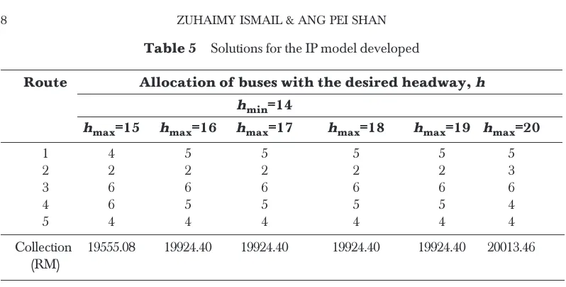
In searching for an optimal solution, different values of hmax and hmin are assigned and replaced in the model. If f1 = 2, f2 = f4 = 4 and f3 = 1 were fixed then this becomes a solution for route 1, 2, 3, 4 which is 28, 47, 19, and 50 minutes respectively. The results obtained using QM for window package is given in Table 5.
5.0 BUS RE-SCHEDULING
Due to the frequent overlapping between buses, it was necessary to reschedule the services which will minimize the frequency of buses departing from Larkin simultaneously. A series of rules and assumptions were developed based on some current and desired practices as follows:
(1) A maximum of two buses of different route can depart from Larkin at the same time. (2) Layover (idle time spent at terminal) for buses of route 1, 2 and 3 is 5 minutes
while a maximum of 10 minutes for buses of route 4. There must be layover for some recording work at Larkin Terminal and for bus crews to take a short break. Layover for route 4 is longer compare to other routes since its round-trip time is also much longer than others and we assume that the drivers need more time to rest. (3) Time interval between two departures at terminal Larkin is 0-15 minutes (20 minutes
can only be accepted during non-peak hour). Peak hours refer to 7:00 am-8:30 am and 5:00 pm-6:30 pm and the trip frequency should either be maintained or increased to satisfy the increasing demand.
(4) Table 6 shows the number of buses that start the daily work at terminal Larkin and the terminus respectively:
(5) The total round-trip time spent by every bus is estimated from the time study are carried out and the record of HISB.
(6) Every route must have at least one bus that arrives at Larkin Terminal between 7 am to 7.40 am and 8 am to 8.40 am (except Ayer Hitam - it is too early for a bus from Ayer Hitam to depart by 5.10 am in order to reach Larkin terminal before 7.40 am), assuming that office hour starts at either 8 am or 9 am.
(7) The last trip of the day for each bus ends when they reach Larkin or the terminus after 10.10 pm except for buses of route 4 which end after 9.30 pm as they take 2 hours 30 mins to end their one-way trip.
Table 5 Solutions for the IP model developed
Route Allocation of buses with the desired headway,h hmin=14
hmax=15 hmax=16 hmax=17 hmax=18 hmax=19 hmax=20
1 4 5 5 5 5 5
2 2 2 2 2 2 3
3 6 6 6 6 6 6
4 6 5 5 5 5 4
5 4 4 4 4 4 4
Collection 19555.08 19924.40 19924.40 19924.40 19924.40 20013.46 (RM)
Table 6 Number of buses that start daily operation at Larkin and the terminus
Route Number of buses start operation at: Total buses Larkin Terminus
1 - 5 5
2 - 3 3
3 4 4 8
(8) Buses are scheduled at an interval of 5 mins.
(9) The earliest departure time allowed is at 5.55 am. It should not be too early as not many passengers will be travelling that early in the morning.
Some assumptions are made to simplify the scheduling process: (1) All buses travel with almost the same and constant speed.
(2) Travel time of buses is always constant despite the time of the day.
For route i {i = 1, 2, 3, 4}, notations below are introduced:
Bi = Total number of buses to route i Li = Layover for buses to route i
T Ti = Total time spent for a round-trip journey of route i (Ti = RTi + Li)
hi = Headway for route i, i
i i T h
B
=
5.1 Headways Determination
Headway is the time between two bus arrivals of the same route. It is determined by dividing Ti by Bi in order to obtain a more constant headway throughout the day. Headways for each route are shown in Table 7.
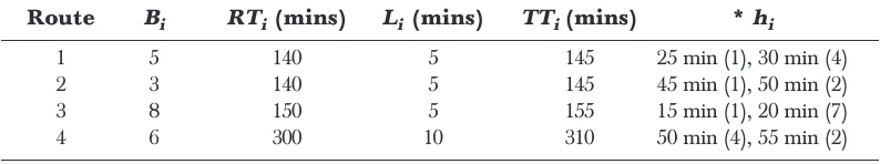
Table 7 Bus travel time and average headways for each route
Route Bi RTi (mins) Li (mins) TTi (mins) * hi
1 5 140 5 145 25 min (1), 30 min (4)
2 3 140 5 145 45 min (1), 50 min (2)
3 8 150 5 155 15 min (1), 20 min (7)
4 6 300 10 310 50 min (4), 55 min (2)
* Since buses are scheduled every 5 mins, the headways for the routes are not equally distributed. Numbers in the brackets indicate the number of buses with such interval.
6.0 RESULTS AND DISCUSSIONS
The first step in the scheduling process should be setting up of starting time for every route as describe in rule (6). For certain route, certain buses do not require to start from Larkin Terminal daily, this will ensure that there is at least one bus arriving at the main terminal between 7:00 am - 7:40 am and 8:00 am - 8:40 am. The earliest starting time was recorded at 5:55 am (this is rule (9)) except for route 4.
single bus of the route by referring to rules (2) and (5) and also headways determined in Table 7. After that, we try to arrange the schedule for the remaining route by considering rules (1), (2), (3) and (5) and the schedule of the arbitrary route as well. We try not to change the schedule of the arbitrary route to simplify the process. Anyhow, the interval between two buses is adjustable based on the headways determined in Table 6.
In this case, route 4 is the last one to be scheduled as it is more independent since its round-trip time is twice the distance than the others and the overlapping part of the journey is small. Moreover, it is more flexible as its layover can be either 5 minutes or 10 minutes in order not to violate rule (1) and also to maintain rule (3).
Several schedules were constructed based on the steps above. Schedule which cannot satisfy either of the rules will be eliminated. The schedule with the least 20 minutes time interval between two departures is selected as the solution. Results from the proposed model shows that the maximum collection that can be obtained is RM20013.46 with the minimum headway, hmin of each route is 14 minutes, and the greatest common factor of the desired headway for every route, hmax is 20 minutes. We realized that the solution is not that desirable since the headway for current practice is 28 minutes, 47 minutes, 19 minutes and 50 minutes for route 1, 2, 3 and 4 respectively. The headway for route i, hi is given by:
i i
i RT h
B
=
where RTi is the round trip time for route i (i = 1, 2, 3, 4, 5) and Bi be the total number of buses to route i (i = 1, 2, 3, 4, 5).
The solution shows a great improvement in the time interval between two bus arrivals for route 1 and route 2 but also a big decrement in time interval between two bus arrivals for route 4.
The maximum collection that was obtained from the calculation costs a total of RM19, 924.40. It shows that there exist several values of hmax which will produce this optimal solution. These solutions have the same minimum headway, hmin of 14 minutes. Notice that these optimal solutions actually carry the same result as in the allocation of buses to each route. It can be seen that the values of hi is between 14 and 48. Thus, hi
The value of hi should be adjusted to (i, hi) = (1, 16), (2, 48), (3, 16), (4, 48), (5, 16) with hmax = 16 in order to reduce the number of buses needed in route 5. The percentage of increment in collection can be calculated as follows:
100
19 924 40 15 629 60 100 15 629 60
27 48 AI CP
PI %
CP
, . , .
%
, .
. % −
= ×
−
= ×
=
where PI is the percentage of increment; AI is the total daily collection if added an interchange and CP is the total daily collection for current practice with the total daily collection of current practice
Total collection in June for all 4 routes Total days in June
99 999 80 70 913 80 174 940 40 123 033 95 90
RM15 629 60
, . , . , . , .
, .
=
+ + +
= =
Bus rescheduling may be one of the ways to reduce cost but unfortunately it is time consuming. It is worst with problem with large fleet size. Many real world situations do not take into account factors such as inelastic passenger demand where trip frequency might need to be increased during peak hours (this will then contradict with the rule of constant headway unless extra buses are provided). Issues such as traffic jam during peak hours that might cause delays are also not being considered in this case. However, the proposed schedule is able to handle the problem of unhealthy competition within the company’s own buses if the buses stick to the schedule (for the
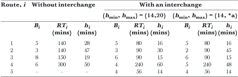
Table 8 Headway of each route before and after introducing an interchange
Route, i Without interchange With an interchange
(hmin, hmax) = (14,20) (hmin, hmax) = (14, *a)
Bi RTi hi Bi RTi hi Bi RTi hi
(mins) (mins) (mins) (mins) (mins)(mins)
1 5 140 28 5 80 16 5 80 16
2 3 140 47 3 90 30 2 90 45
3 8 150 19 6 90 15 6 90 15
4 6 300 50 4 240 60 5 240 48
5 - - - 4 56 14 4 56 14
departure time from Larkin Terminal) and not trying to overtake their company buses to race for passengers while on the road.
The Excel program designed can overcome this problem in a more systematic way [4]. This program only satisfies the current situation in HISB Company where there are only six kinds of routes and a maximum of fifty tasks available. Besides, the drivers will only be given a same task for the whole week and the duty schedule is only rearranged once a week. However, these rules and limitations can easily be modified according to the situation. In fact, in real situation, the manpower available should be more than the total number of tasks offered since every driver will have at least an off day each week and a person to replace when any drivers take medical or other leaves. In this case, we propose the company to hire several part timers where their task is to fill in the blank duties. Their duties will not be scheduled using the program developed and thus they might not have a same duty everyday.
In our study, we took the total number of buses operating daily for all routes as the total number of tasks offered as well. We proposed the total number of tasks per shift,
NT by:
TR
NT L
WD
= ×
where TR is the total number of buses operating daily for all routes, L is the length (in days) of a schedule and WD is the number of working days in the schedule.
For instance, currently there are a total of 34 buses operating daily and the bus-crew timetable is arranged once a week. Assume that the drivers work 6 days a week. Hence the total number of tasks is given by:
34 7 6 39 67 39 or 40 NT
.
= ×
= ≈
The problem is that we cannot easily get an integer value for number of tasks of each route using the same formula above. Select the largest integer ≤NT if the company wants to reduce labour cost but then the working days for some bus crews will be more than the WD set earlier; else choose the smallest integer ≥NT so that there will be someone standing by in case there are bus crews taking leaves and no drivers want to work overtime. Therefore, the program has to be modified and some drivers will be assigned to mixed duties, i.e. driving two or more routes in a week. Anyway, this process will be much more complicated.
place at the interchange and also the labour cost of staffing at the interchange. The company should compare the increment in collection after introducing an interchange with the costs involved then determined whether the idea is worth implementing. The increment of collection per month, I is estimated as follows:
( )
( )
Total days in June
19 924 40 15 629 60 30
RM128 844 00
I AI CP
, . , .
, .
= − ×
= − ×
=
The labour cost should not be an issue since only a few staffs are needed for the bus operations at the interchange. The cost of applying and adding the interchange might cost a lot to the company but it may gain back the investment quickly if the estimated collection is maintained or improved in the real situation [5].
The company might have some concern about the customers’ response since shifting to another bus is somehow troublesome. Commuters might rather take the buses from other companies to avoid this problem [6]. In order to attract the commuters, the company can take some steps such as offering a cheaper bus fare to them. For example, if the company gives a 5 percent discount for the bus fare, there will still be an increment in the collection with new percentage of increment, NI in collection obtained by using the formula of PI (1) but times AI with (100%-discount rate), i.e.
( )
19 924 40 100 5 15 629 60
100 15 629 60
21 10
, . % , .
NI %
, . . %
× − −
= ×
=
The value of I is estimated as follows:
(
)
( )
100 discount rate Total days in June
19 924 40 95 15 629 60 30
RM98957 40
I AI % CP
, . % , .
.
= × − − ×
= × − ×
=
This is a win-win situation where both the company and passengers will gain from this arrangement.
the scheduling process since doing this job manually is time consuming especially when trying to construct a schedule which seems fair to all drivers.
ACKNOWLEDGEMENTS
We wish to thank the Department of Mathematics, Universiti Teknologi Malaysia and HISB for their full collaboration in assisting the team in this project.
REFERENCE
[1] Belletti, R., A. Davini, P. Carraresi, and G. Gallo. 1985. BDROP: A Package for the Bus Driver’s Rostering Problem, North-Holland Publishing Company.
[2] Hagberg, B. 1985. An Assignment Approach to the Rostering Problem: An Application to Taxi Vehicle. North-Holland Publishing Company.
[3] Bramel, J., and D. Simchi-Levi. 1996. Probabilistic Analysis and Practical Algorithm for the VRP aith Time Windows. Operations Research. 44: 501-509.
[4] Ceder, A. 2000. Efficient Timetabling and Vehicle Scheduling for Public Transport. Paper presented at the 8th International Conference on Computer-Aided Scheduling of Public Transport (CASPT).
[5] Jean-Francois, and G. Laporte. 2002. Tabu Search Heuristics for the Vehicle Routing Problem. Canada Research Chair in Distribution Management and GERAD.
[6] Dirk, L. V. O., and W. Zhi. 1995. Trip Frequency Scheduling for Bus Route Management in Bangkok.