Accelerating the Simulation of Chemically Reacting Turbulent Flows via Machine Learning Techniques.

ABSTRACT

OWOYELE, OPEOLUWA OLAWALE. Accelerating the Simulation of Chemically Reacting Turbulent Flows via Machine Learning Techniques. (Under the direction of Dr. Tarek Echekki).

Accelerating the Simulation of Chemically Reacting Turbulent Flows via Machine Learning Techniques

by

Opeoluwa Owoyele

A dissertation submitted to the Graduate Faculty of North Carolina State University

in partial fulfillment of the requirements for the degree of

Doctor of Philosophy

Mechanical Engineering

Raleigh, North Carolina 2018

APPROVED BY:

_______________________________ _______________________________

Dr. Tarek Echekki Dr. Tiegang Fang Committee Chair

_______________________________ _______________________________

ii DEDICATION

To my parents:

iii BIOGRAPHY

iv ACKNOWLEDGMENTS

Firstly, I would like to thank my advisor, Professor Tarek Echekki, for his guidance and mentorship during my PhD. I walked into his office about 3 and half years ago seeking to be his PhD student, and in spite of not having any experience in combustion modeling, he was willing to have me as his student. Today, virtually all I know regarding combustion modeling has been learned by virtue of my research under him. His patience and consideration, physical insight and knowledge of the field has made working with him a pleasant experience. I would also like to thank the members of the committee, Dr. Alexei Saveliev, Dr. Phillip Westmoreland and Dr. Tiegang Fang for their service and for bringing different dimensions of constructive criticisms to my work. My appreciation also goes to those I collaborated with during my PhD. Specifically, I would like to thank Dr. Sibendu Som, Dr. Prithwish Kundu and Dr. Muhsin Ameen. In addition, my appreciation goes to Dr. Jacqueline Chen and Dr. Aditya Konduri of Sandia National Laboratory.

I would also like to appreciate various colleagues that I worked with during this time. My former colleagues at the lab – Dr. Hessam Mirgolbabaei, Dr. Andreas Hoffie, Dr. Sami Ben Rejeb and Mr. TJ Wignall – were helpful when I had just joined and was trying to get my feet wet. Furthermore, being labmates with Mr. Sultan Alqahtani and Mr. Rishikesh Ranade has been amazing. I'll like to thank them for the many fruitful discussions we've had both in and out of the lab, and I wish them the best in their quest to obtain their doctorate degrees as well.

v whose selfless sacrifices and love for me continue to inspire me to this day. I cannot overstate how important the lessons I have learned from the words and examples of my parents have been. I could never have made it this far without them. I'll also like to appreciate my siblings, especially AK, for supporting me throughout the years. My church family here in Raleigh have been my family away from home. While I cannot list everyone, specifically, I would like to thank Sean Steadley for being a wonderful roommate, friend and brother. Getting to know you is one of the reasons why I am glad that I moved to Raleigh, and why I am sad that I get to move away. I would also like to appreciate Lisa Steadley, for her energetic labor of love and for being a source of immense blessing, over and over again to my wife and me.

To my wife, Idunumi – the love of my life and mother of my newborn: thank you for all the days you were patient when I had to work almost all the time on research, and for understanding that this is not about me alone, but about our family. Thank you for your prayers, delicious meals and encouragement. A wife like you is truly hard to find, and I hope I spend the rest of our days together showing you how much I love you.

vi TABLE OF CONTENTS

LIST OF TABLES ... viii

LIST OF FIGURES ... ix

Introduction... 1

1.1 Combustion Modelling ... 2

1.2.1 Direct Numerical Simulation ... 2

1.2.2 Large Eddy Simulation and Reynolds Averaged Numerical Simulation ... 3

1.2 Machine Learning ... 7

1.2.1 Unsupervised Machine Learning ... 8

1.2.2 Supervised Machine Learning ... 9

1.2.3 Machine Learning in Combustion ... 10

1.3 Objectives ... 13

1.4 Outline... 15

Model formulation and governing equations ... 18

2.1 Principal Components Analysis ... 18

2.1.1 Dimensionality reduction using PCA ... 18

2.1.2 Mathematical Construction of Principal Components ... 20

2.2 Artificial Neural Networks ... 21

2.2.1 ANN structure ... 22

2.2.2 ANN Algorithm ... 24

2.3 Governing Equations ... 25

2.3.1 Species’ transport governing equations ... 25

2.3.2 Governing equations for Principal Components ... 27

2.3.3 The Flamelet Model ... 28

2.3.3 Turbulence Models ... 29

Transport of Principal Components in a Vortical Flow Field ... 32

3.1 A priori analysis ... 33

3.2 Procedure for a posteriori validation ... 36

3.3 PCA-ANN using unity Lewis number diffusion formulation... 39

3.3.1 Numerical Implementation and Problem setup... 39

vii

3.4 PCA-ANN using mixture-averaged diffusion formulation... 68

3.4.1 Numerical Implementation and Problem setup... 68

3.4.2 Results ... 75

3.5 n-Heptane Bunsen Case: an a priori analysis ... 108

3.6 Time Savings and Discussion ... 112

3.5.1 Discussion of Results ... 112

3.5.2 Time Savings ... 115

Application of Machine Learning to the Tabulated Flamelet Model ... 118

4.1 Methodology ... 121

4.2 Computational Setup ... 124

4.2.1 4D Spray A Simulations ... 124

4.2.2 5D Compression ignition Engine Simulations ... 129

4.3 Results and Discussion ... 132

4.3.1 ECN Spray A case ... 132

4.3.2 Compression Ignition Engine case... 172

4.4 Memory Requirements... 178

Conclusion and Future Work ... 181

5.1 Summary ... 181

5.2 Future Work ... 184

REFERENCES ... 187

APPENDICES ... 200

Appendix A Transport Properties ... 201

A.1 Simplified Diffusion Coefficients ... 201

viii LIST OF TABLES

Table 3.1 Comparison of the two PCA-ANN cases considered. ... 38

Table 3.2

∆

t

Table 3.3 for the principal components. ... 63

Table 3.4 Summary of computational requirements. ... 70

Table 3.5 ε at t = 0.3ms. Variables in boldface correspond to the selected subset for PCA ... 95

Table 3.6

∆

t

Table 3.7 for the principal components. ... 102

Table 4.1 ECN Spray A experimental conditions. ... 125

Table 4.2 Boundary conditions for Spray A ... 126

Table 4.3 Computational set up for LES and RANS simulations ... 129

Table 4.4 Optical Engine Setup ... 131

Table A.1 Collision integral coefficientsa_i(1) anda_i(2)[29,87]. ... 203 1%

t

∆

1% t

ix LIST OF FIGURES

Figure 1.1 Classes of Machine Learning algorithms. ... 8 Figure 2.1 Illustration of the transformation of a sample variable system to a

principal component space. ... 20 Figure 2.2 Typical structure of an artificial neural network. ... 23 Figure 3.1 A priori steps involved in the construction of PCs and ANN training. ... 34 Figure 3.2 Comparison of the transport of thermochemical scalars and the

PC-transport approach. ... 37 Figure 3.3 Scree plot for the correlation matrix based on all 17 (filled triangle)

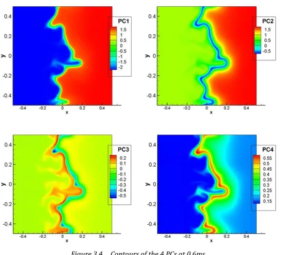
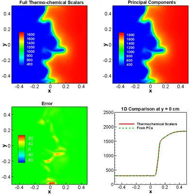
and 7 (filled circles) major variables. ... 42 Figure 3.4 Contours of the 4 PCs at 0.6ms. ... 45 Figure 3.5 Contours of thermochemical scalars (top left) and PCs (top right) DNS

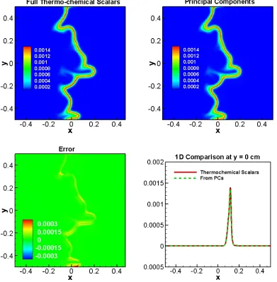
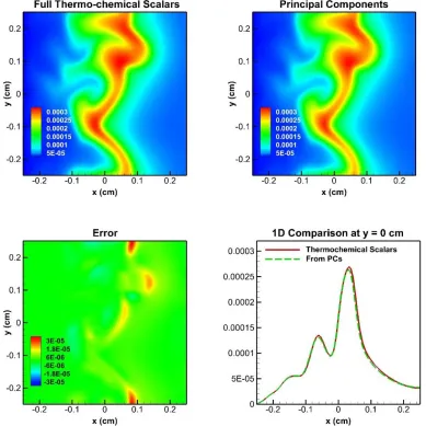
predictions of Temperature at 0.6ms and the errors (bottom left) and a 1D cut of profile at y = 0cm. ... 47 Figure 3.6 Contours of thermochemical scalars (top left) and PCs (top right) DNS

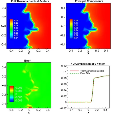
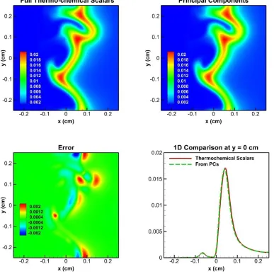
predictions of H2O at 0.6ms and the errors (bottom left) and a 1D cut of profile at y = 0cm. ... 48 Figure 3.7 Contours of thermochemical scalars (top left) and PCs (top right) DNS

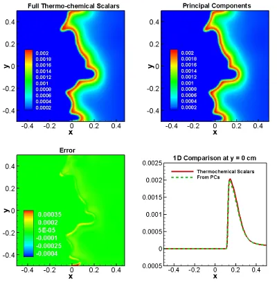
predictions of CO2 at 0.6ms and the errors (bottom left) and a 1D cut of profile at y = 0cm. ... 49 Figure 3.8 Contours of thermochemical scalars (top left) and PCs (top right) DNS

predictions of H2 at 0.6ms and the errors (bottom left) and a 1D cut of profile at y = 0cm. ... 51 Figure 3.9 Contours of thermochemical scalars (top left) and PCs (top right) DNS

predictions of CO at 0.6ms and the errors (bottom left) and a 1D cut of profile at y = 0cm. ... 52 Figure 3.10 Contours of thermochemical scalars (top left) and PCs (top right) DNS

predictions of O at 0.6ms and the errors (bottom left) and a 1D cut of profile at y = 0cm. ... 54 Figure 3.11 Contours of thermochemical scalars (top left) and PCs (top right) DNS

predictions of OH at 0.6ms and the errors (bottom left) and a 1D cut of profile at y = 0cm. ... 55 Figure 3.12 Contours of thermochemical scalars (top left) and PCs (top right) DNS

predictions of CH2O at 0.6ms and the errors (bottom left) and a 1D cut of profile at y = 0cm. ... 56 Figure 3.13 Contours of thermochemical scalars (top left) and PCs (top right) DNS

predictions of CH3 at 0.6ms and the errors (bottom left) and a 1D cut of profile at y = 0cm. ... 58 Figure 3.14 Contours of thermochemical scalars (top left) and PCs (top right) DNS

x Figure 3.15 Contours of thermochemical scalars (top left) and PCs (top right) DNS

predictions of CH3O at 0.6ms and the errors (bottom left) and a 1D cut of profile at y = 0cm. ... 60 Figure 3.16

∆

t

0.3ms. ... 71 Figure 3.19 Scree plot for the correlation matrix based on all 31 (filled squares)

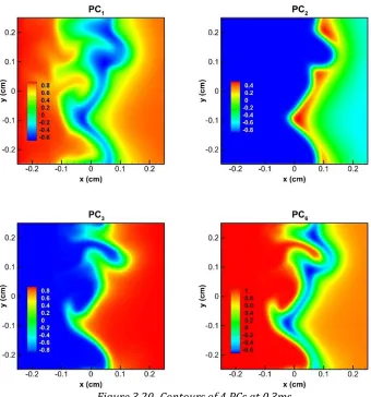
and 8 (filled diamonds) selected variables. ... 74 Figure 3.20 Contours of 4 PCs at 0.3ms. ... 76 Figure 3.21 Contours of thermochemical scalars (top left) and PCs (top right) DNS

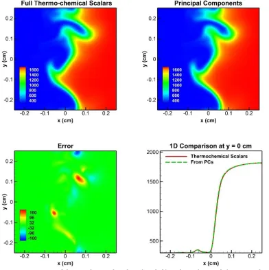
predictions of Temperature at 0.3ms and the errors (bottom left) and a 1D cut of profile at y = 0cm. ... 79 Figure 3.22 Contours of thermochemical scalars (top left) and PCs (top right) DNS

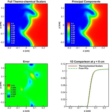
predictions of CO2 mass fraction at 0.3ms and the errors (bottom left) and a 1D cut of profile at y = 0cm. ... 80 Figure 3.23 Contours of thermochemical scalars (top left) and PCs (top right) DNS

predictions of H2 mass fraction at 0.3ms and the errors (bottom left) and a 1D cut of profile at y = 0cm. ... 81 Figure 3.24 Contours of thermochemical scalars (top left) and PCs (top right) DNS

predictions of CO mass fraction at 0.3ms and the errors (bottom left) and a 1D cut of profile at y = 0cm. ... 82 Figure 3.25 Contours of thermochemical scalars (top left) and PCs (top right) DNS

predictions of O mass fraction at 0.3ms and the errors (bottom left) and a 1D cut of profile at y = 0cm. ... 83 Figure 3.26 Contours of thermochemical scalars (top left) and PCs (top right) DNS

predictions of H mass fraction at 0.3 ms and the errors (bottom left) and a 1D cut of profile at y = 0cm. ... 84 Figure 3.27 Contours of thermochemical scalars (top left) and PCs (top right) DNS

predictions of HO2 mass fraction at 0.3 ms and the errors (bottom left) and a 1D cut of profile at y = 0cm. ... 87 Figure 3.28 Contours of thermochemical scalars (top left) and PCs (top right) DNS

predictions of CH2 mass fraction at 0.3 ms and the errors (bottom left) and a 1D cut of profile at y = 0cm. ... 88 Figure 3.29 Contours of thermochemical scalars (top left) and PCs (top right) DNS

predictions of CH2O mass fraction at 0.3ms and the errors (bottom left) and a 1D cut of profile at y = 0cm. ... 89 Figure 3.30 Contours of thermochemical scalars (top left) and PCs (top right) DNS

predictions of CH3OH mass fraction at 0.3ms and the errors (bottom left) and a 1D cut of profile at y = 0cm. ... 90 Figure 3.31 Contours of thermochemical scalars (top left) and PCs (top right) DNS

xi Figure 3.32 Contours of thermochemical scalars (top left) and PCs (top right) DNS

predictions of CH2CO mass fraction at 0.3ms and the errors (bottom

left) and a 1D cut of profile at y = 0cm. ... 92

Figure 3.33 O mass fraction at different times during flame evolution for 1D tabulation. Regions of localized departure from true physics are circled. ... 96

Figure 3.34 CH2O mass fraction at different times during flame evolution for 1D tabulation. Regions of localized departure from true physics are circled. ... 97

Figure 3.35 Spatial resolution requirements for selected species and the PCs. ... 103

Figure 3.36 Slices of the mass fraction of O with an isocontour (top right) at 0.00025. ... 105

Figure 3.37 Slices of the mass fraction of CH2O with an isocontour (top right) at 0.0002 ... 105

Figure 3.38 Slices of the temperature with an isocontour (top right) at 1000K. ... 106

Figure 3.39 Slices of HO2 mass fraction with an isocontour (top right) at approximately one-fourth of its maximum value. ... 107

Figure 3.40 Domain boundary conditions for Bunsen burner with temperature marker at 1450K. ... 108

Figure 3.41 Scree plot for the Bunsen burner case. ... 109

Figure 3.42 Temperature (left) and CO mass fraction (right) profiles at t=0.4ms. ... 110

Figure 3.43 Profiles of PC1 (left) and PC8 (right) at t=0.4ms. ... 111

Figure 3.44 Savings in the number of transported variables for different mechanism sizes. ... 113

Figure 4.1 Spray A computational domain. ... 126

Figure 4.2 Training errors for the 4D table vs. the number of layers in the ANN. ... 134

Figure 4.3 Regression plot of selected species for the case where each specie has a unique ANN. ... 135

Figure 4.4 Regression plot for the case where a single ANN is used to predict the mass fractions of all the species ... 137

Figure 4.5 Time taken to retrieve the mass fractions of all 24 species as a function of the number of groups ... 138

Figure 4.6 Flowchart demonstrating the algorithm used for grouping the species based on the matric of correlation coefficients. ... 140

Figure 4.7 Matrix of correlation coefficients for all the species. ... 142

Figure 4.8 Correlation coefficients for group 1 ... 143

Figure 4.9 Correlation coefficients for group 2 ... 143

Figure 4.10 Correlation coefficients for group 3 ... 144

Figure 4.11 Correlation coefficients for group 4 ... 144

Figure 4.12 Correlation coefficients for group 5 ... 145

Figure 4.13 Correlation coefficients for group 6. ... 145

xii Figure 4.15 Mass fraction predictions of the main reactants and products for

TFM-ANN 1, TFM-ANN 2, and the flamelet table at a low scalar

dissipation rate. ... 148 Figure 4.16 Mass fraction predictions of the radicals and other main intermediates

for TFM-ANN 1, TFM-ANN 2, and the flamelet table at a low scalar

dissipation rate ... 149 Figure 4.17 Mass fraction predictions of other intermediates and nitrogen for

TFM-ANN 1, TFM-ANN 2, and the flamelet table at a low scalar

dissipation rate. ... 150 Figure 4.18 Mass fraction predictions the main products and reactants for

TFM-ANN 1, TFM-ANN 2, and the flamelet table at a scalar

dissipation rate of 10s-1. ... 152 Figure 4.19 Mass fraction predictions of the radicals and other main intermediates

for TFM-ANN 1, TFM-ANN 2, and the flamelet table at a scalar

dissipation rate of 10s-1. ... 153 Figure 4.20 Mass fraction predictions of other intermediates and nitrogen for

TFM-ANN 1, TFM-ANN 2, and the flamelet table at a scalar

dissipation rate of 10s-1. ... 154 Figure 4.21 Mass fraction predictions of the main products and reactants for

TFM-ANN 1, TFM-ANN 2, and the flamelet table at a scalar

dissipation rate of 100s-1. ... 155 Figure 4.22 Mass fraction predictions of the radicals and other main intermediates

for TFM-ANN 1, TFM-ANN 2, and the flamelet table at a scalar

dissipation rate of 100s-1. ... 156 Figure 4.23 Mass fraction predictions of other intermediates and nitrogen for

TFM-ANN 1, TFM-ANN 2, and the flamelet table at a scalar

dissipation rate of 100s-1. ... 157 Figure 4.24 Ignition delay as a function of ambient temperature conditions with

LES and RANS models using ANNs. ... 159 Figure 4.25 Flame liftoff (right) as a function of ambient temperature conditions

with LES and RANS models using ANNs. ... 159 Figure 4.26 The temporal evolution of the cool flame region i.e. CH2O mass

fraction contours predicted by theTFM- ANN LES model (center) are compared against the TFM model (right) and CH2O PLIF data [82] (left) from a single shot. ... 162 Figure 4.27 The temporal evolution of the OH mass fraction contours predicted by

theTFM- ANN model (center) are compared against the TFM model (right) and OH PLIF data [83] (left). ... 163 Figure 4.28 LES (left column) and RANS (right column) contour plots of

temperature on the middle y-plane at various ambient temperatures. ... 165 Figure 4.29 LES (left column) and RANS (right column) contour plots of OH

xiii Figure 4.30 LES (left column) and RANS (right column) contour plots of CH2O

mass fraction on the middle y-plane at various ambient temperatures. ... 167 Figure 4.31 LES (left column) and RANS (right column) contour plots of CO2

mass fraction on the middle y-plane at various ambient temperatures. ... 168 Figure 4.32 LES (left column) and RANS (right column) contour plots of CO mass

fraction on the middle y-plane at various ambient temperatures. ... 169 Figure 4.33 LES (left column) and RANS (right column) contour plots of H2 mass

fraction on the middle y-plane at various ambient temperatures. ... 170 Figure 4.34 Pressure trace from the motored engine case compared with the

experimental values [77]. ... 172 Figure 4.35 Pressure trace obtained from the RANS and LES simulations compared

against experimental values [77]. ... 174 Figure 4.36 Heat relase rates obtained from the RANS and LES simulations

compared against experimental values [77]. ... 174 Figure 4.37 Flame liftoff from experiments [77] compared against the RANS and

LES with the TFM-ANN model. ... 175 Figure 4.38 Contour plots of temperature (left column) and OH mass fraction (right

column) at varying crank angle degrees along the plane of the spray. ... 176 Figure 4.39 Contour plots of (a) scalar dissipation rate, (b) CH2O mass fractions,

(c) OH mass fractions and (d) temperature at 5 crank angle degrees after top dead center along the plane of the spray. ... 177 Figure 4.40 Memory (RAM) consumed per processor as a function of the

simulation time for the Spray A LES case with TFM and TFM-ANN

approach and a 4D manifold. ... 179 Figure 4.41 Memory (RAM) consumed per processor as a function of the

1

Introduction

The complexity of turbulent combustion is highlighted by the fact that it combines two

very complex and challenging aspects of science: turbulence and combustion. For

thousands of years, combustion has been used as a form of cooking and heating.

Relatively recently, however, combustion has found application in many more areas of

human existence, including the internal combustion engine, propulsion, industry and

power generation. Even more recently, the invention of the computer and the subsequent

burgeoning of computing power has led to advances in the implementation of computer

simulations of the behavior of fluids, referred to as computational fluid dynamics (CFD).

The non-linear equations which describe the motion of fluids, referred to as the

Navier-Stokes equations, have been named as one of the most important problems in

mathematics by the Clay Mathematics Institute [1]. Till date, these equations remain

without an analytical solution, and are thus solved numerically by the use of CFD tools.

In turbulent combustion, in addition to the complexity introduced by an unsteady

turbulent velocity field, the fluid goes through rapid chemical changes which alter the

composition and property of the fluid. There is also a spontaneous release of energy,

resulting in rapid temperature rise as the fuel is burned. These result in a two-way

2

extreme turbulence, while changes in properties such as viscosity can damp turbulent

eddies.

1.1 Combustion Modelling

The computational tools used perform computer simulations of turbulent combustion

can be divided into three parts, viz,

1. Direct numerical simulation

2. Reynolds-averaged Navier-Stokes simulation (RANS)

3. Large eddy simulation (LES)

1.2.1 Direct Numerical Simulation

Given the availability of accurate chemistry models, direct numerical simulation (DNS)

provides an accurate benchmark against which other methods that model

turbulence-chemistry interactions (TCI) can be measured, because all time and spatial length scales

are resolved. However, currently, DNS remains largely confined to theoretical problems

within the four walls of the laboratory for two reasons.

The first problem is the presence of a large range of scales in space and time. The scales

in time could range from 10-10_{s to a few seconds [2] (the timescale relating to NOx}

production), and the full range of these scales need to be solved – or modelled in the case

3

processes) to the size of the combustor (for the larger turbulence structures). These two

problems – multiscale phenomena in space and time which means we need to solve a stiff

system within a fine grid – jointly require large number of points where the

thermochemical (consisting of temperature and species’ mass factions) and velocity

vector need to be solved in order to obtain a stable and accurate solution.

The second problem is the presence of large number of species. Hydrogen mechanisms

used in combustion simulations, based on a relatively simple fuel, can have over ten

species and tens of reactions. Thus, in addition to the aforementioned challenge – a high

number of solutions of the thermochemical vector in space and time – a new challenge

arises: a large thermochemical vector. However, hydrogen is still not a practical fuel for

commercial applications due to the absence of an economically viable means for its

production. Practical fuels are usually a blend of hydrocarbons, for which detailed and

skeletal fuels mechanisms can contain between tens to hundreds of species and hundreds

to several thousands of reactions. Furthermore, in addition to the burden of transporting

a large number of species, evaluating the source term is computationally expensive as it

requires the evaluation of a large number of elementary reaction rates for each specie.

1.2.2 Large Eddy Simulation and Reynolds Averaged Numerical

Simulation

For RANS, as opposed to DNS where all the scales are resolved, only an ensemble average

4

in DNS. However, turbulence is inherently chaotic and RANS has the disadvantage of

presenting this chaotic phenomena as a well-behaved and smooth one. Also, commonly

observed behavior such as cycle-to-cycle variation in internal combustion engines and

highly local effects cannot be captured using RANS simulations. LES, on the other hand,

is able to capture these effects. Since in non-reacting turbulence, the bulk of the energy

of the flow comes from the larger scales before being passed to the smaller length scales

where they are dissipated by heat, in LES only the larger scales are solved for, while the

smaller scales are modelled. In terms of computational resources, LES typically requires

computing power which lies between RANS and DNS, depending on the size of the filter

used, a fine filter being closer to DNS and a coarse filter closer to RANS.

In RANS and LES, because averaged or filtered quantities are solved for, there are always

unclosed terms that need to be modeled. For turbulent combustion, many models have

been proposed to predict the averaged source term. Most of the closure models can be

classified as either flamelet-like models or pdf-like models.

1.2.2.1 PDF-Like Models

In PDF-like models, unclosed terms are modelled by the use of a joint probability density

function of fluid properties and species mass fractions. In most applications, as opposed

to assuming that the PDF has a predefined shape as in [3], the PDFs are determined by

the use of evolution equations. The idea of using PDFs to describe the turbulent flows

was introduced with the work of Lundgren [4], where he developed equations to describe

5

[5] extended this work to reacting flows in a paper published in 1974, where they derived

single and double point differential equations for the probability density function for a

two-reactant system undergoing a one-step chemical reaction. However, for practical

combustion systems with several species, finite-difference solutions to the PDF

equations are impractical due to the large dimensionality of these equations. In this case,

the computational cost rises exponentially with the number of independent variables.

Thus, Monte Carlo methods, developed by Pope [6], are typically used. In this case, the

computational cost rises only linearly with the number of independent variables. Also,

while the original formulations of the PDF equations were in Eulerian form, today

Lagrangian forms of the equations are typically used [7]. This typically involves the

introduction of notional particles, which are modelled after the Brownian motion of

particles, into the domain. For LES problems, a filtered density function is introduced.

PDF models have a number of advantages. They are computationally tractable, and are

very accurate, when compared to other RANS and LES combustion models. Additionally,

they are fairly generic and can be applied to a wide range of problems. Many other

combustion models are problem- or regime-specific. However, PDF models do not

address the “many species” problem and, in addition, involves the additional cost of

solving for the PDF. Although the prohibitive cost is highly mitigated by the use of Monte

Carlo methods, it is still computationally prohibitive and the error scales only with the

6 1.2.2.2 Flamelet-Like Models

When the time scales for chemical reactions are small compared to the convection and

diffusion time scales, we can reasonably assume that reaction takes place in thin reaction

zones that are relatively undistorted by the turbulent flow field [8]. Under this

assumption, it is further assumed that a flame is made up of an ensemble of these thin

reaction layers, embedded in the turbulent flow, referred to as flamelets. The flamelet

model is based on the “conserved scalar” approach where it is assumed that the entire

thermochemical state – consisting of temperature, density and mass fractions – can be

determined by the use of a conserved scalar. Peters (1984) extended this conserved

scalar approach to include non-equilibrium effects [9,10]. He showed that transforming

the coordinates to mixture fraction space leads to quasi-steady scalar profiles in mixture

faction space. Typically, these equation can be solved numerically in a CFD solver or a

representative problem can be run a priori, typically a counter-diffusion flame

configuration and the results stored in a table. The flamelet model has a number of

advantages. First, while it is evident that they may not be suitable for all kinds of flows,

the dimensionality of the manifold is reduced to about 3 or 4, thereby reducing the

number of independent variables to be solved. The problem is very simple compared to

some other models – the complex multidimensional chemical manifold is replaced by a

very simple lower dimensional manifold. The very small time and spatial scales in the

thermochemical space are eliminated – these, and the aforementioned advantages makes

7

typically involves the storage of large, multidimensional tables. In order to speed up the

simulation, the integration of the chemical space as a function of mixture fraction and

other independent variables can be performed a priori and stored in tables. This table is

stored in memory at the beginning of a CFD simulation and interpolation is performed

whenever species mass fractions are required as a function of independent variables.

This has an obvious drawback. Typically, large chunks of computer memory must be

dedicated to store these tables. Moreover, it means that this method is largely restricted

to low-dimensional manifolds, as the size of the tables we need to store will rise sharply

with dimensionality.

1.2 Machine Learning

Through the use of machine learning techniques, we can use computer algorithms to find

patterns and functional relationships without explicit programming. Machine learning

can be supervised, when the output of the code is foreknown, or unsupervised, when we

rely on the computer to identify trends and data patterns. Supervised machine learning

can be used for regression or classification problems, depending on the kind of data we

have, and examples include artificial neural networks, support vector machines, gaussian

regression, and random forests. Examples of unsupervised machine learning include

principal components analysis and k-means clustering. Figure 1.1 shows a summary of

8

Figure 1.1 Classes of Machine Learning algorithms.

1.2.1 Unsupervised Machine Learning

Unsupervised machine learning refers to an area of machine learning which relies on

algorithms to find hidden patterns in data without specifying such information

beforehand. This is used for unlabeled data, when it is desired to learn more about poorly

understood data, and we rely on the computer to unearth such underlying structures. As

opposed to supervised machine learning where we specify output values or classes to be

assimilated by the computer program, here the learning algorithm is simply fed a

data-set and it identifies clusters or patterns. Generally, unsupervised machine learning

techniques can be used for the following:

1. Clustering: in some cases, we need to classify data into naturally occurring groups,

where those groups are not explicitly known beforehand. For example, an online

store may wish to cluster customers according to their spending patterns in order

to give more relevant product suggestions to customers. In many data-based

9

are very different. In clustering, the aim is to identify data that are similar to one

another and place them in the same group, while keeping dissimilar data in

different groups. As may be already evident, such a procedure is subjective.

Hence, some clustering analyses are described as “hard” and others as “soft,” the

former referring to situations where the boundaries between clusters are sharp,

and the latter referring to a system where we only describe the probability of a

certain point belonging to a given cluster. Examples of clustering include k-means

and hierarchical clustering.

2. Dimensionality reduction: many problems in science and engineering are defined

by a variable space, known a features. Also, in many cases, the number of variables

defining the feature space can be high. In reacting flows, for instance, the

composition space can be defined by as many as hundreds or thousands of

chemical species. Sometimes, these variables are not completely independent but

have some correlation to one another. Unsupervised machine learning can be

used to identify lower-dimensional manifolds, such that the size of the manifold is

reduced while preserving the relevant information in the dataset. Examples of

dimensionality reduction techniques include principal components analysis and

auto-encoders.

1.2.2 Supervised Machine Learning

Supervised machine learning is a class of machine learning methods where the outputs

10

experience,” thus being able to predict unseen data with reasonable certainty after being

trained on seen data. The learning process starts with a large error, and the program tries

to progressively adjust the parameters, so that the output of the program approaches the

desired output. Supervised machine learning can broadly divided into classification and

regression problems.

1. Regression: regression applies to problems where the output is a continuous

variable, and the program tries to fit a curve on the output data. Examples of tools

used to perform regression using machine learning are artificial neural networks,

random forests and support vector regression. Typically, the mean-squared error

or absolute error is the performance metric for the program.

2. Classification: classification involves a computer learning to correctly identify

which group different data points belong to. Unlike clustering, the groups are

predetermined and the process involves training the algorithm on a dataset, and

applying it to accurately predict which group unseen datasets belong to. Examples

of classification methods are artificial neural networks and support vector

machines.

1.2.3 Machine Learning in Combustion

The use of machine learning in combustion applications started with the work of Christo

et al. [11], where artificial neural networks were applied to represent chemistry in the

11

ANN was applied to a relatively simple case (a 4-step chemical mechanism), it showed

the potential for ANNs to complement an existing framework (in this case, the joint

PDF/Monte-Carlo method) and reduce simulation time while preserving accuracy. The

use of ANNs require training data, which the network can use to “learn.” Thus, this work

was closely followed by another work by Christo [12], where small-scale PDF simulations

were performed in order to generate training data. Blasco et al. [13] made use of

self-organizing maps and multilayer perceptron ANNs as a promising technique to include

more complex mechanisms. In this approach, the use of self-organizing maps

complements the use of ANN-generated source terms by partitioning the composition

space into subdomains before applying ANNs to train the data.

There are a number or other studies using ANNs. ANNs have been applied in previous

studies relating to turbulent combustion modelling in order to predict source terms of

Linear Eddy Model (LEM) in the LEM-LES model [14]. Ihme et al. [15] generated an ANN

using a three-dimensional manifold based on the steady flamelet equations. This ANN

was then used to model a quasi-steady gas jet flame using the FPV model where the ANN

was used in place of the look-up table. Franke et al. [16] recently used ANNs, trained using

flamelets, to replace a chemical mechanism, which was then used to model a quasi-steady

gas jet flame using a novel transported PDF combustion model.

A number of studies have also explored the use of manifold reduction techniques to

shrink the dimensionality of the thermochemical manifold. Frouzakis et al [17] applied

12

as a post processing step to an opposed hydrogen/air diffusion flame. This work was

followed by a study by Danby and Echekki [18] who investigated the requirements for

POD reduction in an unsteady 2D nonhomogeneous hydrogen-air mixture. Subsequent

studies explored the concept of using PCA to identify lower dimensional manifolds and

to generate a new basis for parameterizing the composition space, known as principal

components [19-21]. Mirgolbabaei and Echekki [22] replaced the traditional method of

reconstructing thermochemical scalars by inverting the PCs with the use of artificial

neural networks, showing that the ANN had superior performance even with a linear

regression system. Mirgolbabaei and Echekki [23] also explored manifold reduction

using Kernel PCA, a non-linear version of the conventional linear PCA, and in another

study [24], the same authors explored the use of auto-encoders for manifold reduction,

which are essentially artificial neural networks with a compression and expansion layer.

The first work where principal components were successfully transported in space and

time was an a posteriori validation by Echekki and Mirgolbabaei [25], where the authors

replaced the transport of principal components with the transport of PCs in a stand-alone

one-dimensional turbulence model simulation of the Sandia Flame F. The reconstruction

of the thermochemical scalers at the end of the simulation using 3 PCs showed reasonable

agreement with the simulation using the full thermochemical set. Closely following this

work, Isaac et al. performed a simulation of unsteady perfectly stirred reactor using the

PC-transport approach [26]. Two more recent studies by Isaac et al [27] and Coussement

13

in particular, involved DNS, albeit for relatively simple fuels. These authors

demonstrated that PC transport in DNS generates statistics similar to those involved with

the DNS based on the transport of thermochemical scalars. Instantaneous evolutions of

the thermochemical scalars as well as an assessment of the cost savings associated with

PC-transport using DNS was not addressed.

1.3 Objectives

The preceding sections have highlighted many of the challenges that face combustion –

the prohibitive computational cost of turbulent combustion simulations, caused by the

multiscale nature of the problem and the large number of species. The aim of this work

is to make meaningful contributions towards the solution of these problems by using

machine learning methods. Machine learning, a rapidly evolving field finding lots of

application in manufacturing, medicine and finance is a promising tool to mitigate some

of these challenges. The objectives of this work are:

1. Manifold reduction using PCA: as stated earlier, PCA can be used to reduce the

number of variables which describe a given problem. The PCA-ANN model will

be extended to direct numerical simulation of more detailed mechanisms than

have been previously considered, in higher spatial dimensions. In order to do

this, the transport of the thermochemical scalars will be replaced by the

transport of principal components. The transport of principal components

14

a) cheaper than the transport of thermochemical scalars. This requirement

has a number of implicatory objectives. The transport of principal

components should reduce the number of transported variables and

possibly also reduce the range of scales in time or space – or preferably,

both.

b) able to satisfy reasonable requirements of accuracy. This is of course more

subjective than the first condition. Therefore, there may be a tradeoff

between cost and accuracy or stability of the PCs’ transport. In addition to

providing similar statistics to the transport of thermochemical scalars,

PC-transport must also be able to produce similar local and instantaneous

effects in order to be a viable alternative to the transportation of

thermochemical scalars.

In fine, the first objective of this work is to reduce the cost of combustion

simulations by transporting principal components, while maintaining

accuracy.

2. Reduction of memory in the tabulated combustion model without sacrificing

computational speed: in addition to applying machine learning to DNS, the

second objective of this work is to enhance an existing model – specifically, the

flamelet model – using machine learning. In this study, artificial neural

networks will be applied to the tabulated flamelet model (TFM-ANN). As

15

tables as an alternative to the more expensive option of solving transport

equations for the species during the CFD simulation. The downside of this is

that the size of the table does not scale well with dimensionality. One way to

tackle this problem is to use artificial neural networks to learn the relationship

between independent variables and mass fractions, resulting in a more

memory-efficient approach. Previous use of ANNs in such applications

involved steady flames (3-dimensional) and a relatively simple fuel [15]. This

work presents a framework to extend this method to 4-dimensional and

5-dimensional flamelet tables for more complex fuels at more challenging,

compression ignition, diesel engine conditions. Also, previous work reduced

memory requirements only at the expense of speed. In this work, we introduce

helpful concepts to make the speed of ANN at least comparable to the speed of

the table while significantly reducing memory requirements.

1.4 Outline

The succeeding chapter will be devoted to discussions of the basic theories behind the

tools used in this work. Physical and mathematical representations of principal

component analysis will be provided, and the procedures by which this is applied to the

thermochemical manifold will be detailed. Also, the structure of artificial neural

networks and the algorithms used to optimize weights will be discussed. The behavior of

16

will be presented as well. Part of this work is dedicated to exploring the application of

machine learning to the flamelet model; therefore, the governing equations and the

theory behind the flamelet model will be included in the next chapter as well.

In Chapter 3, we will discuss the implementation of the PCA-ANN model using the

open-source Pencil-code [29]. For this section, two different problems will be explored – the

first using simplified Lewis number formulation, and the other, using mixture-averaged

diffusion coefficients. The numerical details of the code, as well as the problem set-up

details will be provided for both cases. In both cases, the results and their implications

will be presented, as well as the extension of the PCA-ANN method to the 3-dimensioanl

Cartesian coordinate system. This chapter ends with a discussion about the potential for

computational cost savings using PCA-ANN.

Chapter 4 discusses the use of ANNs along with the tabulated flamelet model, by using

ANNs to replace the use of storage of tables. The procedure for generating data, the

construction of trained ANNs and other cost-saving techniques applied are included in

the discussion. This method is applied to a spray flame at diesel engine conditions in

order to validate the model. Once this is done, the method is applied to a 5-dimensional

compression ignition case. Contour plots showing local effects, as well as graphs showing

the global performance are shown. The potential for cost and memory savings using

17

Finally in Chapter 5, this work is summarized with a few conclusive remarks and

18

Model formulation and

governing equations

2.1 Principal Components Analysis

Principal Components Analysis (PCA) is a statistical tool used to extract a number of

principal components from a given set of partially correlated variables. Because the

hundreds (or thousands) of species in a given simulation are coupled through chemical

reactions, it therefore follows that some species will be correlated to others, to a lesser

or higher degree. For instance, some variables (e.g., H2O and CO2) provide a measure of

the progress of the global reaction, while others – generally radicals – are associated with

spontaneous heat release. Thus, within the composition space of the thermochemical

vector system, there lies a lower dimensional manifold which presents a viable path

through which the solution can be run with minimal loss of vital information at a given

position in space and time. PCA presents a viable tool to identify such lower dimensional

manifolds.

2.1.1 Dimensionality reduction using PCA

Data-based modelling involves the use of data to model and derive helpful insights and

conclusions about the behavior of a system. These system usually include a number of

19

many of these cases, however, these features are not totally independent. In combustion

modelling, data can be obtained by running a high-fidelity simulation or from

experimental data. In this case, the state of the system is described by temperature,

density, and the concentration of the chemical species which make up the system. PCA

exploits the correlation between these variables, in order to generate a lower

dimensional manifold where the resulting variables have little to no correlation to one

another. This is done by rotating the system from a thermochemical basis to a principal

component basis. PCA works by identifying the directions in which large variations in the

dataset occurs. The system is rotated such that the direction with maximum variation

represents the leading principal component, PC1. If we wish to pick only one PC which

gives us the best possible knowledge of the system state for a given observation, we

would retain PC1. Furthermore, every subsequent PC captures more information than

the PC following it, until the number of PCs equal the number of features. Usually, the

cumulative information captured in the PCs will enable most of the information about the

state of the system to be captured in the leading PCs, while the trailing PCs carry little

information. Therefore, the PC-space may be truncated, reducing the dimensionality of

the manifold while retaining relevant information. An illustration of this is shown in fig.

2.1. For ease of visualization, a two-variable system is shown here. Here, we have two

variables, “Var 1” and “Var 2” which describe the system. In this case, applying PCA will

mean a rotation of the system by about 45 degrees – to the direction of maximum

20

PC1 and PC2. Moreover, we see that PC1 now captures most of the information in the

system. Consequently, PC2 can be discarded with minimal loss of information.

Figure 2.1 Illustration of the transformation of a sample variable system to a principal component space.

2.1.2 Mathematical Construction of Principal Components

PCA starts with the accumulation of detailed computational data of the thermochemical

scalars vector defined at different data points corresponding to different times or

positions in space. The thermochemical scalars’ vector is represented by temperature

and composition T

1 1

( , ,

T Y

,

Y

)

=

θ



fractions of N-1 species in the mixture are denoted by Y1, Y2,… YN-1. PCA results in a

corresponding vector of principal components: T

1 2

(

,

,

,

)

= Ψ Ψ

Ψ

Ψ



the principal components (PCs).

21

In linear PCA, a simple expression relates the principal components to the original

thermochemical scalars vector or a subset of that vector [19]:

T

=

Ψ Q θ (2.1)

The N×N matrix of orthonormal eigenvectors, Q, of the correlation matrix (columns), C,

is constructed from data based on m temporal and spatial realizations of θ. This data may be based on a canonical problem that reproduces important features in the composition

space of the desired problem.

The relation in Eq. (2.1) is truncated to retain only the NPC higher eigenvalues. For

practical purposes, we expect NPC to be much smaller than N. An N×NPC matrix A may be

constructed, which contains only the first NPC leading eigenvectors of matrix Q [19]:

Ψ

=

A θ

superscript “red” denotes the reduced set of PCs chosen to represent the data. Given that

a single linear PCA is adopted for the entire data, the matrices Q and A are constant

matrices.

2.2 Artificial Neural Networks

An artificial neural network is a biologically inspired approach to machine learning and

it consists of an interconnected network of artificial neurons. While artificial neural

22

work, they will be applied to regression problems. Furthermore, there are other machine

learning algorithms which can be used for regression; however, artificial neural

networks have been used in this work. There are a number of reasons behind this. First,

the studies being carried out involve using computational libraries and DNS simulations

to generate data, leading to data sample sizes ranging from hundreds of thousands to

millions. Many machine learning algorithms (for example, support vector machines) are

not able to train large datasets. Also, ANNs are a powerful function fitting tool, and have

the ability to accurately fit complex functions, as are found in turbulent combustion

applications. In addition, ANNs are relatively simple to implement in CFD solvers, and

single ANNs can be used to train multiple outputs at once.

2.2.1 ANN structure

A basic ANN structure is shown in fig. 2.2. It consists of an input layer where input signals

are introduced to the network, hidden layers where the original input signals are

modified, and an output layer where the network prediction is given. Given a set of

outputs which are related to a given set of inputs by an unknown function, artificial

neural networks can be used to develop hidden functions to learn such relationships.

Once trained, an ANN can be applied to a new set of inputs to predict outputs based on

previous learning. In cases of highly non-linear or complex functions, multiple hidden

23 Figure 2.2 Typical structure of an artificial neural network.

The Purpose of the hidden layers is to provide a function – or, more appropriately, an

ensemble of functions – which give a pre-specified output for a given set of inputs. These

functions are parameterized by a set of neural network parameters called weights and

biases, which attenuate or amplify different signals coming from the inputs. Each

successive layer n+1, is related to the preceding layer n by,

1

1

. N

n n n n

i i i i

i

W b

φ + φ

=

 

= _ + _



∑

Ω _(2.3)

In Eq. (2.3),ϕ is the output layer or the vector of weights and biases in given layer, W is

the matrix containing the weights, vector b contains the biases and N is the number of

neurons in layer. The ANNs in this study are trained using the MATLAB Artificial Neural

Network toolbox with a non-linear “tansig” transfer function, denoted by Ω. This function

24

( )

(

)

1.

1 x

x

e−

= −

+

Ω _(2.4)

The error is defined as the difference between the intended output and the actual output

given by the ANN. Functions of the error, typically the mean-squared error or the

absolute error, are used to evaluate the performance of the network.

2.2.2 ANN Algorithm

The ANN training process is started by a random initialization of weights and biases.

During the training process, these weights and biases are progressively tuned via a

process known as backpropagation, where the errors are progressively propagated in

reverse fashion from the output layer to the first hidden layer, adjusting the weights

based on the error in the output layer. There are a number of algorithms available to

minimize this error, and they can be classified into two groups. The first are

gradient-based methods, while the second are second-order methods, which usually involve a

computation of the Hessian matrix. Generally, for complex function approximation

problems, second-order methods are better at minimizing errors, as compared to

methods based on the gradient descent. Two commonly used algorithms are the gradient

descent and Levenberg-Marquardt algorithm [30], the former a gradient-based method

and the latter, a second-order method.

Generally, while it can become slow for large networks, the Levenberg-Marquardt

25

Also, the gradient descent algorithm is more prone to get stuck in local minima, hence

does not take advantage of increasing the network size in order to improve performance.

In the Levenberg-Marquardt algorithm, the network parameters w at the kth _{iteration, are}

updated according to,

(

)

1 .

T T

k j k k k k

w₊ =w − J J +µI − J e (2.5) In the above equation, e is training error, µ is the combination coefficient or damping

parameter, I is the identity matrix and J is the Jacobian matrix of the training errors with

respect to the network parameters. For this work, we have used the

Levenberg-Marquardt algorithm for the PCA-ANN studies and the Bayesian Regulation for the

TFM-ANN studies. Bayesian regulation optimizes the network parameters according to the

Levenberg-Marquardt algorithm but also includes a cost function estimation that

provides the advantages of reducing proneness of the network to over-fitting and

providing an estimation of how many parameters are actually being used to train the

network.

2.3 Governing Equations

2.3.1 Species’ transport governing equations

For the PCA-ANN studies, the governing equations for the solution of the thermochemical

scalars are:

26 ln , where . D Dt D Dt t ρ _{= −∇ ⋅} ∂ = + ⋅∇ ∂ u u (2.6)

• _{The momentum equations:}

(

)

• _{The species equations:}

,

where 1, , 2.

k k k DY Dt k N ρ = −∇ ⋅ +ω = − j   (2.8)

• _{The temperature equation:}

1 ln 2 , where . N k k v k u DY h D T

c R R

Dt Dt T T T

R R W ν ρ = ⋅ ∇ ⋅   = _ − _− ∇ ⋅ + −   =

∑

u

(2.9)

In the above equations,

ρ

1

( ).

N

u k k

k

p

ρ

=

=

∑

,

k k

Y j

ω



27

viscosity, the constant volume specific heat and the molecular weight of the mixture,

respectively. q is the heat flux vector. The mass diffusive flux for the kth species is

modeled as:

,

k

≡ −

ρ

D Y

j

∇

where

D

2.3.2 Governing equations for Principal Components

Since the principal components are a linear combination of the thermochemical scalars,

they are non-conserved scalars. Therefore, they are subject to the same modes of

transport – they can be convected along with the flow in the presence of a non-uniform

velocity field and are also subject to diffusion and reaction. The same configuration

adopted for the DNS of thermochemical scalars also is used for the DNS of the PCs. The

governing equations for the PC solution include the continuity, Eq. (2.6), and the

momentum, Eq. (2.7), equations as well as the PC transport equation instead of the

temperature and species equations:

,

where 1, , .

k k

k

PC D

Dt

k N

ψ ψ

ψ

ρ = −∇ ⋅ +ω

=

j 

 (2.12)

The matrix of diffusion coefficients for the PCs,

D

28 T

.

=

ψ θ

D Q D Q (2.13)

This expression provides a direct method for determining the diffusion coefficient of the PCs, as a “property” of the PCs, given the diffusion coefficients of the thermochemical scalars.

2.3.3 The Flamelet Model

In the flamelet model, the conventional species and temperature equations are mapped

from physical space to mixture fraction space to obtain,

2 _˙ 2

2

;

Y

Y

t

Z

χ

ρ

∂

=

ρ

∂

+

ω

∂

∂

2 , 2 ˙ 2 2 1 .

pi i p i

i i

i i i p

C _Y C

T T T

t Z Le Z Z Z

P h C t

χ

χ

ρ

ρ

ρ

ω

∑

∑

In the above equations, Z is the mixture fraction and χ is the scalar dissipation rate. The

flamelet equations are shown in Eq. 2.14 and 2.15. The density term (ρ) in these

equations account for the effect of ambient pressure. The scalar dissipation rate term

accounts for the diffusion of species in mixture fraction space. The use of an error

function to describe the relationship between Z and χ has been validated in a previous

work [31], and the same is used in this work.

For steady state conditions the unsteady term reduces to 0 and the steady flamelet

29

( )

2 _˙

2 0, 2

where .

i i st Y Z f Z

χ

ρ

ω

χ χ

= (2.16)

The scalar dissipation rate can be obtained as a function of Z as,

( )

(

( )

)

(

)

(

)

exp 2 erfc 2

.

exp 2 erfc 2

st st Z Z Z χ χ − − ₋      = ₋      (2.17)

The solution of this equation for a constant pressure and scalar dissipation rate yields the species mass fractions as function of Z. Multiple flamelets were used in this study as suggested by Barths et al.[32], where the scalar dissipation rate of a flamelet, i, is given by, 

( )

( )

( )

P Z dv

Z i

Z

P Z dv

Z ρ χ χ ρ χ ∫ = ∫     (2.18)

2.3.3 Turbulence Models

In the RANS or LES model, the velocity is decomposed into a mean and fluctuating

component or resolved and subgrid quantity, respectively. This is given by,

'

.

u= +u u (2.19)

In the above equation, for RANS modelling the overbar represents an ensemble mean

quantity and '

u is the fluctuating component, while for LES they represent the resolved

30

     ₂ 

. 3

i j j ij

i i k

ij

j j j j i k j

u u u

u P u u

t x x x x x x x

ρ τ

ρ ∂ _µ ∂  _{µ δ}  ∂

∂ _{+ = −}∂ ₊ ∂ ∂ _{+ −} ∂ ₊  _ _ 

∂ ∂ ∂ ∂ _{ }∂ ∂ _ ∂ _ ∂ (2.20)

In the above equation, the favre-averaged velocity, u is defined as,

 i_.

i u

u ρ

ρ

≡ _(2.21)

In the k-ε RANS model, the unclosed Reynolds stress term, τij = −ρu ui j is modelled as,



2

2 ,

3

i

ij t ij ij t

i u S k x

τ

µ

δ ρ

µ

  (2.22)

where k is the kinetic energy, and the turbulent viscosity,

µ

2

.

k

c

µ

ρ

ε

=

The RNG (Renormalization Group) k-ε [33] model involves the solution to the following

transport equations:

,

Pr 1.5

i i s

ij s

i j j k j

u k u c

k k

S

t x x x x

ρ

ρ ∂ _τ ∂ µ _ρε

∂ _{+ = +} ∂ ∂ _{− +}

∂ ∂ ∂ ∂ ∂ (2.24)

3 1 2

3 2

3

, Pr

(1 / )

where R= ,

(1 )

and .

i i i

ij s s

i j j i i

o

ij

u u u

c c c c S R

t x x x x k x

C k k S ε ε ε ε µ ρ ε ρε µ ε _ρε ε _{τ ρε ρ} η η η ε βη η ε   ∂ ∂ ∂ ∂ _{+ =} ∂ ∂ _{− + − + −}   ∂ ∂ ∂ ∂ ∂ _ ∂ _ − + = (2.25)

In Eq. 2.25, Ss is a term that accounts for interaction between the Eulerian gas-phase

31

,

ij

c k

τ

=

and

τ

  

2 ,

1

where ( ).

2

ij ij subgrid

ii

i i i i

L k

L

K u u u u

τ =

= −

(2.27)

32

Transport of Principal

Components in a Vortical Flow Field

Direct numerical simulations (DNS) of combustion flows remains a very powerful tool in

understanding the interactions between chemistry, molecular transport and turbulence

[35,36]. As DNS is implemented for more practical fuels, the computational cost becomes

more prohibitive. This may be attributed to the increase in the number of transported

scalars and corresponding, almost linear, growth in the number of chemical reactions

[37]. Chemistry reduction is one obvious strategy to accommodate realistic fuel

chemistry in DNS [37]. However, ensuring that reduced chemical mechanisms, which are

validated for lower dimensional reactor models, also apply to the composition space in

2D or 3D DNS remains an open question. More importantly, special care must be made to

reduce the inherent stiffness present in the detailed mechanisms when reduced

mechanisms are developed.

An alternative strategy to chemistry reduction may be associated with an attempt to

systematically “reduce” the composition space for the target problem. PCA has been

proposed as such a tool [19]. The construction of PCs requires a computational database

that is available a priori. The database must emulate the composition space of interest

either through the generation of a representative problem, such as running a 2D DNS to

33

this study is to demonstrate these potential computational savings as a first step towards

developing a DNS strategy for complex fuels where potential saving can be even more

significant and potentially may make 3D DNS for complex fuels on larger computational

domains more affordable. In this chapter, we discuss the process of generating PCs and

transporting the same in a CFD code. First, this method is applied to a C1-methane

mechanism with the relatively simple unity Lewis number diffusion formulation.

Secondly, we apply this to another methane case with mixture-averaged diffusion

formulation. Without reconstructing PCs, the 2D case is extended to a 3D case to further

demonstrate the potential of the PC-transport approach. The chapter concludes with

discussion about the time-savings associated with the transport of PCs.

3.1

A priori

analysis

In order to run our CFD code in PC-space, a number of preliminary steps must be taken.

A database containing data which span the composition space of interest must be

generated, followed by PCA analysis (which includes as a substep, the removal of species

deemed to be least representative of the entire thermochemical state), after which the

ANNs are trained and network parameters are stored. These steps are summarized in fig.

34 Figure 3.1 A priori steps involved in the construction of PCs and ANN training.

The solution of PCs’ transport equations must be preceded by the following steps:

1. Generation of the Database: A numerical database is generated. In the

present validation study, this is achieved using 2D DNS of premixed flame in a

vortical flow. For practical DNS, we propose to use 2D DNS to construct the

database to be eventually used in 3D DNS. The present results are based on a

relatively simple, yet informative test problem that illustrates the potential for

PCs transport and the computational saving it will yield. It corresponds to the

35

orthonormal eigenvectors matrix, Q, is constructed using snapshots at different

times of the evolution of the flame using 2D DNS. Similar initial conditions are

adopted for the solution of the PCs transport equations as well.

These solutions are implemented using the Pencil DNS code [29], which is

based on a compressible formulation of the governing equations. The temporal

integration and spatial discretization use a third order explicit Runge-Kutta

(RK-2N) scheme [38] and a six-order centered finite-difference scheme,

respectively.

2. PCA Analysis: A subset of the thermochemical scalar vector is selected on

which PCA is implemented [24]. PCA is implemented to determine the PCs.

Preliminary analysis is carried out to determine the number of PCs to be

retained.

3. Tabulation: Reaction source terms and diffusion coefficients for the PCs are

tabulated as