Classification of Internet Traffic using Artificial Neural Networks
Chintan Trivedi Mo-Yuen Chow Arne Nilsson H. Joel Trussell
Department of Electrical and Computer Engineering NC State University
Raleigh, NC 27695-7911
Email: {crtrived, hjt, nilsson, chow}@eos.ncsu.edu
Corresponding Author: Arne Nilsson (Phone- +1 919 515 5130, Fax- +1 919 515 5523)
Abstract – Artificial Neural Networks have for long been used for nonlinear pattern recognition
and other signal processing applications. In this work we use them to classify Internet traffic based on the application to which the traffic packets belong. The classification of Internet traffic is an active research topic due to its applicability in the areas like differentiated services and network security. Traditionally, such a classification is done using the packet header field of ‘port number’, which is a unique number associated with the application that generated the packet. However, certain recent developments in networking techniques have rendered the port numbers unreliable for this purpose. This motivates our scheme of classification that uses statistical information and thus, it does not involve reading any packet headers to determine the application. The classification with artificial neural networks is done using a conventional feed-forward backpropagation network with three layers. The number of nodes in the hidden layer is empirically selected such that the performance function, i.e. the mean square error in case of feed-forward networks, is minimized. A comparison is also made with a similar classification done using the classical statistical method of clustering. It is observed that a highly accurate classification is obtained using either approach, with the artificial neural networks giving slightly better results. The neural net approach is also more time-efficient because the training is done offline and the process of classification involves only simulating the trained network for one input. One more forte of the neural network approach is the capability to adapt with the system dynamics. The classification results mentioned in this paper indicate that artificial neural networks exhibit a strong potential for use in applications involving classification of Internet traffic flows.
I. INTRODUCTION AND MOTIVATION
Artificial Neural Networks have been successfully used in a number of applications due to their highly advantageous properties like parallel processing of information, capacity to handle non-linearity, quick adaptability to system dynamics, and many more. They can be trained to efficiently recognize patterns of information in the presence of noise and non-linearity, and classify the information using those patterns. These properties can be exploited to use artificial neural networks in the actively researched field of Internet traffic classification.
traffic based on the application to which the packets belong. An easy approach to do so is by extracting the port number information from the layer 4 (TCP/UDP) header [4]. However, there are certain problems with this approach. With the introduction of the Network Address Port Translation (NAPT) concept, the port numbers are no longer a trustworthy source for determining the application type. In a free environment like the Internet, it is not mandatory for applications to use specific port numbers[2]. It is very likely that other applications would spoof port numbers in order to gain better service. Also, future network security algorithms might encrypt even the packet headers, along with the data contained in the packet. These bottlenecks motivate our approach in classifying and modeling network traffic. In this paper, we classify IP traffic into different application types on the basis of packet attributes obtainable at OSI layer 3 (i.e. IP layer). These attributes are intrinsic characteristics of the packet itself. Also, it should be noted that we do not classify the traffic on a per-packet basis, rather the traffic flows are classified.
The paper is organized as follows. Section II describes the data used in our analysis. Section III describes in detail our approach to classification and the preprocessing we did on the data. Section IV describes the experiments we conducted and the corresponding results, and Section V concludes the analysis with a discussion of future work.
II. DATA USED IN ANALYSIS
Our requirement was to use packet attributes that cannot be spoofed by the source. The ones that we considered using were the source and destination IP address pairs, packet size and inter-arrival time. But as our goal was to classify the traffic based on the application, the IP address-pair option was dropped and we decided on using packet size and inter-arrival time.
The second question was that of the level at which to classify. Performing classification on a per-packet basis was not possible because the attributes we selected do not allow us to do so. To be more precise, packets from different applications can have the same packet sizes and inter-arrival times. So we decided to classify the flows, i.e. classify the traffic over a time frame.
The data for this project is collected from the North Carolina State University backbone network using TCPDUMP software. The data is stored in the form of tab delimited text files. Each line in the file, similar to the fictitious line shown below, represents one data packet.
928215372.32805002 60 152.7.4.222 4248 206.162.67.254 80
The fields in sequence from left to right are:
• Timestamp (in seconds)
• Packet size (in bytes)
• Source IP Address
• Source port number
• Destination IP Address
• Destination port number
The overall details of the data are as below:
• Each file has TCPDUMP trace of approximately 500,000 packets in it, and represents varying time durations - the minimum being 118 s, maximum 999 s. The average over all files is 372 s.
• The data is divided into two sets: Training set, and Test set (the reason for doing this will be clear later on)
• Each of these 2 sets has 24 sub-sets.
• Each of the 48(24x2) sub-sets contain 1 file, similar to the one described above.
The first step towards classification is to determine the classes into which we will categorize. For our approach, these classes are the applications. We calculated the contribution of each application in the overall traffic mix across the entire Training Set, the result of which is given in Table 1. Here, a packet is considered to be belonging to an application if the source and/or destination port number in the packet header is of that application.
TABLE 1
CONTRIBUTION OF DIFFERENT APPLICATIONS TO THE INTERNET TRAFFIC
Application Port Number Number of Packets % contribution
DNS 53 179960 1.50
FTP(data) 20 933777 7.78
HTTP 80 4290363 35.75
NNTP 119 560403 4.67
RESERVED 0 397384 3.31
SMTP 25 540878 4.51
TELNET 23 416830 3.47
All Other - 4681205 39.01
We see that the results are quite similar to the traffic on the Internet backbone [3]. Based on these results, we decided to classify the traffic into 8 classes, viz. DNS, FTP, HTTP, NNTP, RESERVED, SMTP, TELNET and ALL OTHER. Once a successful classification scheme is devised, the same can be extended to include more classes. Hence, if real-time traffic, i.e. voice and video is treated as a separate class, it would be possible to differentiate it from other data traffic.
III. DATA PREPROCESSING
As mentioned before, our approach is to classify over a period of time. We studied the distribution of the features we selected, i.e. packet size, inter-arrival time and a combination of the two, over periods of time spanning one sub-set. After studying these different distributions, it was concluded that the packet size distributions exhibited higher amounts of variation for different applications as compared to the other two features. Hence, classification was performed using the packet size distributions.
A. Packet size distribution
0 500 1000 1500 0 0.2 0.4 0.6 0.8 1
0 500 1000 1500
0 0.2 0.4 0.6 0.8 1
0 500 1000 1500
0 0.2 0.4 0.6 0.8 1
0 500 1000 1500
0 0.2 0.4 0.6 0.8 1 DNS DNS HTTP HTTP Normalized, Scaled
Logged, Normalized, Scaled
Figure 1: Normalized plots of number of packets vs. packet size with unit bin size
Based on the observation of fine resolution histograms, new bins were chosen for ease of computation. The entire range of packet sizes is divided into 50 bins and hence the packet-size distributions are vectors of dimension 50. The sizes of bins are not equal across the entire range of packet-sizes. They are narrow in the small packet-size region, where the packet-size distribution is dense, and increase toward the large packet-size region. The bin details are given below:
Bin No. Packet size-bytes 1 0-65 2 66-70 3 71-75 4 76-80 5 81-85 6 86-90 7 91-95 8 96-100 9 101-105 10 106-120 11 121-135 12 136-150 13 151-165 14 166-180 15 181-195 16 196-210 17 211-225 18 226-240 19 241-255 20 256-270 21 271-285 22 286-300 23 301-315 24 316-330 25 331-345 26 346-360 27 361-375 28 376-390 29 391-405 30 406-420 31 421-435 32 436-450 33 451-465 34 466-480 35 481-495 36 496-510 37 511-525 38 526-540 39 541-570 40 571-600 41 601-700 42 701-800 43 801-900 44 901-1000 45 1001-1100 46 1101-1200 47 1201-1300 48 1301-1400 49 1401-1500 50 1501-1600
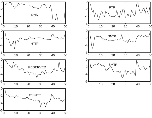
0 10 20 30 40 50 -6
-4 -2 0
DNS
0 10 20 30 40 50
-6 -4 -2 0
FTP
0 10 20 30 40 50
-6 -4 -2 0
HTTP
0 10 20 30 40 50
-6 -4 -2 0
NNTP
0 10 20 30 40 50
-6 -4 -2 0
RESERVED
0 10 20 30 40 50
-6 -4 -2 0
SMTP
0 10 20 30 40 50
-6 -4 -2 0
TELNET
Fig. 2: Plots of histograms (normalized and logged) for packet-size distributions (in 50 bins) of different applications.
From the plots, it can be observed that the packet size distributions for different applications display enough variations for a neural network to be trained to identify a given input as one of them. Thus the input to our neural network is a vector of 50 elements, each corresponding to a packet size bin mentioned above.
IV. CLASSIFICATION
A. Neural Network Architecture
As mentioned in the previous section, our aim is to classify a given input vector of dimension 50 into one of the 8 classes given in Table 1. For a problem of this dimensionality, a feed-forward backpropagation network with three layers would be appropriate. The input layer has 50 neurons corresponding to the dimensionality of input vectors. The output layer has 8 neurons, one representing each of our 8 classes. Hence, whenever the network is simulated, the ideal output should have a 1 at one of the 8 outputs, and 0’s at the remaining 7. The number of neurons in the hidden layer was selected based on the results of the following experiment.
2 4 6 8 10 12 14 16 18 20 10-5
10-4 10-3
10-2
10-1 MSE on set used for training
# of nodes in hidden layer ms
e
Test Set used for training Training Set used for training
2 4 6 8 10 12 14 16 18 20
0 0.005 0.01 0.015 0.02 0.025 0.03 0.035 0.04 0.045
MSE on set used for cross-validation
# of nodes in hidden layer ms
e
Training Set used for cross-validation Test Set used for cross-validation
2 4 6 8 10 12 14 16 18 20
0 5 10 15 20 25
# of misclassifications
# of hidden nodes #
of mi s cl.
Tested using Training Set Tested using Test Set
From the above study, it is seen that increasing the number of hidden nodes beyond 8 does not give significant improvement in performance. Hence, the number of hidden nodes for the neural network architecture used for classification was selected to be 8. The final neural net structure is shown in Fig. 4.
Fig. 4: Architecture of Neural Network used for classification
B. Classification Results
The results of classification are noted for two cases. In one, the neural network is trained using the Training Set, and the classification of Test Set is recorded. In the second, the reverse is done. The output of testing each input vector is a vector of dimension 8, where each element corresponds to one of the eight classes. The input vector is considered to be belonging to the class whose corresponding element is of the highest value in the vector.
The classification results for the first case are given in Table 2. It can be seen that we have a total of 3 misclassifications, or in other words, 98.44% accuracy. However, it should be noted that on a packet-count basis, the accuracy is higher – 99.31%. This is because all of HTTP and ‘All Other’ vectors are classified properly, and they account for a large part of the traffic mix as observed earlier.
TABLE 2
RESULTS CLASSIFICATION USING NEURAL NET– TRAINING USING TRAINING SET AND SIMULATING WITH TEST SET.
Actual
Experimental DNS FTP HTTP NNTP RES SMTP TEL All Other
DNS 24
FTP 23
HTTP 24 1
NNTP 1 23 1
RES 24
SMTP 23
TEL 24
All Other 24
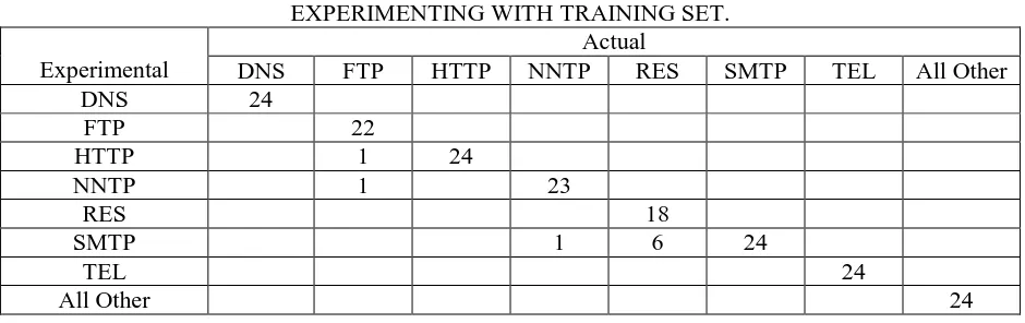
Similar classification results for the second case, i.e. training using Test Set and simulating using Training Set are given in Table 3. Here, we have a total of 4 misclassifications, i.e. 97.92% accuracy.
50
IW{1,1}
b{1}
8
IW{2,1}
b{2}
TABLE 3
RESULTS CLASSIFICATION USING NEURAL NET– TRAINING USING TEST SET AND SIMULATING WITH TRAINING SET.
Actual
Experimental DNS FTP HTTP NNTP RES SMTP TEL All Other
DNS 24
FTP 22
HTTP 24
NNTP 24
RES 24 1
SMTP 1 24 1
TEL 1 23
All Other 23
C. Classification Using Statistical Approach
We also did classification using the conventional statistical method of clustering. Here, in the first step clusters are formed using a data set, and then another set is classified using these clusters. We used the same input data as that used with the neural network approach, and did classification for both cases. The algorithm for determining the class to which a given test vector belongs is as below:
• Put the test vector into any one of the clusters
• Calculate the centroid of each cluster.
• Find the error for each cluster as the norm of the sum of distances of each member of a cluster from its respective centroid.
• Sum the errors for each of the clusters, or mathematically,
• total error =ÿÿ(norm(test vector – centroid))
• Repeat the same procedure by putting the test vector in each of the clusters.
• The test vector belongs to the cluster in which the total error comes out to be the least.
• Repeat the same experiment for all 192 (24x8) test vectors.
The results of the classification using this method are given in Tables 4 and 5. It can be seen that a total of 6 vectors are misclassified in the first case, and we get 96.88% accuracy in estimating the application to which a particular packet size distribution belongs. Similarly, for the second case we get an accuracy of 95.31%.
TABLE 4
RESULTS OF CLASSIFICATION – CLUSTERING USING TRAINING SET AND EXPERIMENTING WITH TEST SET.
Actual
Experimental DNS FTP HTTP NNTP RES SMTP TEL All Other
DNS 24
FTP 24
HTTP 24
NNTP 23
RES 24
SMTP 1 24 5
TEL 19
TABLE 5
RESULTS OF REVERSE CLASSIFICATION – CLUSTERING USING TEST SET AND EXPERIMENTING WITH TRAINING SET.
Actual
Experimental DNS FTP HTTP NNTP RES SMTP TEL All Other
DNS 24
FTP 22
HTTP 1 24
NNTP 1 23
RES 18
SMTP 1 6 24
TEL 24
All Other 24
V. CONCLUSION AND FUTURE WORK
We saw that using neural networks, we are able to classify major applications of Internet traffic. From that, it can be concluded that classification of Internet traffic using the features that are intrinsic characteristics of the packets, and features that cannot be spoofed so easily, is possible. This gives a completely new perspective of ‘implicit’ classification for differentiated services. The same classification can also be done using conventional statistics as indicated in the previous section. However, apart from giving slightly better classification, the neural network approach has its own benefits as explained in the introduction.
The work on classification in this manner is yet in its embryonic stage. The algorithms used have to be refined to attain real-time classification and adaptation to changing network dynamics. Also, it should be noted that we used ‘pure’ traffic for classification, i.e. the test vectors were purely that of the application, while the Internet traffic is a mixture of all applications. The further refinement in the algorithms should support classification in these practical conditions. The future work will have to distinctly identify the time-critical applications and include them in the study.
Along with this refinement of algorithm work, a parallel study is to be done of estimation and prediction, of traffic mix. Identifying the characteristics of applications that can help classify them is only the first step in the mixture estimation problem. And after estimation, we have to be able to predict the traffic mix for successive times. With the estimation and prediction problems resolved, methods for using this information in routers and schedulers can be developed.
REFERENCES
[1]. Mika Ilvesmaki, Marko Luoma, Raimo Kantola: Flow classification schemes in traffic-based multilayer IP switching – comparison between conventional and neural approach, Computer communications 21 (1998), pp. 1184-1194.
[2]. Fulu Li, Nabil Seddigh, Biswajit Nandy, Diego Malute: An empirical study of today’s Internet traffic for Differentiated Services IP QoS, Proceedings of ISCC 2000.
[3]. K. Glaffy, G. Miller, K. Thompson: The Nature of the Beast: Recent traffic measurements from an Internet Backbone, Proceedings of INET ’98, June 1998.
[5]. Dan Decasper, Zubin Dittia, Guru Parulkar, Bernhard Plattner: Router Plugins: A software architecture for next-generation routers, IEEE/ACM Transactions on Networking, Vol. 8, No. 1, February 2000.
[6]. Pankaj Gupta, Nick McKeown: Algorithms for Packet Classification, IEEE Network Magazine, March/April 2001, vol. 15, no. 2, pp. 24-32.
[7]. Mary L. Bailey, Burra Gopal, Michael A. Pagels, Larry L. Peterson, Prasenjit Sarkar: PathFinder: A pattern-based packet classifier, Proceedings of the First Symposium on Operating Systems Design and Implementation, pp. 115-123, November 1994.
[8]. S. Blake, D. Black, M. Carlson, E. Davies, Z. Wang, W. Wiess: An Architecture for Differentiated Services, RFC 2475.