ABSTRACT
NORMAN, MATTHEW ROSS. Characteristics-Based Methods for Efficient Parallel
Integration of the Atmospheric Dynamical Equations. (Under the direction of Dr. Fredrick H. M. Semazzi.)
The social need for realistic atmospheric simulation in weather prediction, climate change attribution, seasonal forecasting, and climate projection is great. To obtain realistic simulations, we need more physical processes included in the model with greater fidelity and finer spatial resolution. Spatial resolution primarily drives the need for computational resources because reducing the model grid spacing by a factor f requires f4times more computation (assuming 3-D refinement). This compute power comes from large parallel machines with 10,000s of separate nodes and accelerators such as graphics processing units (GPUs) making efficiency a complicated problem.
Efficiency parallel integration algorithms need low internode communication, minimal synchronization, large time steps, and clustered computation. To this end, we propose new characteristics-based methods for the atmospheric dynamical equations with these properties in mind. These schemes are capable of simulating at a large CFL time step in only one stage of computations, needing only one copy of the state variables. They are implemented in a 2-D non-hydrostatic compressible equation set in anx-z(horizontal-vertical) Cartesian plane to simulate buoyancy-driven flows such as rising thermals and internal gravity waves.
The schemes are implemented to run on CPU and multi-GPU architectures using Nvidia’s CUDA (Compute Unified Device Architecture) language to test relative efficiency. Even with-out memory tuning, the GPU code showed roughly 2.5x (5x) better performance per Watt. With optimization, this could increase by an order of magnitude.
polynomials and computes them on-the-fly. The advantage of on-the-fly calculations is a sig-nificant reduction in the volume of data communicated to and from the GPU’s slow global memory. In some cases, the runtime on GPUs of the same problem size cut in half because of this reduction in the amount of data communicated.
Regarding accuracy, a series of modifications were proposed and implemented in the hopes of improving accuracy. These included higher-order accurate trajectories and inclusion of the gravity source term in the characteristic variables and trajectories. When testing the compara-tive accuracies in a smooth gravity waves test case, the modifications showed from 10% to 20% improvement. Particularly, higher-order accurate trajectories yielded the best improvement for computational cost. It was found, however, that the amount of diffusion included in the scheme controlled the accuracy the most.
Overall, these schemes have proven viable for atmospheric simulation up to a CFL value near two when the hyperdiffusion is properly tuned. Compared to a three-stage scheme that sub-cycles fast waves twice per stage (for CFL = 2), this method requires one-sixth the synchro-nization points, one-third the communication, and one-half the memory requirements. Also, all computations are clustered into a single stage.
123435674896859AB397CDE762FC9DF4D85876D3437D674368FDFD627D6F927485D 3853D368F9
D
E36627D F99D!F43D
DC899746368FD98667CD6FD627D"43C367D#356DFD !F462D134F83D$6367D%8&74986D
8D34683D876DFD627D 47847769DF4D627D7477DFD
F56F4DFD28F9F2D
6F927485D$58757D
3782'D!F462D134F83D
()**
+,DB-.D
////////////////////////////// 40D#47C4851D20DE0D$73338
////////////////////////////// 40D 33523C43D0D!384
////////////////////////////// 40DE36627D0D34174
////////////////////////////// 40D2FD4F
Dedication
“Who knows a person’s thoughts except the spirit of that person, which is in him? So also
no one comprehends the thoughts of God except the Spirit of God. Now we have received not
the spirit of the world, but the Spirit who is from God, that we might understand the things
freely given us by God.” (1 Corinthians 2:11-12)
“Let no one deceive himself. If anyone among you thinks that he is wise in this age, let him
become a fool that he may become wise.” (1 Corinthians 3:18) Both quotations are from the
Holy Bible, English Standard Version, Copyright © 2001.
God, I dedicate this dissertation to you, knowing that my wisdom is foolishness. I take joy
in my neediness, knowing that your provision for me in Christ is better than my own. Had you
not saved me and were you not faithful to your promise to continue to save me daily, my heart
would remain selfish and futile, and I would never know the satisfaction of simply gazing on
you.
Thank you for sending Christ to take on himself the condemnation I’ve earned and instead
give me what I could not earn: adoption as your son, a promised inheritance to be with you
forever, and power over my depraved nature so I can do what is right. I ask that you would
continue your faithfulness to save me from my tendency to treasure everything but you. Fix
my gaze on your nature, goodness, and perfection, and satisfy me by your grace in Christ.
Shannon, you are the most important person to me on this Earth, and as I promised from the
beginning that you always would be, I promise still now that you will continue to be. I dedicate
this to you secondly because of your sacrifices and labor in enduring doctoral studies with me.
I want to honor you as a beautiful and Godly wife whom by God’s grace I value above myself
Biography
Matthew Ross Norman was born in 1983 and grew up in Greenville, NC during grade school,
middle school, and high school with an interest in mathematics and physics. Afterward, he
attended North Carolina State University graduating with honors in May of 2006 with a B.S. in
meteorology, a B.S. in computer science, and a minor in mathematics. He then began graduate
studies at North Carolina State University for a M.S. degree in atmospheric science. In 2008,
he received his M.S. degree, and he then received the Department of Energy Computational
Science Graduate Fellowship which funded doctoral studies for two and a half years until the
Acknowledgments
I would like to acknowledge my committee with great gratitude. I count myself very fortunate
to have this committee because I have learned from all of them whether as an instructor or as a
supervisor. Particularly, Dr. Semazzi has been an excellent advisor and began the connections
that led me to the field of computational science, beginning my interests in semi-Lagrangian
methods. Also, much of this material was performed under the supervision and with the help
and aid of Dr. Nair at the National Center for Atmospheric Research. I learned a great deal
from numerical modeling courses taught by Dr. Luo and Dr. Parker.
I would also like to acknowledge generous funding by the Department of Energy
Computa-tional Science Graduate Fellowship. Also, I would like to thank the Advanced Study Program
at the National Center for Atmospheric Research for funding a 10-month visit during which I
Table of Contents
List of Tables . . . ix
List of Figures . . . x
Chapter 1 Motivation . . . 1
1.1 Society’s Need For Atmospheric Models . . . 1
1.2 Description of Atmospheric Dynamical Cores . . . 2
1.3 Meeting Computational Demands . . . 7
1.3.1 Notions of Scaling . . . 9
1.3.1.1 Strong scaling and Amdahl’s Law . . . 9
1.3.1.2 Weak Scaling and Gustafson’s Law . . . 13
1.3.2 Efficiency On Distributed Memory GPU-Based Machines . . . 14
1.4 Purpose Statement . . . 16
Chapter 2 Review and Background Material . . . 17
2.1 The Equation Set And Physical Bases . . . 17
2.1.1 2-D Stratified Compressible Non-Hydrostatic Atmospheric Model . . . 18
2.1.2 Characteristic Theory . . . 20
2.1.3 Primitive Variable Formulation . . . 26
2.2 Integrating the Equations . . . 28
2.2.1 Spatio-temporal Integration . . . 28
2.2.1.1 Spatial Categorizations . . . 28
Finite Difference . . . 29
Finite Volume . . . 29
2.2.1.2 Temporal Categorizations . . . 33
Fully Discrete and Semi-Discrete . . . 33
Multi-Stage and Multi-Step . . . 34
Implicit and Explicit . . . 35
Upwind and Central . . . 38
Eulerian and Lagrangian . . . 39
2.2.2 Operator Splitting . . . 40
2.2.3 Summary Of Categorizations Chosen Herein . . . 43
2.2.4 Time-Explicit Fully Discrete Finite Volume Framework . . . 44
2.2.5 Discontinuous Flux Evaluations . . . 45
2.2.6 Approximate Riemann Solvers . . . 47
2.2.6.1 Flux Difference Splitting . . . 48
2.2.6.2 An Alternative Approach . . . 49
2.2.7 Reconstruction . . . 50
2.2.7.1 High-Order Accurate Reconstruction . . . 51
2.2.7.2 Polynomial Interpolation . . . 52
2.2.7.3 Reconstructing Derivative Information . . . 55
2.2.7.4 Total Variation, Monotonicity, and Oscillations . . . 55
2.2.7.5 Non-Oscillatory Reconstructions . . . 57
2.2.7.6 Weighted Essentially Non-Oscillatory (WENO) Interpolants . 58 Chapter 3 Mathematical Formulations: New Characteristics-Based Methods . . 60
3.1 Original Formulation: The Flux-Based Characteristic Semi-Lagrangian Method 61 3.1.1 Boundary Conditions . . . 63
3.1.2 Hydrostatic Balance and Solid Wall Boundary Conditions . . . 63
3.1.4 Flux Computation Summary . . . 68
3.2 Analysis of the Original FBCSL Formulation . . . 69
3.2.1 Communication Needs . . . 69
3.2.2 Memory Requirements . . . 72
3.2.3 Assumptions and Inaccuracies . . . 72
3.2.4 Synchronization, Compute Intensity, and Local Memory . . . 73
3.3 Modifications In This Study . . . 74
3.3.1 Modifying the Interpolation of the Original Formulation . . . 74
3.3.1.1 On the Fly Interpolation . . . 75
3.3.1.2 Hyperdiffusion . . . 76
3.3.2 Higher-Order Accurate Trajectories . . . 80
3.3.3 Characteristic Handling of the Gravity Source Term . . . 82
3.3.3.1 Inclusion of Gravity Source Term in the Characteristics . . . 86
State Variable-Based . . . 86
Flux-Based . . . 87
Affecting Trajectories . . . 89
3.3.4 Algorithmic Handling of Characteristic Source Terms . . . 90
Chapter 4 Numerical Results and Discussion . . . 91
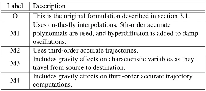
4.1 Model Formulations and Test Cases . . . 91
4.1.1 Model Formulations . . . 91
4.1.2 Test Cases . . . 92
Constant Potential Temperature . . . 93
Constant Brunt-Vaisala frequency . . . 93
4.1.2.1 Convective Thermal . . . 94
4.1.2.3 Non-Hydrostatic Internal Gravity Waves . . . 95
4.1.2.4 Bubble Collision . . . 96
4.2 Results For The Original Formulation . . . 96
4.2.1 Convective Thermal . . . 97
4.2.2 Straka Density Current . . . 100
4.2.3 Non-Hydrostatic Internal Gravity Waves . . . 105
4.3 Implementing A Multi-GPU Code . . . 111
4.4 Complexity and Runtimes of Model Modifications . . . 115
4.4.1 Computational Complexities . . . 115
4.4.1.1 Original Formulation . . . 116
4.4.1.2 M1: On The Fly Interpolation . . . 117
4.4.2 Runtimes Of The Model Formulations . . . 118
4.4.2.1 GPU Set-up Choices . . . 118
4.4.3 Discussion of Runtimes . . . 120
4.5 Quantitative Accuracy Comparison Among Model Formulations . . . 123
4.5.1 Discussion . . . 127
4.5.2 Damping and the Tuning of Hyperdiffusion . . . 128
Chapter 5 Concluding Remarks and Future Directions . . . 135
5.1 Conclusions . . . 135
5.2 Further Improvements . . . 137
5.3 Future Extension to Other Models . . . 138
5.3.1 Global, 3-D, Energy Conserving Non-Hydrostatic Model . . . 139
List of Tables
Table 4.1 List of model formulations for the 2-D non-hydrostatic model. . . 92
Table 4.2 Maximum and minimum potential temperature perturbation at 900
sec-onds for the Straka density test case with diffusion. . . 101
Table 4.3 Error norms in the potential temperature field compared to 25m results. . 105
Table 4.4 Runtimes in seconds of the original and M1 formulation in simulating
the convective thermal test case for 100 seconds. . . 121
Table 4.5 Error norms for formulations O, M1, M12, M13, and M123.
Formu-lations M124 and M1234 are omitted because including gravity forcing
within the trajectories had negligible effects on the error norms such that
List of Figures
Figure 1.1 Plots of maximum speed-up with and without communication overhead
according to Amdahl’s law of strong scaling. All axes are log scale. . . . 11
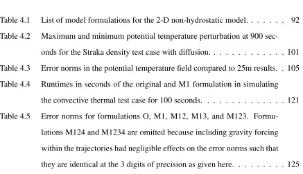
Figure 1.2 Plots of maximum speed-up with and without communication overhead
according to Gustafson’s law of weak scaling. All axes are log scale. . . 15
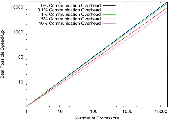
Figure 3.1 Schematic of the process for computing time-averaged characteristic
variables with CFL=1.5 for the interface with a red dashed line. The blue
arrow is the upwind trajectory, and the violet dashed line is the departure
location. Dark green circles denote quadrature points at which the flux
is calculated from reconstructions to compute characteristic variables at
locationsxm,p. Note separate quadrature within each cell. . . 69
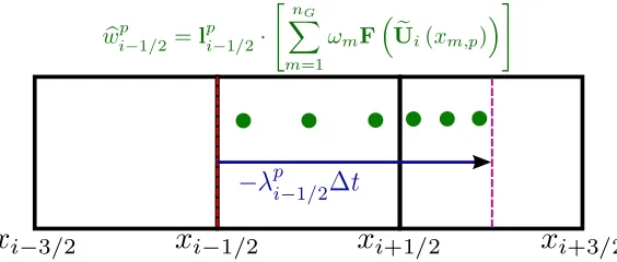
Figure 3.2 Plots of the amplitude fraction over range spatial scales after applying a
second-order accurate hyperdiffusion of orders ranging from 2 to 8 with
a forward Euler time step. . . 79
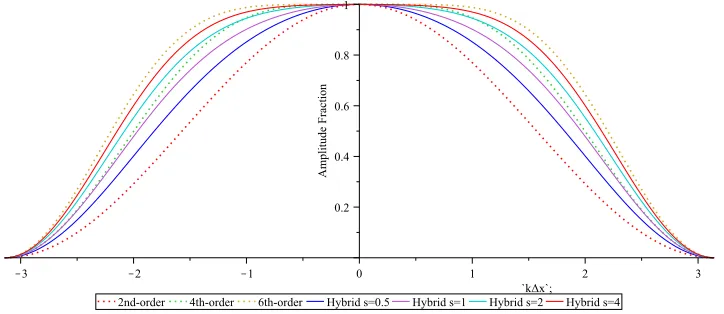
Figure 3.3 Plots of the amplitude fraction over range spatial scales after applying
standard hyperdiffusion and hybrid hyperdiffusion over a range of scale
separation parameters s. For all standard hyperdiffusion plots, β =1, and for all hybrid hyperdiffusion plots,db=1. . . 80
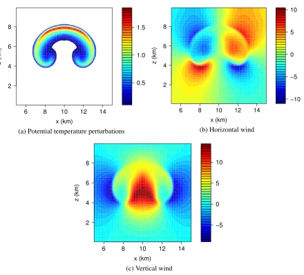
Figure 4.1 Plots for the convective thermal test case with a 125 m grid spacing after
1,000 sec of simulation. x- andy-axes are in km, potential temperature
Figure 4.2 Domain maximum potential temperature and vertical wind traces for the
convective thermal test case over a range of grid spacings.x-axis is time
in seconds andy-axis isK for potential temperature trace and ms−1for
vertical wind trace. . . 99
Figure 4.3 Plots for the convective thermal test case with a 125 m grid spacing after
1,000 sec of simulation with a CFL number of 1.96.x- andy-axes are in
km, potential temperature perturbations are inK. . . 99
Figure 4.4 Plot of the kinetic energy power at a given wavenumber for the rising
thermal test case over a broad range of grid spacings. . . 101
Figure 4.5 Plots for the Straka density current test case after 900 seconds with
dif-fusion for grid spacings ranging from 25m to 400m. x- andy-axes are in
km and potential temperature perturbations are inK. . . 102
Figure 4.6 Contours of potential temperature perturbation for the Straka density
current test case without explicit numerical viscosity after 900 seconds
with a grid spacing of 50m. x- andy-axes are in km and potential
tem-perature perturbations are inK. For visual clarity, they are plotted with
half the number of contours as Fig. 4.5. . . 104
Figure 4.7 Plots for the internal gravity waves test case after 3,000 seconds with a
range of grid spacings with CFLmax=0.99. ∆x=10∆zfor all
simula-tions. The x- andy-axes are in km and potential temperature
perturba-tions are inK. . . 106
Figure 4.8 Plot of potential temperature perturbations along the line z=5km for
the internal gravity waves test case after 3,000 seconds with a range of
grid spacings. ∆x=10∆zfor all simulations. The x-axis is in km and
Figure 4.9 Log-log plot of potential temperature errors (increasing upward) as a
function of grid spacing (decreasing to the right). We used the 25m run
to represent the exact answer and add lines whose slopes show visually
the order of convergence. . . 107
Figure 4.10 Plots for the internal gravity waves test case after 3,000 seconds with a
maximum CFL number of 2. ∆x=10∆z=1,000 m. Thex- andy-axes are in km and potential temperature perturbations are inK. . . 108
Figure 4.11 Plots for the internal gravity waves test case after 3,000 seconds with a
maximum CFL number of 3. ∆x=10∆z=1,000 m. Thex- andy-axes are in km and potential temperature perturbations are inK. . . 109
Figure 4.12 Plots for the internal gravity waves test case after 3,000 seconds with a
maximum CFL number of 4. ∆x=10∆z=1,000 m. Thex- andy-axes are in km and potential temperature perturbations are inK. . . 110
Figure 4.13 Image and Schematic of the Nvidia GF100 GPU chip. The image can be
found athttp://benchmarkreviews.com/images/reviews/processor/
NVIDIA_Fermi/nvidia-fermi-gf100-graphics-processor-high-resolution.
jpg(December, 2010), and the schematic can be found athttp://www.
thinkdigit.com/FCKeditor/uploads/GF100.png(December, 2010). 118
Figure 4.14 Visual comparison of accuracy via a bar plot of L1, L2, and L∞ error
norms for the gravity waves test case after 3,000 seconds. Plots are
scaled as mentioned in the subfigure captions for visual clarity. . . 126
Figure 4.15 Kinetic energy power spectra for the original formulation (labeled “WENO”)
and for the M1 modification (labeled “Hyper Diffusion”) at varying CFL
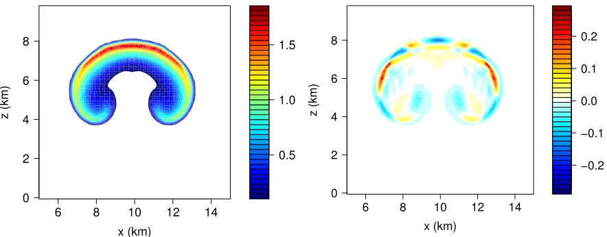
Figure 4.16 Visual comparison of various diffusion mechanisms and levels for the
rising thermal test case after 1,000 seconds. The top line is the
orig-inal formulation with WENO interpolants. The bottom three lines are
the M1 modification with varying damping coefficients as shown. All
hyperdiffusion damping scales for M1 runs are set tos=1.5. . . 131 Figure 4.17 Potential temperature contours of the rising thermal test case after 1,000
seconds with the M1 formulation with varying hyperdiffusion damping
coefficients. . . 132
Figure 4.18 Visual comparison of various diffusion mechanisms and levels for the
Straka density test case after 900s. The top line is the original
formula-tion with WENO interpolants. The bottom three lines are the M1
modi-fication with varying damping coefficients as shown. All hyperdiffusion
damping scales for M1 runs are set to s=1.5. Missing figures indi-cate inability to run stably with the specified hyperdiffusion damping
parameter. . . 133
Figure 4.19 Visual comparison of Straka density currents after 900 seconds with the
originally specified diffusion of 75 m2s−1 simulated with the M1
Chapter 1
Motivation
1.1
Society’s Need For Atmospheric Models
There are many socioeconomic applications of atmospheric modeling including weather
fore-casting, climate projections, attribution of climate changes, and seasonal to decadal
predic-tions. All applications share the ever-increasing hunger for more realistic simulations, whether
through increases in spatial resolution or inclusion / improvement of more physical
phenom-ena, e.g. cloud schemes (to simulate mesoscale structure), aerosol-cloud interactions, and other
atmospheric chemistry.
Socially and politically, the impacts of climate changes whether due to anthropogenic
influ-ences or natural internal variability are immense. Particularly, as changes in time-mean climate
regimes alias onto seasonal and annual cycles, water budget changes alone may relocate
en-tire regions if resources fall below the ability to support current populations. Also, the ability
to forecast seasonally averaged properties such as precipitation, temperatures, growing degree
days, and extreme event frequency better than climatology (e.g. for either irrigating or
dig-ging trenches responding to below or above normal precipitation respectively) would enable
Though the inclusion of more spatial scales and more phenomena in modeling invariably
increases the amount of uncertainty, one can more confidently approximate the range of future
climate regimes, including both the bounds and the probability distribution within. With
in-crease uncertainty one would be unwise not to also inin-crease the number of ensembles to ensure
as large of a sampling rate as is computationally feasible so that at least our confidence in what
we think we know can increase.
All of this requires computational resources as well as models that are well-suited to run
on the available resources as they evolve. This is the ultimate goal toward which this study
contributes: devising numerical modeling algorithms with the computational hardware in mind
to unlock the immense resources available to help answer the pressing questions of science and
society. Specifically, we will be working on one part of atmospheric models which tends to set
the stage for the rest of the model’s computational efficiency as it defines the resolvable spatial
scales in simulation.
The next section defines this component of atmospheric models, how it is different from
the rest of the model, and the role it plays in the overall coupled simulation in which each
component’s individual realism and interaction with the other components is paramount to
produce a sound overall simulation.
1.2
Description of Atmospheric Dynamical Cores
Atmospheric models are ideologically (and practically) split into two components: (1) the
dynamical core (hereafter, dycore) and (2) the physics packages. The dycore integrates the dry
(only meaning no precipitants or clouds, water vapor is still included) fluid dynamical equations
of the stratified atmosphere in a rotating reference frame on the sphere (Earth’s surface) as
well as transports quantities used by the physics packages. It deals with Coriolis force, the
acceleration), and all resolved dynamics that occur in this context [2].
The physics packages include everything that is not resolved by the dycore and can
gen-erally be broken into two parts. First, the physics includes all phenomena not resolved by the
dycore due to discretization because they occur on smaller spatial or temporal scales. This
would include phenomena such as dry convective adjustment, gravity wave drag, and eddy
dis-sipation. Second, the physics includes all phenomena not resolved at all by the dynamical core
equation set such as moist physics, radiative forcings, biogeochemical cycles and feedbacks,
and couplings with other model components. Another aspect of modeling the full climate
sys-tem is the coupling of multiple physical components of the climate syssys-tem, mainly grouped
into four models: atmosphere, ocean, land surface, and cryosphere [3]. These are treated in
similar manner to the physics as far as the dycore is concerned.
It would be wrong to assume to any extent that the dycore and physics are actually separate
or that one is more important than the other. Of course, in reality we have a set of extremely
complex and non-linear differential / integral relationships closed with empirically /
stochas-tically derived closures which evolve together continuously in space and time. Since they are
separate in the discrete models usually in both development and implementation, one must
re-spect the spatio-temporal scales of coupling as well as properly tune the physics parameters to
the various properties of the dycore integration.
Unfortunately, this tuning process is extremely difficult and necessarily relies upon the
ex-pertise and scientific intuition of well-experienced senior modelers. One cannot simply tune
parameters of many of the model components to physical experiments in many cases for two
reasons. First, physical experiments may not be possible for many of the closure models
be-cause the parameters arise out of a mathematical model and perhaps not a physically realizable
quantity. Second, due to discretization errors, when components interact, many of the scales
of interaction are severely altered, and many of the quantities do not retain physically
parameters in complex coupled models, tuning physics packages and dycores to one another is
both individual to the schemes and components used and is not necessarily a physically-based
process.
This study is concerned only with the dycore, and thus the discussion of physical packages
and tuning will be left to the above paragraphs. The dycore integrates a set of partial
differ-ential equations of a special form known as conservation laws (though many models operate
on altered equation sets that are not in conservation form). Conservation laws relate the time
rate of change of a physical quantity to the spatial divergence of some physically relevant flux
which is a function of that quantity. Natural to the name, the physical quantities in question
are conserved (meaning the global integral of the quantity must not change in the absence of
source terms). One should think of the flux as a function linking the local spatial distribution
of the conserved quantity to the local temporal evolution.
For example, consider the one-dimensional transport of mass per unit volume (i.e. density):
∂tρ+∂x(ρu) =0. (1.1)
The change in density,ρ, in time at a given point is related to gradient of the flux,ρu, at that point whereuis the wind velocity. If the gradient ofρuis large in the local surroundings, then
ρ will change very quickly, but if
dρu
dx =0 (1.2)
it will not change at all.
This makes physical sense. Suppose instead we considered
whereT is temperature. Supposingu≡uis uniform in space, the equation becomes:
∂tT+u∂xT =0. (1.4)
The equation shows two ways of having the temperature change quickly at a location. Even if
temperature is changing slow in space, if the wind is very strong, then the local temperature will
change quickly. Secondly, even if the wind is weak, if the temperature changes very strongly
with space in the local surroundings, the local temperature change will be large. Therefore, the
product of the two has a natural interpretation. Not all conservation laws are so intuitive, but
this provides a simple example to see how the flux relates spatial surroundings with the local
change in time.
The dycore is designed to conserve mass, momentum, and a thermodynamic variable (often
energy, but sometimes a quantity known as potential temperature) [4]. Note that some dycores
rather conserve wind instead of momentum though the modern trend is to conserve
momen-tum. Along with this, dycores also conserve all of the physical quantities used by the physics
packages (which are called “tracers” in short) in a form similar to mass conservation (i.e. they
are evolved by the wind). For instance, to conserve a mixing ratio of water vaporq, the tracer
transport conservation law would be:
∂t(ρq) +∂x(ρuq) =0. (1.5)
In micro-scale / cloud-scale dycores, the only thing added to this set of equations is a
grav-ity source term to the vertical momentum conservation law. Though seemingly only a small
change, this addition changes the entire character of the flow because stratified fluids (where
density changes by orders of magnitude over the vertical column) behave much differently than
gradient force and gravity, known as hydrostatic balance. Also, phenomena such as gravity
waves and unstable convection arise out of stratification [5]. Unstratified fluids (i.e. much
smaller vertical length scales) undergo gravity acceleration largely as a whole, meaning the
effect of gravity can often be ignored as a source of interesting dynamics.
As the horizontal spatial scale increases, other processes become important such as
Corio-lis force and Earth’s curvature. In these cases, equation sets must take into account the Earth’s
curvature, typically through some metric transformation into a more convenient computational
space. Also, the momentum equations are affected by Coriolis forcing (an apparent force
arising out of integrating in a rotating reference frame). Technically, the vertical momentum
equation should include a Coriolis forcing term, but by scale analysis, this term is often
de-clared insignificant and left out of the simulation. Therefore, Coriolis becomes a dominant
player but only in the horizontal dynamics.
As with gravity to the vertical momentum equation, Coriolis completely changes the
char-acter of the horizontal flow. Instead of fluid flowing from high pressure to low pressure, in
large scales, the fluid rather rotates around the extrema in pressure in the mid- to high-latitudes.
This is described by the well-known geostrophic balance between Coriolis forcing and
pres-sure gradients. [6] Because of geostrophic balance, horizontal dynamics in the atmosphere are
dominated by non-divergent flow regimes. With weak Coriolis forcing in the tropics, divergent
flows again become more significant.
Geostrophic and hydrostatic balances dominate the atmospheric state, and an effective
dy-core must respect the intricate interplays between fluxes and these important source terms.
More to the point, an effective dycore must accurately resolve the perturbations from these
balances which form the motions of interest for atmospheric dynamics. Given a grid spacing,
it is desired that a dycore resolve the smallest scales possible meaning the lowest amount of
1.3
Meeting Computational Demands
Atmospheric models increase in realism (in a broad sense) by the inclusion of more physical
phenomena, the improvement of existing simulated phenomena, and the increase of spatial
resolution. These improvements are fueled by increases in computational power, meaning that
the ability of the model to use the latest advanced hardware directly determines the simulating
capabilities. In the past, computing power increased mainly on single nodes through various
means including: faster chips, instruction level parallelism (pipelining, speculative execution,
Streaming Scalar Extensions, etc), and shared memory parallelism. Speed-up on these
ma-chines was nearly automatic, and together with algorithmic advances such as semi-implicit,
semi-Lagrangian (SISL) and explicit sub-cycled models (to be discussed in section 2.2), great
advances in model efficiency and thus realism occurred.
Eventually, the price of these vector-type machines was undercut by a popular design of
using cheap commodity hardware units and linking them with network interconnect. These
machines are called distributed memory because memory is now distributed among various
nodes, and data is communicated over a network. This brought a new constraint to the table:
communication cost. The algorithms well-suited for shared memory parallelism required
sig-nificant amounts of communication over distributed memory machines and no longer scaled
efficiently. Explicit sub-cycled methods require less communication than do SISL methods, so
they attained better parallel efficiency on distributed memory machines.
Today, the amount of distributed memory parallelism is enormous. For instance, Jaguar
1 from Oak Ridge National Laboratory (ORNL) has 18,000 nodes, each with two hex-core
processors each (about 250,000 processing cores in all). Communication across 18,000 nodes
takes a lot of time, and it is best to do this as little and least often as possible. New
algo-rithms (specifically of the finite element type) have been developed to deal with this problem,
communicating very small amounts of data per time step. The spectral element method in
particular has shown great success for the atmosphere simulating at a grid spacing of about
14km at reasonable model throughputs (almost 5 simulated years per day (SYPD) [personal
communication with Dr. Mark Taylor, Sandia National Laboratory, 2010].
The new problem is that these commodity machines are using up too much power. For
instance, ORNL’s Jaguar uses 7 Megawatts to achieve 2 Petaflops2 (2 quadrillion operations
per second) of computational processing. To reach exascale (a roughly 500 fold increase),
this means around 5 Gigawatts of power will be consumed by the machine if it scales linearly
(i.e. in a “perfect world”). Regardless, a few Gigawatts is the total power output of many
power plants. Therefore, we need a paradigm change. On this note various accelerators such
as the IBM Cell Broadband Engine (Cell BE) chips and Graphics Processing Units (GPUs) are
entering the supercomputing market at an opportune time.
GPUs are used for computer gaming, and they mainly handle mapping graphical textures
to game surfaces as well as much of the game physics. They are constructed for applications
that follow the “single instruction multiple data” or SIMD paradigm, meaning they are good
at performing the same operation on lots of different data. Luckily for modelers, atmospheric
modeling fits this bill pretty well. Physically, one could think of GPUs as a collection of
multi-processors where multi-processors can coordinate within a multiprocessor but not between separate
multiprocessors. In some ways, it marks the return to the general vector machine paradigms
with some added constraints for efficiency (discussed later). The difference is that GPU
tech-nology is driven by the gaming market, making these “desktop supercomputers” highly
acces-sible cost-wise.
GPUs (or similar accelerators) have already been included in many supercomputers. As a
case in point, China’s new “Dawning Nebulae” machine is built using GPUs and falls in as the
world’s fastest computer (up to December 2010 so far) and also one of the most energy efficient
2
3 4. Given the changes that have already occurred in supercomputing and the changes that are
likely to occur very soon, atmospheric models have a long way to go before they will run well
on these new machines. This is where the present research fits in: to design an integration
algorithm well-suited for these distributed memory accelerator-based platforms.
1.3.1
Notions of Scaling
When someone mentions an application “scaling” well, this can carry a variety of meanings.
Here, we will define some of those notions.
1.3.1.1 Strong scaling and Amdahl’s Law
Suppose we have an atmospheric model running at 1◦ resolution globally and we want to
get the model running as fast as possible at that resolution by spreading it among as many
processors as possible. This is what is known as “strong scaling”: reducing the runtime of a
fixed problem size as much as possible by increasing the number of processing elements used.
More specifically, linear (or perfect) strong scaling means that a process that takest time in
serial will taket/ptime on pprocessors. Strong scaling is nearly always sub-linear because of communication latencies, parts of the code that cannot be parallelized, and portions of code
that must be duplicated among more than one process.
Amdahl’s law [7] sets the maximum scalability given the ideal scenario of instant internode
communication based on the proportion of the code that is parallelizable. Suppose p is the
parallel proportion of the code. Thus, the serial proportion, s, is s=1−p. Assume a serial
runtime,ts. If the parallel portion is broken inton pieces performed perfectly in parallel, this
3http://www.top500.org/December, 2010 4
code will have a parallel runtime,tp, of
tp= pts
n +sts (1.6)
time. Speed-up,Sis defined as the ratio of the serial runtime to the parallel runtime: S=ts/tp.
This gives a speed-up (in an ideal case) of:
S= ptsts
n +sts
= p 1
n+1−p
. (1.7)
Another useful metric is efficiency which gives the average percent use of each processor:
E=S/n. Fig. 1.1a shows the best possible speed-up and efficiency for a range of parallel
pro-portions, p, over a range of processor numbers,n. As one increases the number of processors
to infinity, the maximum speed-up is defined bySmax=1/s.
This means that a code that is 99% parallelizable even with infinite processors working
will get a speed-up of only 100 via strong scaling even in a perfect world communication
wise. In fact, the situation is much worse than this. Assume we have a log2ncommunication
time associated with each parallel piece of work (a very optimistic assumption on network
topology). The parallel time would now be
tp= pts
n +cptslog2n+sts (1.8)
wherecis the communication time between two nodes as the overhead for each parallel task.
For instancec=0.1 would indicate that a parallel node will spend 10% communicating data for every block of execution it performs (a 10% communication overhead). This gives a new
speed-up of:
S= p 1
n+cplog2n+1−p
1 10 100 1000 10000
1 10 100 1000 10000
Best Possible Speed-Up
Number of Processors 100% Parallelizable
99.9% Parallelizable 99% Parallelizable 95% Parallelizable 80% Parallelizable
(a) Maximum speed-up for different parallelizable proportions assuming no communication overhead.
1 10 100 1000 10000
1 10 100 1000 10000
Best Possible Speed-Up
Number of Processors 0% Communication Overhead 0.1% Communication Overhead 1% Communication Overhead 5% Communication Overhead 10% Communication Overhead
(b) Maximum speed-up for 100% parallelizable problem with varying com-munication overheads.
Note that this asymptotes to zero as n→∞. Plots of the maximum speed-up over a range
of communication overheads assuming a 100% parallelizable problem are given in Fig. 1.1b.
At this point, there is a global maximum in speed-up after which the overall runtime even
degrades.
To discuss the merits of reducing communication on very large systems, we can introduce
two new variables: fcmis the factor by which communication is reduced, and fcpis the factor
by which computation is increased (i.e. serial time is increased). Also, to accommodate more
realistic assumptions on network topology, we consider a√ncommunication model. The new
model mimicking these effects under Amdahl’s scaling is:
S∗= 1
fcp
1
p n+
cp√n
fcm +1−p
. (1.10)
The speed-up over an the original model associated with cutting communication can then
be given by: S∗/S. Suppose p=0.99, n=20,000, andc=0.01. If the amount of overall computation remains the same (fcp=1) and the communication cost is cut to a third (fcm=3),
the speed-up associated with reducing communication (S∗/S) is 2.10. Even if the amount of computation increases by 50% (1.5), the speed-up associated with reducing communication is
still 1.4.
Though this model is far from robust (at least the parameter should be tuned to measured
values), it does still demonstrate the “flops for free” mentality that is growing in the High
Per-formance Computing community. In this mentality, if communication dominates the overall
runtime, one can increase the amount of computation significantly with relatively little overall
runtime penalty. Moreso, if additional computation can decrease the amount of
1.3.1.2 Weak Scaling and Gustafson’s Law
Now, suppose it take one day to simulate five model years at 1◦resolution. If we wish to solve
bigger problems in the same amount of time, refining the grid spacing and distributing among
more processors at the same time. This is known as “weak scaling”: scaling the problem size
with the number of processors at equal rates for a fixed total runtime. Constant (or perfect)
weak scaling means that ifngrid points are simulated in a given runtimet, then pngrid points
can also be simulated in timet when distributed over p processors. This is the more realistic
scenario of the two because we always want more information in the same amount of time.
Gustafson’s law [8] sets the maximum scalability assuming the problem size is increased
at the same rate as the number of processors. Assume that the execution time on a parallel
computer is split into a serial time,s, and a parallel time, p′ (noting that p′ is not the same as
section 1.3.1.1). Also assume for simplicity that the total time takes one unit: tp=s+p
′ =1.
This problem on a serial computer with no parallel overhead (i.e. perfect world), would be
ts=s+np′. Since we assumed the parallel time was 1, then we can say p′=1−sand
S= ts
tp
=s+n(1−s). (1.11)
Plots of this scaling relation are given in Fig. 1.2a. Clearly, the speed-up is much closer to
linear when the problem is scaled along with the number of processors.
Using the same communication model as before, the parallel time would become:tp=s+
p′(1+clog2n) =1. Then, the serial time is:ts=s+np
′
. Now we can set: p′= (1−s)/(1+clog2n). This gives a final scaled speed-up of:
S=s+ n(1−s)
1+clog2n. (1.12)
com-pared to Amdahl’s law. This scaling relationship assumes that the serial time is independent
of the number of processors which usually is not the case. Also, the parallel communication
overhead is typically much more stringent than the log profile used for both of these scaling
laws.
1.3.2
Efficiency On Distributed Memory GPU-Based Machines
The initial goal of this dissertation research at inception was to develop methods efficient on
large CPU-based distributed memory architectures. However, given the overwhelming
adop-tion of GPUs in supercomputing, we have added on GPU efficiency as another constraint for
the methods herein. GPUs add additional constraints to those already given by past distributed
memory architectures, so we will begin with traditional efficiency constraints. Low
commu-nication requirements are key for distributed memory machines because of how costly it is to
send data over network. Spectral element and discontinuous Galerkin methods have shown the
merit in lowering communication. Also, one cannot forget the traditional wisdom that an
ex-pensive scheme (flop-wise) must have a payoff (spatial resolution or larger time step perhaps)
for the extra flops.
As for GPUs, they are a collection of multi-processors with 8-16 processors each. One
launches a program on a GPU as a very large collection of threads (we have used over 10
mil-lion), and they coordinate together in “blocks” of up to 512 threads per block. Blocks are a
soft-ware abstraction which physically maps to a multi-processor on the GPU device. Each block
has about 16 - 32 thousand registers (the fastest on-chip memory) to split up among threads
and about 16 - 48 Kb of shared memory (another source of very fast memory) to share between
the threads. These are the biggest efficiency constraints because the main “global” memory
(typically between 1-6 Gb) is very slow. Threads must have low enough local memory
1 10 100 1000 10000
1 10 100 1000 10000
Best Possible Speed-Up
Number of Processors 100% Parallelizable
99.9% Parallelizable 99% Parallelizable 95% Parallelizable 80% Parallelizable
(a) Maximum speed-up for different parallelizable proportions assuming no communication overhead.
1 10 100 1000 10000
1 10 100 1000 10000
Best Possible Speed-Up
Number of Processors 0% Communication Overhead 0.1% Communication Overhead 1% Communication Overhead 5% Communication Overhead 10% Communication Overhead
(b) Maximum speed-up for 100% parallelizable problem with varying com-munication overheads.
reuse of these values in the integration algorithm to warrant the use of local memory.
Also, threads must be “compute intensive” meaning they do a lot of computation with data
grabbed from global memory. One of the tricks GPUs use is to switch between threads when
they request global memory and try to do useful work while waiting on the memory access.
This is a form of pipelining which almost entirely erases the amount of time it takes to access
global memory when there is enough available work either by large compute intensity or a
large number of threads. But it is only effective if one uses local fast memory to reuse data
taken from global memory and if the data retrieved feeds a lot of computation. In this sense,
one should actually try to increase the flop count per time step, but only if the extra operations
add to the spatial resolution. This gives higher-order accurate methods an advantage.
1.4
Purpose Statement
The purposes of this dissertation are to discuss the issues plaguing the efficient use of modern
supercomputing for atmospheric simulation, to develop characteristics-based theory for low
communication, large time step, and compute intensive integration, to discuss how the new
methods address these traditional computational problems, and to test this theory via
Chapter 2
Review and Background Material
This chapter is intended to provide the building blocks for the theory and motivation for the
next chapter on newly contributed characteristics-based methods. Though some of the content
is necessarily segmented, we try to enforce a flow to the ideas. Whenever possible, as various
material is introduced, it will be linked to the goals of this study to demonstrate why it is or is
not used for integration herein.
2.1
The Equation Set And Physical Bases
The equation set used in this study is a 2-D stratified compressible non-hydrostatic equation
set simulating buoyancy-driven dynamics in anx-z(horizontal-vertical) rectangular Cartesian
plane. This equation set conserves mass, momentum, and potential temperature with a gravity
source term. This is chosen because it contains minimal source terms (gravity only) and allows
a broad range of smooth and non-smooth flow for testing the stability and viability of the
methods introduced herein. In reality these methods are intended mainly for the horizontal
domain wherein the vertical dimension would likely be handled by an implicit method. But it
implement this equation set in rectangular Cartesian geometry.
2.1.1
2-D Stratified Compressible Non-Hydrostatic Atmospheric Model
The dycore, as mentioned in Section 1.2, must integrate the gas phase equations of fluid
dy-namics for a stratified fluid on a rotating sphere as well as transport the physics tracers. To
keep this study contained, we will only consider the integration of a stratified fluid in two
di-mensions. This is intended mainly as a prototype testbed. The equations are described by
conservation laws which conserve mass, momentum, and a thermodynamic variable according
to various physical principles guiding how their flux functions should be specified. Mass for
instance is guided by continuity dictating that it may not be created or destroyed. Momentum
arises from Newton’s second law of motion stating that a particle’s acceleration is given by
the sum of forces acting upon it. The thermodynamic equation is governed by the first law of
thermodynamics stating the conservation of energy and its transitions among internal energy,
potential energy, and work.
The conservation laws used in this study conserve mass, momentum, and potential
tem-perature with a gravity source term. This system of equations is known as the inviscid Euler
system of equations, but it differs from the traditional Euler equation set in that it conserves a
different thermodynamic variable. These are the same equations used in [9].
∂U
∂t +
∂F(U)
∂x +
∂H(U)
∂z =S (2.1)
U= u1 u2 u3 u4 = ρ ρu ρw ρθ
,F(U) =
f1 f2 f3 f4 = ρu
ρu2+p
ρuw ρuθ
,H(U) =
h1 h2 h3 h4 = ρw ρwu
ρw2+p
ρwθ
,S(U) =
s1 s2 s3 s4 = 0 0 −ρg 0 (2.2)
is the potential temperature which is related to the temperature,T, by
θ =T(p0/p)Rd/cp. (2.3)
The equation set is closed by the equation of state: p=C0(ρθ)γ where the constant C0 is defined by: C0=Rγdp0−Rd/cv. The constants areγ =cp/cv≈1.4, Rd =287 J kg−1K−1, cp=
1004 J kg−1K−1,cv=717 J kg−1K−1, andp0=105Pa.
For any that are unfamiliar with potential temperature, like any “potential” variable, it is
conserved for a particular subset of motion. In this case, the potential temperature of a parcel of
air is conserved for adiabatic buoyant motions in the vertical dimension in a stratified fluid. It is
commonly used as a thermodynamic variable in meteorological models because of its
immedi-ate relevance to flows in large-scale atmospheric regimes [10]. Most notably, in the absence of
diabatic heating (i.e. only work due to expansion and contraction as the parcel buoyantly rises
and falls can change the internal energy), horizontal flow must follow lines of constant
poten-tial temperature. In fact, many models that include liquid and ice water conserve a “water-ice
equivalent potential temperature” which is conserved during all latent heat releasing ascent and
descent [11]. Here, however, only single-phase (gas) flow is considered.
It could cause some confusion that u is the horizontal wind velocity while ui is the ith
component of the state variable vector. Consideru1,u2,u3,u4 to always refer to components
of the state variable vector and u by itself to mean the horizontal wind velocity. Similarly,
characteristic variables w1,w2,w3,w4 will be introduced. Consider w to always refer to the
vertical wind whilew1,w2,w3,w4always refers to characteristic variables.
follows:
F(U) =
f1 f2 f3 f4 = u2
u2u2/u1+C0uγ4
u2u3/u1
u2u4/u1
, H(U) =
h1 h2 h3 h4 = u3
u3u2/u1
u3u3/u1+C0uγ4
u3u4/u1
(2.4)
The purpose of showing the fluxes this way is that they will later be differentiated with respect
to the state variable vector, and this provides the reader with a convenient way to see this, since
the flux vector is indeed a direct function of the state variables.
Throughout, in equations, we use bold face to represent vectors (in terms of a list of
vari-ables, not in terms of space). The vectorU will be called the state variable vector because it
holds the physical state variables being conserved. The vectorFwill be called the flux vector,
and the notationF(U)is intended to explicitly convey that the flux is strictly a function of state
variables, something required by conservation laws. A spatial vector will always be shown in~
notation. For instance, the describing the spatial vector of the flux would be written as:
~F=Fiˆ+Hkˆ (2.5)
where ˆiand ˆkare unit vectors in the horizontal and vertical dimensions, respectively. Note that
the flux vector is not a function of the independent variablesx,z, ort or any derivatives of the
state variables.
2.1.2
Characteristic Theory
Characteristic theory can be reviewed further along with more theory on hyperbolic systems
in a compact manner. Any set of conservation laws including (2.1) can be placed into what
is called characteristic form by applying the chain rule to the flux spatial derivatives. We will
ignore the source term at the moment because it does not come into play here.
∂U
∂t + ∂F
∂U
∂U
∂x + ∂H
∂U
∂U
∂x =0 (2.6)
where the terms∂F/∂U and∂H/∂U are matrices of partial derivatives known as Jacobians, given as follows:
∂F
∂U =
∂f1/∂u1 ∂f1/∂u2 ∂f1/∂u3 ∂f1/∂u4
∂f2/∂u1 ∂f2/∂u2 ∂f2/∂u3 ∂f2/∂u4
∂f3/∂u1 ∂f3/∂u2 ∂f3/∂u3 ∂f3/∂u4
∂f4/∂u1 ∂f4/∂u2 ∂f4/∂u3 ∂f4/∂u4
, ∂H ∂U =
∂h1/∂u1 ∂h1/∂u2 ∂h1/∂u3 ∂h1/∂u4
∂h2/∂u1 ∂h2/∂u2 ∂h2/∂u3 ∂h2/∂u4
∂h3/∂u1 ∂h3/∂u2 ∂h3/∂u3 ∂h3/∂u4
∂h4/∂u1 ∂h4/∂u2 ∂h4/∂u3 ∂h4/∂u4 (2.7) To establish that a matrix-vector product is being shown here, the expanded version of equation set (2.6) is as follows:
∂ ∂t u1 u2 u3 u4 +
∂f1/∂u1 ∂f1/∂u2 ∂f1/∂u3 ∂f1/∂u4
∂f2/∂u1 ∂f2/∂u2 ∂f2/∂u3 ∂f2/∂u4
∂f3/∂u1 ∂f3/∂u2 ∂f3/∂u3 ∂f3/∂u4
∂f4/∂u1 ∂f4/∂u2 ∂f4/∂u3 ∂f4/∂u4 ∂ ∂x u1 u2 u3 u4 +
∂h1/∂u1 ∂h1/∂u2 ∂h1/∂u3 ∂h1/∂u4
∂h2/∂u1 ∂h2/∂u2 ∂h2/∂u3 ∂h2/∂u4
∂h3/∂u1 ∂h3/∂u2 ∂h3/∂u3 ∂h3/∂u4
∂h4/∂u1 ∂h4/∂u2 ∂h4/∂u3 ∂h4/∂u4 ∂ ∂x u1 u2 u3 u4 = 0 0 0 0 (2.8)
This is for the reader’s convenience as this notion is not particularly common in meteorology.
From here out, vector notation will be exclusively used.
Often, the flux Jacobians are written asAx≡∂F/∂UandAz≡∂H/∂U. As with any square
matrix, we can attempt a process called diagonalization:A=L−1ΛLwhereLis a matrix known
whose rows are called “left eigenvectors”,Λis a diagonal matrix whose diagonal components
are eigenvalues, andR≡L−1is a matrix whose columns are called “right eigenvectors”.
after having already performed it. But to briefly mention why, it places the equations into a
form that demonstrates more clearly the fundamental behavior of fluids modeled by these
equa-tions. If both the eigenvectors and eigenvalues are guaranteed to be real (i.e. non complex),
then the system of conservation laws is given the label: “hyperbolic”. Hyperbolic systems of
conservation laws form a special subset of conservation laws because they are amenable to
special treatment known as characteristic theory [14].
From the form of the fluxes given in (2.4), the Jacobians are:
Ax≡ ∂F
∂U=
0 1 0 0
−u2 2u 0 c2s/θ
−uw w u 0
−uθ θ 0 u
, Az≡ ∂H
∂U =
0 0 1 0
−uw w u 0
−w2 0 2w c2s/θ
−wθ 0 θ w
(2.9)
There are various methods to diagonalize a matrix. We chose to first find the eigenvalues which
are{u,u,u−cs,u+cs}which we denote symbolically asλpfor thepth eigenvalue. Note thatp
is used as an index into a vector as well as the symbol for pressure. When it is describing thepth
component of a vector or is a subscript, the pdescribes an index. When used as a stand-alone
variable, prefers to pressure. This can be done by settingArp=λprp =⇒ (A−Iλp)rp=0.
For non-trivial solutions (i.e. rp 6=0), we set det(A−Iλp) =0 to find the values of λp. To
find the right eigenvectors, we use the same relation (A−Iλp)rp =0 with the eigenvalues
plugged in. A reduced row echelon form will give the components of each right eigenvector,
and we find it most convenient to do this with symbolic mathematical software such as Maple
or Mathematica.
rp is a so-called right eigenvector because it is on the right ofAin the matrix-vector
mul-tiply. Thus it takes the matrix dimension (row × column) of 4×1. A left eigenvector lp is
clearer howrp forms a column ofRand lp forms a row of L. However, the left eigenvectors
are not computed this way because we need to ensure thatRandLare inverses of each other. Each vectorrpforms a column of the matrixRearlier mentioned. AsL=R−1, a symbolic
inverse of R gives L right away, and the diagonalization is complete. One must ensure that bothRandLexist at all times for this theory to be useful. For instance, if a component of the wind falls into the denominator ofL(which can happen in rotated or curvilinear coordinates), one must ensure that that component is non-zero or another form ofLorRmust be used. The diagonalization in the Cartesian case at present are:
Rx=
1 0 1 1
u 0 u−cs u+cs
0 1 w w
0 0 θ θ
,Lx=
1 0 0 −θ1
0 0 1 −wθ
u
2cs −
1 2cs 0
1 2θ
− u
2cs
1 2cs 0
1 2θ
,Λx=
u 0 0 0
0 u 0 0
0 0 u−cs 0
0 0 0 u+cs
(2.10)
Rz=
0 1 1 1
1 0 u u
0 w w−cs w+cs
0 0 θ θ
,Lz=
0 1 0 −u
θ
1 0 0 −1θ
w
2cs 0 −
1 2cs
1 2θ −2wcs 0
1 2cs
1 2θ
,Λz=
w 0 0 0
0 w 0 0
0 0 w−cs 0
0 0 0 w+cs
(2.11)
These are guaranteed to be real and existent becausecs andθ will be guaranteed non-zero. Therefore this system of equations is considered hyperbolic. Now that we know this system
can be successfully diagonalized with real eigencomponents, we can manipulate the equation
set to get some more information as to what the system is fundamentally describing. We will
proceed from here in only one spatial dimension at a time for simplicity. Again, the rationale
for these manipulations is justified by the end result in the next paragraph. Considering the
horizontal dimension, substituting the diagonalizationAx=RxΛxLxinto the equation gives:
∂U
∂t +RxΛxLx ∂U
Left multiplying this system by the matrix of left eigenvectors,Lx, gives
Lx ∂U
∂t +ΛxLx ∂U
∂x =0 (2.13)
becauseLx=R−x1 =⇒ LxRx=I whereI is the identity matrix. From here, if we assume the
Jacobian is constant in time and uniform in space (and thus the eigenvectors and eigenvalues
as well), we can pullLx inside the derivatives to give the following:
∂W
∂t +Λx ∂W
∂x =0 (2.14)
settingW≡LxU. This system now describes a decoupled set of four conservation equations,
conserving a vectorW in exactly the same form as mass conservation. It might make this a
little more obvious by splitting it into components and use Lagrangian form for the material
derivatives:
Dw1
Dt =0,
Dw2
Dt =0,
Dw3
Dt =0,
Dw4
Dt =0 (2.15)
So equation set (2.1) describes a set of four “waves”, wi, which are conserved following
their respective pathxi(t) which is constrained by the ODE (Ordinary Differential Equation)
x′i(t) =λi, meaning they travel at speed λi. These speeds are u, u, u−cs, and u+cs in the
x-direction. So two of the waves travel at the speed of advectionu, and two of the waves travel
much faster (at least in the meteorological context) at the speed of soundcs. In the atmosphere,
the maximum speed of wind in an upper tropospheric jet streak is on the order of 100 ms−1
while the maximum speed of sound at the surface is about 350 ms−1. All hyperbolic equation
sets describe simply a set of waves traveling at known speeds. The (perhaps non-linear)
inter-action of these waves can take on a variety of characters, but a set of waves traveling at finite
sound waves travel at infinite speed (i.e. instantaneous acoustic adjustment), the system is no
longer hyperbolic though the finite speed of waves traveling at the speed of wind can still be
treated in a hyperbolic manner via an operator splitting approach.
Because the characteristic variable vector is given by: W=LU, left multiplying the vector
of of characteristic variables by the matrix of right eigenvectors retrieves the vector of state
variables,U=RW, again becauseR=L−1. From an algorithmic integration standpoint,
char-acteristic theory answers one crucial question: “what is the value ofUat a given point in space
at another time?”. By tracing the characteristics upstream (i.e. back in time) to their departure
points, sampling them there, and multiplying the right eigenvectors, we can estimate the value
ofUat a point in space at a different point in time. It will be shown later how the answer to this
question can be used to allow lower communication frequency, larger time steps, and higher
compute intensity in the integration procedure.
Various improvements in accuracy can come from high-order accurate trajectories, finer
sampling frequency, and also relaxing the constant Jacobian assumption initially made. These
details will be covered in the next chapter, but characteristic theory serves as the basis for all
integration methods used in this dissertation.
In component form, the pth characteristic variable is computed as the dot product wp=
lp·Uwhere the vectorlpis the pth row ofL. RecomputingUfrom the characteristic variables
in component form is:
U=
∑
p
wprp (2.16)
whererp is the pth column of R. What is interesting about this form is thatUis a weighted
sum of right eigenvectors where those weights are characteristic variables. This is the another
way to think about the theory characteristics: the right eigenvectors serve as a basis to span the
state variable vector, the weights of which are characteristic variables.
vari-ables as a matrix-vector multiply LU is that it is not immediately clear what is happening
from this alone. At face value, it seems that there is no merit in computingU=RLUbecause
R=L−1makes it look as if we are simply equatingUto itself. What is happening in practice
though is thatwp=lp·U(the dot product of a row ofLandU) is traveling at a different speed
for different p(i.e. coming from a different place). Therefore,Uis being computed at different
locations as it is multiplied by each row ofL. Therefore,LUis not a face value matrix-vector
multiply becauseUchanges for each row ofLas it is sampled from a different location
(depar-ture point). ThereforeR(LU)computed over a time step gives the value ofUat the same point
in space but at a future time (the end of the time step).
2.1.3
Primitive Variable Formulation
For each of the equation sets presented, it is at times more convenient to carry out the
char-acteristic theory on primitive variables in which the primitive variable vector [ρ,u,w,p]⊤ is explicitly evolved rather than[ρ,ρu,ρw,ρθ]⊤. In the 1-D case,[ρ,u,p]⊤ is evolved instead of [ρ,ρu,ρθ]⊤. The derivation is straightforward, using the continuity equation and the equation of state p=C0(ρθ)γ to obtain the primitive equation set for the 2-D model is:
∂Q
∂t +Ax ∂Q
∂x +Az ∂Q
∂z =S (2.17)
where Q= ρ u w p
, Ax=
u ρ 0 0
0 u 0 ρ1
0 0 u 0
0 γp 0 u
, Az=
w 0 ρ 0
0 w 0 0
0 0 w ρ1
0 0 γp w
, S=
First, this is the exact same set as obtained from the energy-conserving equation set,
show-ing the equality (in continuous form) of the two sets. Notice that the primitive equation set is
in characteristic form. In fact, there is no conservative / flux form of this equation set. So we
have in essence skipped a step in the characteristic theory. From here, we can diagonalize both
matrices as follows:
Ax=RxΛxLx=
ρ 1 0 ρ −cs 0 0 cs
0 0 1 0
ρc2
s 0 0 ρc2s
u−cs 0 0 0
0 u 0 0
0 0 u 0
0 0 0 u+cs
0 −21c
s 0
1 2ρc2s
1 0 0 −1
c2s
0 0 1 0
0 21c
s 0
1 2ρc2s
(2.19)
Az=RzΛzLz=
ρ 1 0 ρ
0 0 1 0
−cs 0 0 cs
ρc2s 0 0 ρc2s
w−cs 0 0 0
0 w 0 0
0 0 w 0
0 0 0 w+cs
0 0 −21c
s 1 2ρc2
s
1 0 0 −c12
s
0 1 0 0
0 0 21c
s 1 2ρc2
s (2.20)
After diagonalizing these matrices, left-multiplying by the matrices of left eigenvectors, and
assuming locally frozenAxandAz, we obtain the familiar forms in thex- andz-directions:
∂Wx ∂t +Λx
∂Wx ∂x =0,
∂Wz ∂t +Λz
∂Wz
∂x =0 (2.21)
whereWx=LxQandWz=LzQ.
At the onset, it was mentioned that this form of the equations is preferable when possible.
This is because the matrices Ax andAz are much simpler that the flux Jacobians from before.
In fact, they are mostly zero components. This makes extensions to characteristic theory such
as new handlings of source terms and bicharacteristic theory much simpler. The downsides to
are not directly solving for the original state variables via characteristics. However, one can
convert to primitive form, solve in primitive form, and then convert back to compute the fluxes
and maintain a conservative method.
2.2
Integrating the Equations
The equation set (2.1) must be integrated in time in order to obtain the state variable values at
a future time according to the dynamics set forth in the fluxes and source terms. There are a
host of methods for doing this, and this study proposes a new method bearing the constraints
of modern parallel computation in mind. But first, some of the prominent existing methods
will be reviewed for comparison and motivation purposes. We will attempt to categorize the
typical approaches to integration, but the categorizations will often have gray areas where a
given method can be derived from several different approaches.
2.2.1
Spatio-temporal Integration
2.2.1.1 Spatial Categorizations
The overall integration of the conservation laws could be grouped into two categories: handling
of space and handling of time. For some methods these two are intimately tied together while
for others they are orthogonal to one another. We will first consider the handling in terms of
the spatial derivatives. When the underlying equation set is in terms of first-order time and
first-order space derivatives as is the case with conservation laws, one can either attempt to
represent the spatial derivatives directly or one could integrate in space to bring them to the
zeroth-moment before integrating in time. The advantage of the latter is that derivatives need