Analysis of cyclic service multi-que system for ring type local area networks

(1)

by

Ding-gong Wang

Center for Communications and Signal Processing Computer Science Department

North Carolina State University

(2)

WANG, DING-GO~G. Analysis of Cyclic Service Multi-Queue Systems for Ring Type Local Area Networks, ( Under the guidance of Harry Perros and Arne Nilsson).

This thesis addresses itself to a service scheme called the cyclic service scheme, which can be found in a number of examples in computer and communication sys-tems. In particular, this scheme is associated with a token ring environment. The performance of this scheme is investigated under certain conditions.

Three different polling (token) disciplines for a cyclic service system are con-sidered. These disciplines are used to coordinate the multi-access method for local area networks. Th- three disciplines that manage the transmission of messages buffered at each terminal are the limited, gated, and exhaustive disciplines. These disciplines are described. compared and their waiting times are approximated.

(3)

In this thesis we analyze a queueing model which consists of a number of queues served by the same server in a cyclical fashion. This queueing model can be used to analyze Ring type networks. In particular. th~ ('velie server can be envisaged as modelling the channel. Each of the queue-s -vrved by this cyclic server represents a terminal. Most of the traffic is carried by one particular ter-minal (call it the special terter-minal). The remaining traffic is carried by the rest of the terminals, each carrying an equal proportion of the traffic.

This queueing model is of interest, and it can be used to model a number of real-life applications. For example, it can be used to model a token ring Local Area Network (LAN) which has a gateway to another LAN. This gate-way is represented in the queueing model as the special queue. Another applica-tion arises in P ACS (Picture Archive Communicaapplica-tion System) in which one ter-minal carries image data as opposed to the other terter-minals that carry text data.

(6)

1.2 Topologies for Local Area Networks

With their high-speed data transmission rate and inexpensive operation cost, local area networks have become a more and more important and popular medium for data transmission within a restricted area. In order to provide the above stated capabilities (high-speed and inexpensive operation cost), it is very important for us to know what protocols should be used for the operation of the networks. At the same time, in order to adapt to the trend. we <hou ld also know whether they bear the flexibility towards interconnection with other long-haul or local area networks.

There have been a number of topologies proposed for point-to-point com-puter communication sub-networks like a) Star, b) Tree, c) Loop (Ring), d) Bus, e) Complete, and f) Intersecting loops types (see Tanenbaum [26]). Fig. 1

shows the structures of those sub-networks.

In the local area, networks in ring type and in bus type represent two important network topologies. These networks consists of a single channel with multiple users, and appear to be of interest to the local area networks designers. The chief motivation for the ring type of topology is that it avoids a potential reliability problem with the central node of the star type or the roots of the sub-trees in tree type networks.

(7)

stations becomes impossible. The same thing may happen In tree configurations. For instance, two stations in two different sub-trees may not be able to communicate ifany root of the sub-trees fails.

(a) Star

(c) Ring (Loop)

(b) Tree

(d) Bus

(f) Intersectinglccps

(e) Complete

(8)

The reason why LAN has become a more and more popular medium for data transfer within a restricted area is because of its capabilities to provide both high-speed data transmission and inexpensive operation cost. So it is very unrealistic to have complete type configurations. Also for the sake of simple control strategy, it is natural not to choose Intersecting loops, since this type of network needs sophisticated control strategy.

1.3 Control Strategies for Local Area Networks

When designing control strategies for local area networks with ring type or bus type structures for multiple users, coordination of the sharing of the multi-access channel is a big problem. A number of control and supervisory mechan-isms have been proposed and surveyed. Bux [05] has compared the performance of several ring and bus type sub-networks named Token Ring, Slotted Ring, CSMA/CD Bus, and Order-Access Bus .. Clark et al. [06] have investigated several network control strategies like Daisy Chain, Control Token, Message Slots, Register Insertion, and Contention Control for this type of topology.

(9)

ring type sub-networks. The latter, on the other hand, includes CSMA, CSMA/CD. Order-Access Bus, i\LOHA, URN, and other bus type sub-networks.

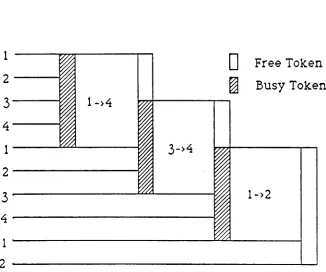
In a token ring (Fig. 2)strategy, access to the transmission channel is con-trolled by passing a permission token around the ring. Any station that wants to transmit should grab this token before putting its nlP~~agpint.o the ring. The sending station is responsible for removing its own message from the ring.

In the type of slotted ring (Fig. 3), a number of fixed-length slots continu-ously circulates around the ring. A full/empty indicator within the slot header is used to signal the state of a slot. Any station ready to transmit should occupy the first empty slot by setting the full/empty indicator to "full" before placing its data into the slot. When the sender receives back the occupied slot, it changes the full/empty indicator to "empty".

(10)

(a) Token ring model

Free Token

Busy

Token

1->2 3->4

1->4 1

2

- - - - 1 , I ' /..."A

3

4

1

2---~lj'/A

3

4

---r'l~/1

1

2

Time

(b) Example of operation

(11)

1 2

3

4

1

2

3

4

1 2

3

4

(a) Slotted ring model

I~

~ ~

r>

v/~ ~,

"/

--

1

i

1

-~

~

~~ ~

~

--

2

2-

2

-~

~

.i

'/

/~

~ j.r/~

~~ I

~~~ I ~ ~~

~

~ ~

\J

~

Time

(b) Example of operation

Fig. 3. Slotted ring control strategy

Closed-loop

model of

empty

slot

empty

g

slot used

L:.J

by

station

(12)

The Order-Access Bus (Fig. S) works as follows: Information transmission occurs in variable-length Frames. A controller provides a start flag at appropri-ate time intervals which signals th~ heginning of a frame. A frame is divided into two parts. a request slot and an arbitrary number of packets. Every sta-tion attached to the bus owns one bit within the request slot. By setting its private bit, a station indicates that it wants to transmit a packet within this frame. At the end of the request cycle, all stations know which of the stations will make use of this frame. The transmission sequence is given by a priority assignment known to all stations.

Under i\LOHA protocol, each user transmits a data packet whenever one is ready. If two or more packets collide (co-exist at the same time), the users involved will realize this after a time period (the collision detection time) and will retransmit their packets after a randomized delay. For details on other related protocols like the SlottedALaR..-\. and Reservation ALOHi\., see [19].

The lJRN protocol is a kind of adaptively controlled Slotted ALOHA pro-tocol. The details are in

[19].

For TDMA and FDMA, the reader is directed to

[26].

(13)

.RandomretranSmissioninterval Station A

Station B

Collision

detection '\

ransmission

I

Aborted

Collision'? .

detection

Fig. 4. CSMA/CD control strategy

Bus sensed busy

-

-.

SuccessfUl transmission

Scheduling

Transmission

(a)Order-access bus model Start Flag

1 2

...

s

...

L

Request slot

I

:&

Frame

, ,

(b) Frame structure

(14)

(conflict) detection and handling mechanism. We also know, on the other hand, that TDMA and FDMA are good control strategies only in the case where all users impose the same amount of traffic.

After comparing the ring type with the bus type topologies, Clark et al. [06] conclude that certain design problems present in a bus do not arise in a ring. Thus it may be somewhat easier to design a ring than a bus. Hence the most appropriate control strategy which complies with hoth our traffic distri-bution and simple control scheme assumptions is the cyclic service scheme.

1.4 Priority Disciplines

From now on, we are going to discuss only ring type topology with token passing (conflict-free) multiple access schemes. In other words, we are going to concentrate on ring type networks with cyclic service scheme only. There have been a number of papers published which 'discussed a single server multi-queue system. Takacs [23] has discussed a M/G/! queueing system with three different orders of service: a) in order, b) random order, and c) reverse order of arrival. In the same paper the distribution functions of the delay and their moments have also been given.

(15)

assuming that the system is stable. Skinner

[21]

concerned with the queueing process on a nonpreemptive priority system with nonzero cross-over time. In that paper the waiting-time distribution function and the queue-size generating function are derived.

Kleinrock

[14]

has compared several multiple access schemes named: Alter-nating Priorities (AP), Round Robin (RR), Random Order (RO), and minislot-ted Alternating Priorities (MSAP) with Polling and Head of Line (HOL) discip-lines. These so-called "New Conflict-Free Multiple Access Schemes", which are simple and effective disciplines in handling customary priority assignment, can be applied to our cyclic service queueing networks.

All these disciplines can be characterized into two categories, namely the Alternating Services and Alternating Priorities. Under the Alternating Services category the server serves only one customer from each queue alternatively, while in the Alternating Priorities environment customers in a queue currently being served have priority over customers in other queues until there are no customers in that queue.

(16)

time) is assumed to be zero. Based on these assumptions, he obtained the equa-tions for the state probability generating funcequa-tions. The approach he used is based on the theorem of complex variables and it is limited to two queues only.

Kuehn

[16]

has also investigated a system similar to the one studied by Eisenberg

[11]

with nonexhaustive cyclic service discipline. The differences are: 1)the number of queues is not limited to two, 2) the switch-over time has been considered. Kuehn provided an approximate analysis of this system. Based on the concept of conditional cycle time and an independence assumption, he obtained the generating function of the stationary probabilities of the state, the Laplace-Stieltjes transform of the delay distribution and waiting time.

The performance analysis of a system using Iflimited" service discipline in

the above mentioned queueing system was reported in Takagi [25]. In a limited service system, a terminal is served until either 1)it is empty, or 2) the number of messages served exceeds a preassigned number during one polling cycle. A polling cycle is defined as the time period between two consecutive polls at the same terminal. For a Poisson arrival process with general distributed service time and non-zero switch-over time, Takagi obtained the mean cycle time and mean message waiting time under the assumption that the traffic among the queues is symmetric (i.e. each queue has the same arrival rate).

(17)

instead of limited. All the papers described above only give the waiting time for the case of symmetric traffic. Kurosawa

[17]

attacked this problem for asym-metric traffic distributions. However, the result turned out to be many complex equations and the exact solution can be obtained only using a numerical approach.

The Alternating Priorities discipline also drew a lot of interest during the past ten to twenty years. Avi-Itzhak et al. [01] initiated the effort in studying a system with exhaustive service discipline. In this discipline, all messages arriv-ing before the server turns idle will be served in the same cycle. After the current terminal finishes service, the server begins to poll the next terminal. The authors formulated the steady-state densities of queueing times, the expected queueing times, and the queueing sizes as well as the first two moments of the busy period based on an MIG/1 queueing model with a switch-over time equal to zero (zero switch rule). Takacs

[24)

also investigated the same model (M/G/l model with two queues) and got the same stationary distribution of the waiting time.

(18)

dis-tributions have been derived.

Cooper and Murray

[08],

and Cooper [09] have solved the same model with two different alternating service disciplines (exhaustive and gated service). In a gated service system. only those messages arriving before the terminal is polled will be served in the current cycle. Other messages arriving after that time will not be served until the next cycle.

Konheim

[1.5]

and Swartz [22] attacked the exhaustive service discipline using different approaches. They extended the works done so far for the two-queue system to a N-two-queue system. Heyman

[12]

studied the exhaustive and gated service disciplines for a high-speed line network called Fasnet and used an approximate approach to solve the mix traffic problem. Only a close-form formula for symmetric traffic has been derived.

(19)

numerical results.

We know without question that this kind of problems is very difficult to deal with. Thus it seems that an approximate analysis approach is necessary. Boxma

[04]

took this step to analyze the limited service discipline. The obtained results compare well with other approximations.

In this thesis, we study the delay performance of the cyclic service scheme with three different disciplines under asymmetric traffic conditions. These three disciplines are: the limited, gated, and exhaustive service disciplines. The sys-tem we analyze can be seen as being somewhere between symmetric and extremely un balanced cyclic queueing systems. In particular, it consists of a number of terminals, one of which is a special terminal and it carries most of the traffic. The remaining traffic is carried by the rest of the terminals, each carrying an equal proportion of the traffic, i.e. the queues in front of the termi-nals are symmetric.

Also, we study the mean cycle time and obtain the probability of an empty queue for the three service disciplines assuming asymmetric arrival rates.

(20)

[18]. In such a system there might be one terminal handling global displaying images for history diagnoses in contrast to other terminals displaying only one branch of these images [02].

In chapter 2, we obtain the mean cycle time for the limited case (k=l). Also, for each of the three service disciplines, we obtain the probability a queue is empty at the instant it is polled. All of the above results are obtained assum-ing that each queue has a different arrival rate (i.e. fully asymmetric arrivals).

In chapter 3, we obtain the mean waiting time in a queue assuming that all the queues have the same arrival rate except a special queue which carries most of the traffic. In particular, we obtain the mean waiting time in a sym-metric queue, in the special queue and in the whole system for each of the three service disciplines.

In chapter 4, we validate the approximate results obtained in chapters 2 and 3 using simulation data.

(21)

2.

MEAN CYCLE TIME AND EMPTY PROBABILITY

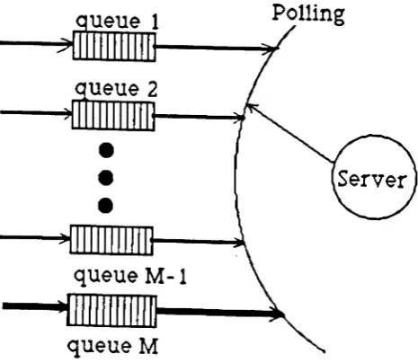
Now we are going to analyze this cyclic service multi-queue system. This system is basically a model of a ring type network with a single channel and a number of terminals. The arrivals at each terminal are assumed to be Poisson distributed. In this chapter, we assume that each queue has a different arrival rate. In chapter 3, we assume that most of the traffic is carried by one particu-lar terminal while the remaining traffic is carried by the rest of the terminals, each carrying an equal amount of the traffic.

The server polls the terminals alternately and serves the customers waiting at that queue according to a prearranged service discipline. Three service dis-ciplines are considered, namely, are the limited, gated, and exhaustive service disciplines. The service time of every customer in each terminal is assumed to be generally distributed with mean b. The server, after finishing serving of a terminal, takes a small non-negative amount of idle time, then polls the next terminal in cyclic order.

(22)

In this chapter, we study the mean cycle time and the probability that a given terminal (queue) is empty at the instant when it is polled by the server for each of the three service disciplines. In the following section we discribe the assumptions under which we analyzed this model. In section 2.2.1 we obtain the mean cycle time and empty probability for the limited service discipline.

In

sections 2.2.2 and 2.2.3 we obtain similar results for the gated and exhaustive service discipline, respectively.

Polling

queue

M

(23)

2.1. Assumptions and Definitions

The assumptions are as follows:

(1) The arrivals at each queue are Poisson distributed, which means that the inter-arrival time at each queue is exponentially distributed with parame-ter Ai (i=1,2, ..,M), where M is the total number of queues.

(2)

The message length of each customer in every queue is generally distri-buted. This means that under a fixed channel capacity (constant service rate) the service time of each customer is generally distributed with the same mean b.

(3) The switch-over time from one queue to the next is also generally distri-buted with the same mean R.

(4)

The arrivals at a particular queue are assumed to be independent of the arrivals at the other queues.

Now let us define some parameters that will be used throughout the

con-text:

M

,\

b

the number of total queues in the system

the arrival rate of the i-th queue

M the total arrival rate of the system (=

L

Ai)

.=1

(24)

b2 : the second moment of the service time of a customer

R: the average switch-over time from one queue to the other

P. : the utilization factor of server i(= Aib )

p : the total utilization of the system (= PI +P2+ · . · +PM)

T_{c :} a random variable indicating the cycle time

C the average cycle time (= ETc)

Co : the average of the cycle time given that no customers are waiting for

ser-vice during a cycle (= MR)

ni: the average number of customers arriving at queue i during one cycle (=

Ii : the number of customers allowed to be served during a cycle.

2.2. Empty probability and mean cycle time

2.2.1 Limited service discipline

From Takagi [25] we know that In a cyclic service multi-queue system under the above assumptions and assuming symmetric arrival rates, the proba-bility that there are no customers in the i-th queue at the instant when it is polled is

Pi 1 - MA(b + R)

(25)

Now we claim that the same probability for the same system but with different arrival rates among the queues is

Pi

M

1 -

2A.

ib - MAjR

1=1

M 1 - ~_~A·b₁

1=1

(i=1,2,... ,M) _(2.2)

This can be shown as follows:

Proof: \\Pe use the notations in Takagi's paper. Let

F.(Zl,Z21 ... ,ZM): the z-transform of the joint P~IF of the number of messages

at each station i (i=1,2, ...,M) at the instant when the i-th station is polled

Ai(z):

B(z):

R(z):

the z-transform of the probability mass function (PMF') of the arrival process of the j-th queue

the z-transform of the PMF of the service process the z-transform of the PMF of the switch-over process

According to Takagi [25], the z-transform of the joint PMFof the number of messages at each queue at the instant when the current queue is polled can be expressed by the z-transform of the joint PMF at the instant when the pre-vious queue is polled . The relationship between these two z-transforms is as

(26)

_0_ Fi,1(1,1, ... ,1) = AjR + Ajb [1-Fj(1,..,1,O,1,..,1)]

OZj

- [1-

F_J(1,..,1,0,1, ..,1)] - _0_

r,

(1,1~

... ,1) for j =i

dZj

_0_ F_{i • 1}(1,1,...,1) = AJR + Ajb [1-Fj(1,..,1,O,1,..,1)]

OZj

+ _0_ F_i(1,1,... ,1) for j~i (j=I,2, ...,Af)

OZj

After sum up these M equations, for each j (j=1,2, ...

,M)

we have:

1 - Fj(1,..,1,0,1, ..,1)

=

M~jR

+

~jb~

[1-Fi(1,..,1,O,1, ..,1)] 1=1

Then we sum up these equations for all j (j=1,2, ...,M), we get

~

[1-Fi(1,.. ,1,O,1,..,1)] 1=1

hence

(2.3)

(2.4a)

(2.4b)

(2.5)

(27)

f

[1-Fi(1... ,1,O,1,..,1)

I

1=1 1 - p

(2.7)

The equation above can be interpreted as the average number of customers served in one cycle (LHS)equals the average total number of arrivals during one cycle (RHS). It is known that Fj (1,..,1,0,1, ..,1) is the probability that the j-th

queue is empty when polled. From Eq.(2.5) and (2.7)we get:

1 - Fj (1,.. ,1,O,l, .. ,1)

= M'AjR + Ajb _M

1 - ~_.-:.-A·b_J

i=l

M'AjR

1 - p (2.8)

Hence the probability that the j-th queue is empty at the instant when it is polled can be expressed as follows:

Pi = Fj (1,.. ,1,O,1,.. ,1)

M

l - ~ A · b - M A · R_~ I J

i=l

M

1 -

v

_~

x.»

₁

i=1

1 - P - M'AiR

1 - p

(28)

M

C = MR + b

L

[1 - Fi(l".. ,l,O,l, .. ,l)!

i=l

we can derive the average cycle time for the limited service discipline with no more than one customer served per poll (Ii =

1).

The average cycle time is

c = AiR ~\JR

1 - p

(2.9)

2.2.2. Gated service discipline

From lemma 3.2 in Rubin [20) we know that in steady state, the mean cycle

1 - P

MIl M 1 - ~p_~ _I

.=1

time of the gated service discipline equals to c =

-For the gated and exhaustive type service disciplines under the assumption of independence, it is also true that we can obtain the probability that a given queue is empty at the instant when it is polled. In a gated service discipline, the probability that the j-th queue is empty means that there are no customers arrived at the j-th queue for exactly one full cycle.

(29)

But according to the phenomenon of "length-biased sampling" in renewal process, this probability is a little higher which can be approximated as

p,. = e - ,\Je ( 1 - P, ) ( ._{) = ,_,...}14)

,.Y.

, .{ )

(2.10) 2.2.3. Exhaustive service discipline

From lemma 4.2 in Rubin

[201

we know that in steady state, the mean cycle

1 - p Co

=

-»n

AI

1 - ~Pi

i=l

time of the exhaustive service discipline equals to e = - -_ _

Now let us look into a "cycle". First, it is legitimate to subdivide each cycle into At pairs of time periods. Each pair (R"S,)reflects the time it takes for the server to switch from the i-th queue to the (i+l)st queue (R,),and the time it takes for the server to serve the customers in the current queue (s.), This is shown in Fig. i .

Fig. 7 The sub-divisions of a cycle

L

emma 2 1 ·. . In steadv state if both the gated and the exhaustive service dis-J '

(30)

the time period required by the server to serve queue i (s;)for these two discip-lines are the same.

Proof: Based on that the gated and the exhaustive service disciplines have the same average cycle time and the independence assumption that the arrivals at each queue is independent of the arrivals of other queues, the average number of arrivals per cycle at the corresponding queues for these two service discip-lines will have the same limit. Which means that in the gated discipline, the average time that the server spends on serving the customers of the correspond-ing queue equals to the average time the server spends on servcorrespond-ing the customers of the exhaustive service discipline. This is to say that the corresponding queues in both service disciplines will have the same average length of Si.

Lemma 2.2: For the gated and exhaustive service disciplines, the average time that the server spends on serving the customers in the i-th queue is

g-; = lv/ Pi R

• 1 - P (2.11 )

Proof: In order to prove this lemma, we use some notations which used In

Rubin [20] for the gated service discipline and listed as follows:

Vi(k1 , • • • ,kM ) = The steady state probability that kj messages at queue J

(31)

x

~ Z k, • • • z lewv (Ie ••• Ie ) ~ 1 M i l ' , M

lcu=O

It can be shown that

(2.12)

M

where 11 =

II

Ai(Zi) and B,(1')) appears In the i-th component of the vector

i=1

Z = (Zl, · • • ,ZM). Now let us define:

v(i,j) = -d-Vi(l,...,l)

dZj

Then v(i,j) is the number of customers at the j-th queue at the instant that the server is available to the i-th queue. So v{i+l,i) is the total number of arrivals at the i-th queue during the period from the the beginning of serving the i-th queue to the beginning of serving the (i+ 1)st queue. In other words, v{i

+

1

,i)

is the average number of arrivals during the time period (Si + Ri ) . So

Then we can find out the following equation (indexes i, j, and k are modular M):

i-I

v(i,i)

=

x,

L(S"; + R;) for i

>:

(32)

[

M i - I

I

v(i,j) =

x,

2:

(3'; + R;) +

2

(3'; +

1fJ

for i~j

k=i k=l

(2.13)

From this we know that v(i,i) is the average number of arrivals at the i-th

queue for a whole cycle. Based on this knowledge, we will have the following

equation:

(2.14 )

A·

which has the same meaning as v(i,i)

=

.u: v(i,i) (1 ::f £,) -s .\1). Now we are

Ai

going to find out v(i,j) for each i and j

(1

:s i,j ~ At). From the definition of

v(i.i)we can derive

v(i+1,j} = AiR..,. v(i,j) + p,v(i,i} for i=l=j

v(i+1,i) = AiR + Piv(i,i) Cor i=j (2.15)

After summing up those equations for all the different i

(1

-s i :sM) we will get

M M M

L v(i,j) = MAi R +

2

v(i,i) - v(i,i) + Pi L v(i,i)

i=l i=1 i=l

M M

= MA,R +

2

v(i,j) - v(j,j) + Pi

L

~

v(j,j)

1=1 i=l Pi

M M

= MAiR + Lv(i,j) - v(i,i) + v(j,j)2:Pi

i=1 i=1

(2.16)

From the above equation we can get v(j,j) = MAjR + v(i,i)p. Which

MA·R

means that v(j,j) = ' . Thus it is true that

(33)

v(M,M) AM

AIR

=

-1 - P

From Eq.(2.13), we can find out without difficulty that

v(i+l.1) - ~ =

g;

+ R.

Ai Ai

From Eq.(2.16) it can also be shown that the left part of the above

equa-· 1 R [ MPi

1

Mp,

tion equa s to 1 + - - .So we can get

s-:

= R--'-.

1 - P 1 - P

Lemma 2.9: The probability that the j-th queue has no customers waiting for service at the instant it is polled is

-~ ~(l-v·)

Pi = e ' ,

Proof: For an exhaustive service discipline, at the instant when the server leaving a queue, there will be no customers waiting in that queue. Hence, from the time when the server finished service of the j-th queue to the time when the j-th queue is polled the next time is e - Sj. We know the arrival of each queue is a Poisson process, so the probability that no customer arrived during that

But due to the same length-biased sampling problem, this probability will be a little higher which can be approximated as follows:

-A.~(1-V)2

(34)

3.

THE MEAN WAITING TIME (APPROXIMATE ANALYSIS)

3.1. Some results from Takagi's and Rubin's papers

In Rubin [20] and Takagi [25], we find exact results of the average waiting time for the cases of balanced (all the queues have the same arrival rate) and extremely unbalanced traffic (all the traffic goes through only one of the queues) for the three service disciplines under study . l~.\ modifying the equa-tions of the mean waiting time which given in these two papers, we obtain all approximation for the average waiting time in the system, the average waiting time in the special queue, and the average waiting time in the symmetric queues for each of the three disciplines. These approximate expressions are more complicated than their counterparts in the symmetric or the extremely unbalanced cases. The following equations give the average waiting time for the symmetric case:

WL 1 [M'Ab2 He 2 (l+'Ab)MR

="2

l-MA(b+H) + R + l-MA.(b-Hj

WG =

1.-

[MA.b2

.... He 2 + (1+A.b)MH

1

2 I-M'Ab R I-MAb

WE =

.!.

[MAb2 _-- _He ₂ ₊ _(l-'Ab)MR

1

2 I-MAb R I-MAb

where:

M'AR2

c

2

1

+ R

I-MA(b+R)

(3.1)

(3.2)

(35)

WL

=

average waiting time of limited service system

WG

=

average waiting time of gated service system

WE

=

average waiting time of exhaustive service system

A= mean arrival rate of each queue

b

=

average service time of each message

b2 = second moment of service process

R

=

mean switch-over time from one queue to the next

M

=

total number of terminals

The following equations give the average waiting time for the extremely unbal-anced case:

w

L

z

WG_2;

WE z

where:

(3.4)

(3.5)

(3.6)

W%L

=

average waiting time of limited service system

(36)

s;

=

mean arrival rate of the special queue

bx

=

average service time of each message

bx,2

=

second moment of service process

For the convenience of later discussion, let us define some parameters which are

used throughout this chapter. Define:

1.)The total arrival rate of the system:

.\1

;'\ ~A,

i=l

2.) The traffic distribution coefficient:

0.,

MAo

- - '

.\

3.) The weighted traffic distribution coefficient:

~~

~ <Xi

j=1 A

4.)The factor of symmetry:

M-(3

"Y =

M-l

(37)

M M 2 1 '2

L

A_i2

"" A. .

~ ,

= i=l i=l

eTA

M M

6.) The equivalent mean arrival rate of a queue in the system:

.\ ,\

~ = - + <T

Af "

3.2. Limited Service Discipline

3.2.1 Average Waiting Time in the Special Queue

From the simulation result, it is easy to find that thp average waiting time

In the special queue is somewhere 'between' that of the symmetric and the extremely unbalanced cases. We note that, in the denominator of equations (3.1) and (3.4), there are different coefficients in front of the average switch-over time ("1" in Eq.3.1 and"M" in Eq.3.4) corresponding to different traffic conditions. If we let these two figures (nI" and ".\1n) to be the traffic distribu-tion coefficients of the symmetric and extremely unbalanced cases, a j might be

one possible way to define this coefficient. The coefficient defined here equals the arrival rate of the special queue divided by the average arrival rate of each queue in the system. Another modification for all the equations hereafter is that

M

we replace the factor nMAn by "~

x, ".

This modification is due to the change in

i=l

(38)

M

~A.b~ 1 , - I

2 M

1-~A,(b+OMR)

, - I

(l-t-"Mb)MR

ft"t

1-~X,(b+ct.wR )

• - I

M

1 - ~A,(b+fIMR) , I

(3.7)

3.2.2 Average Waiting Time in other Queues

Almost the same approach we did for the special queue can be applied to evaluate the waiting times in the other queues. Now we replace aM and "-.\1 in

Eq.3.7 with 01 and AI n--pectively. V'le also multiply the third term in Eq.3.7

with a term "'Y to account for the change of the traffic distributions. Since the

third term of Eq.3.7 is mainly a term concerning about the switch-over time, as the traffic of the symmetric queues decreases this term will not contribute to the waiting time very much. On the other hand, this term would be an impor-tant factor when the traffic is evenly distributed among the queues of the sys-tern. The parameter 'Y could reflect these variations. The average waiting time

in the symmetric queues can be approximated as

W,L

J

M

L

A,b~ 1 ,-I

2 M

1-~Ai(b+oIR)

, - I

(1+AJb)MR

M

1-~A,(b+uIR)

• - I

MAJR~CR~

M

1-_~A.(b+uIR)

.-1

(3.8)

(j = 1 - M-1)

(39)

If we consider the average waiting time in the system (the average waiting time of all the customers in the system), a system with traffic evenly distributed among the queues has the minimum average waiting time. As a matter of fact, with the total arrival rate fixed, the average waiting rirue in the system will become larger as the variance of the"M" arrival rates goes higher. Let the vari-ance of the"

u»

individual arrival rates be the measun- of the degree of asym-metry of the traffic condition in this system. Vv~e then get the knowledge that the mean waiting time of the system will increase when the degree of asym-metry increases. One way to reflect this phenomenon is by using a parameter named equivalent mean traffic (~) to account for the variation of the degree of asymmetry.

In the denominator of equations 3.7 and 3.8 we employ different traffic dis-tribution coefficient as the coefficient of

"R"

in evaluating the mean waiting time in the corresponding queue. To find the mean waiting time in system, by considering that the waiting time as the weighted waiting time among all the queues in the system, we use the weighted traffic distribution coefficient n13n

instead of n1" and nM" in the equations stated above respectively. The approxi-mate equation of the mean waiting time in the system is

M

~A,b2

(40)

3.3. Gated Service Discipline

3.3.1. Average Waiting Time in Special Queue

We use the same assumption as in the previous section (sec.3.2) namely

that the average waiting time in this special queue is somewhere between those

of the symmetric and the extremely unbalanced cases. When the arrival rate of

this special queue is almost the same as the arrival rate of each of the

sym-metric queues, the average waiting time of the special queue will close to the

waiting time of each queue in a fully symmetric system. On the contrary, as the

arrival rate of the special queue gets larger, the average waiting time of the

spe-cial queue will close to the average waiting time of the spespe-cial queue in an

extremely unbalanced system. This is to say that the average waiting time of

these two cases are the lower and upper bounds of the average waiting time of

the special queue in this system. Hence we can get the approximate average

waiting time by simply weighting the waiting times of these two bounds (Eq 3.2

and 3.5). The weighting factors with respect to the average waiting times of the

MA-the symmetric and MA-the extremely unbalanced cases are 1 - M and

(M-l)/\

MAM

The approximate average waiting time In the special queue thus

(M-l)!\ .

(41)

W_.WG ~"[x,,w

(JI -1)/\

M'A.M

(M -1):\ W",G (3.10)

3.3.2. Average Waiting Time in other Queues

By noting the phenomenon that when the arrival rate of the special queue increases, the decrement of the average waiting time in the other queues is not in proportion to the increment of the arrival rate of the symmetric queues. So it is not enough for us to reflect this change by simply replacing the arrival rate 'A.

in the nominator of the third term of equation 3.2 with 'Aj . Hence we

approxi-mate this average waiting time by multiplying the last term in equation 3.2 .w

2,PJ-P,

with 1 -t- 2 i=l to account for different variations of traffic combination.

iW-1

Here Pic

=

A.Ieb is the utilization factor of the k-th queue as defined in chapter 2.

The modified equation is as follows:

(3.11 )

M

1

~p.-p.

~ 1 , (l+-'A.:Mb)MH

1 + 21=1

--~--J'J-1

1-~Aib

i=l

.W

, x'·b₂

~ ,

i=l

- - - - + RCR2 +

1

=

-2 W·G

1

( j = l - M - l )

(42)

"Ve change one parameter in the third term of equation 3.2 by the same reason we did in section 3.2.3. to get the approximate equation for the average waiting time in the system. The changing parameter is ~ which, instead of the changed parameter A., could reflect the actual equivalent mean arrival rate of

the system in evaluating the average waiting time in the system. Thus the approximate average waiting time in the system is

1 2

i=,W

~ Aib2 i=l

,W

1 - " A·b~ I

i=1

(3.12)

3.4. Exhaustive Service Discipline

3.4.1. Average Waiting Time in Special Queue

The modification in this system is almost the same as that in the gated ser-vice system. We can approximate the average waiting time in the special queue exactly the same as that in the gated system except that the average waiting in the special queue should weight between that of the symmetric and the extremely unbalanced cases of the exhaustive service discipline. Hence the approximate average waiting time in the special queue is sp

( JfA.M

1

MX.

W E = 1 - WE +. M E

(43)

3.4.2. Average Waiting Time in other Queues

The same reasoning in section 3.3.2 can be applied to find the average waiting time in the symmetric queues except some of the sign changes. By not-ing the phenomenon that when the arrival rate of the special queue increases, the increment of the average waiting time in the other queues is not in propor-tion to the decrement of the arrival rate of the symmetric queues. So it is not enough for us to reflect this change by simply replacing the arrival rate 'A in the nominator of the third term of equation 3.3 with 'Aj . Hence we approximate this

average waiting time by multiplying the last term in equation 3.3 with M

'p.-p._~ ₁ _,

1 - 21=1 to account for different variations of traffic combination. The

M-1

modified equation is as follows:

W·E

]

1

2 M

1-~_~A·b

.

1= 1

[

~

p.-p ~ J '

_ He 2 + 1 - 2_i=_1 _ _

R M-l

(i 1 - M-1)

,'vi

l-''A·b~

.

1=1

(3.14)

3.4.3. Average Waiting Time in System

(44)

changed parameter A, could reflect the actual equivalent mean arrival rate of

the system in evaluating the average waiting time in the system. Thus the

approximate average waiting time in the system is

1

2 M

l-~A·b~ ,

i=l

(l-~b)MR

.... HCR 2 + -

M-1-~_~A·b_s

i=l

(45)

4. VALIDATION - NUMERICAL EXAMPLES

The approximate results obtained in chapters 2 and 3, were validated by comparing them against simulation data. The simulation model was developed to simulate a number of terminals served by the same cyclic server. The simula-tion model was run assuming four terminals. It was also run assuming eight ter-minals. The special terminal carries extremely high traffic while the others are symmetric terminals. We simulated the system assuming that the sum of all the arrival rates to all the terminals is equal to 0.6 messages/second. This was allowed to increase to 1.0 and 1.4 messages/second. For each of these values, the individual arrival rate to each symmetric queue and the special queue were varied. All inter-arrival times were assumed to be Poisson distributed. The message length was assumed to be exponentially distributed with mean equal to 4,000 bits. The channel capacity was as~urned to be fixed at 8,000 bps. The time it takes the server to walk between each pair of neighboring terminals was assumed to be exponentially distributed with mean equal to 100 ms. We also simulated the system assuming a mean switch-over time equal to 50 ms.

(46)

Pro-350 machine under the \~NIXoperating system environment using C. In the following tables (table (4.1)to (4.33))we list simulation and approx-imation results for

a) the mean waiting time in a symmetric queue,

b) the mean waiting time in the special queue,

c) the overall mean waiting time,

d) the probability that the symmetric queue isempty, and

e) the probability that the special queue is empty.

We also present the error ratio for the different cases simulated. The error ratio shown is computed as follows:

(47)

4.1 Limited Service discipline

The results are given in tables 4.1 to --1.9. The mean service time is equal to 500 ms, The system is assumed to consist of four terminals (tables 4.1 to 4.5) or eight terminals (tables 4.6 to 4.9). The switch-over time was set to 50 ms or 100 ms.

Table 4.1: M=4, mean switch-over time = 100 InS

sum of the arrival rates

=

0.6 msg/sec.

Al 3 A4 item simulation approximation error%

0.06 0.42 WI 3L 513.09 468.70 -8.65

PI 3L 0.9663 0.9657 -0.06

W.L 827.60 802.63 -3.02

P4L 0.7602 0.7600 -0.03

w

L _734.36 _722.30 _-1.64

0.10 0.30 Wi 3L 573.27 563.13 -1.77

PI 3L 0.9426 0.9429 0.03

W 4L 748.09 715.52 -4.35

P4L 0.8277 0.8286 0.11

(48)

Table 4.2: M=4. mean switch-over time

=

100 ms sum of the arrival rates = 1.0 msg/sec.

item simulation approximation error%

0.167 0.50 WI 3L 993.93 1079.07 8.57

Pi 3L 0.8668 0.8667 -0.01

W..L 1966.83 1749.97 -11.02

P..L 0.5997 0.6000 0.05

WL _1480.79 _1406.32 _-5.03

Table 4.3:M=4, mean switch-over time

=

100IDS

=

1.4 msg/sec.

Al 3 A₄ item simulation approximation error%

0.30 0.50 WI aL 2561.16 3279.49 28.05

0.6199 6310.34

0.3697 3895.92

0.6000 6150.00

0.3333 4028.06

(49)

Table 4.4: M=4, mean switch-over time

=

50IDS

sum of the arrival rates = 0.6 msg/sec.

0.10 0.30 Wt 3L 380.68 383.,58 0.77

Pi 3L 0.9714 0.9714 0.00

w

L

457.69 441 .• , _-3.53

4

P.L 0.9147 0.9143 -0.04

WL _419.07 _423.,)0 _1.06

Table 4.5: M=4, mean switch-over time = 50 ms sum of the arrival rates

=

1.0 msg/sec.

0.167 0.50 W. 3L 678.46 768.85 13.32

PI 3L 0.9333 0.9333 0.00

W4L 1069.68 968.74 -9.43

p.L 0.8014 0.8000 -0.17

(50)

=

~l 7 item simulation approximation error%

0.06 0.18 WI 7L 896.41 890.37 -0.67

PI 7L 0.9317 0.9314 -0.03

WsL 1165.26 1116.91 -4.15

PaL 0.7937 0.7943 -0.08

WL _977.47 _976.71 _-0.08

=

100 ms sum of the arrival rates = 1.0 msg/ser.

0.10 0.30 WI 7L 1535.74 1614.76 5.15

PI 7L 0.8403 0.8400 -0.04

WsL 3261.89 2826.92 -13.34

PaL 0.5192 0.5200 0.15

(51)

Table 4.8: M==8, mean switch-over time

=

50 ms sum of the arrival rates = 0.6 rnsg/sec.

0.06 0.18 WI 7L .)39.88 540.33 0.08

PI 7L 0.9656 0.9657 0.01

WaL 626.86 613.8·5 -2.07

PaL 0.8971 0.8971 0.00

WL _565.95 573.09 -0.39

=

50 rns sum of the arrival rates = 1.0 msg/sec.

0.10 0.30 WI 7L 957.61 1008.91 5.36

PI 7L 0.9200 0.9200 0.00

WaL 1473.34 1296.05 -12.03

PaL 0.7604 0.7600 -0.05

(52)

4.2. Gated Service Discipline

The results are given in tables 4.10 to 4.21. The mean service time is equal

to 500 ms. The system is assumed to consist of four terminals (tables 4.10 to

4.15) or eight terminals (tables 4.16 to 4.21). The switch-over time was set to 50 ms or 100 ms.

Table 4.10: M=4, mean switch-over time = 100 ms sum of the arrival rates == 0.6 msg/sec.

A.1 3 A.4 item simulation approximation error%

0.06 0.42 Wi 3G 544.56 523.26 -3.91

PI 3G 0.9668 0.9673 0.05 w

..

G _626.50 _631.43 _0.79

P.G 0.8005 0.8273 3.35

WG _602.05 _593.70 _-1.40

0.10 0.30 WI 3G 558.33 544.29 -2.51

PI 3G 0.9458 0.9472 0.15

W..G 599.67 614.24 2.43

P.G 0.8514 0.8644 1.53

(53)

=

1.0 msgfsec.

At 3 A4 item simulation approximation error%

0.10 0.70 ",' 1 3G 881.34 886.00 0..53

PI 3c. 0.9269 0.9268 -0.01

\.{' G

..

_1115.54 _1140.00 _2.19

P4G 0.6949 0.6389 -8.06

WG _1045.47 _1051.96 _-0.62

0.167 0.50 WI 3G 946.76 935.19 -1.22

PI 3G 0.8815 08850 0.40

W4G 1085.29 1100.00 1.36

P4G 0.7108 0.7408 4.22

(54)

=

lOO ms sum of the arrival rates

=

1.4 msg/sec.

A.1 3 A.4 item simulation approximation error%

0.20 0.80 WI 3G 1742.71 1803.33 3.48

PI 3G 0.7989 0.7866 -1.54

W.G 2175.23 2266.67 4.20

P4G 0.5042 0.5273 4.58

w

G _1989.75 _2086.60 _4.87

0.233 0.70 WI 3G 1837.52 1845.30 0.42

PI 3G 0.7723 0.7597 -1.63

W.G 2224.47 2233.34 0.40

P.G 0.5374 0.5452 1.45

(55)

=

50 ms sum of the arrival rates

==

0.6 msg/sec.

0.10 0.30

w,

3G 380.07 379.29 -0.21

PI 3G 0.9724 0.9732 0.08

W4G 406.66 414.29 1.x~

P.G 0.9217 0.9297 0.87

WG _393.36 _399.04 _1.43

(56)

-Table 4.14: M=4, mean switch-over time

=

1.0 msg/sec.

Ai 3 "-4 item simulation approximation error%

0.15 0.55 Wt 3G 713.66 711.33 -0.33

Pl 3G 0.9458 0.9460 0.02

W.G 812.43 805.00 -0.91

P.G 0.8309 0.8526 2.61

wG _768.19 _767.32 _-0.11

0.167 0.50 WI 3G 699.89 717.59 2.53

Pl 3G 0.9396 0.9407 0.12

w G _799.34 _800.00

0.08

4

P4G 0.8437 0.8607 2.01

w

G _749.66 _764.43

(57)

Table 4.15: ~1=4, mean switch-over time

=

50IDS

sumof the arrival rates

=

1.4 msg/sec.

Al 3 _A" item simulation approximation error%

0.20 0.80 Wi 3G 1403.50 1485.00 5.81

Pi 3G 0.7989 0.7866 -1.54

wG

4 _1747.77 1716.67 -1.78

P4G 0.5042 0.5273 4}58

WG _1599.56 _1626.63 1.69

0.233 0.70 WI 3G 1837.52 1845.30 0.42

PI 3G 0.8782 0.8716 -0.75

W"G 2224.47 2233.34 0.40

p"G 0.7318 0.7384 0.90

(58)

=

0.6 msg/sec.

0.03 0.39 WI 7G 816.47 814.46 -0.25

PI 7G 0.9664 0.9668 0.04

W₈G 957.97 968.57 1.11

PsG 0.6613 0.6985 5.63

w

G _908.37 _891.16 _-1.86

--

-0.06 0.18 WI 7G 854.08 842.77 -1.32

PI 7G 0.9344 0.9357 0.]-t

WsG _894.17 _908.57 _1.61

PsG _0.8195 _0.8~93 _1.20

w

G _866.16 _868.48

(59)

=

100 ms

=

1.0 msg/sec.

A.8 item simulation approximation error%

0.10 0.30 WI 7G 1370.67 1366.00 -0.34

PI 7G 0.8592 0.8590 -0.02

wsG 1487.88 1520.00 -0.10

PsG 0.6555 0.6650 1.4.5

(60)

=

1.4msg/sec.

Al 7 As item simulation approxirnat ion error%

0.10 0.70 Wi 7G 2482.90 2496.67 -0.55

PI 7G 0.7834 0.7762 -0.92

WsG 3201.70 3133.33 -2.14

PsG 0.2930 0.2972 1.43

WG _2842.31 _2798.95 _-1.53

0.14 0.42 WI 7G 2567.88 2586.27 0.73

PI 7G 0.7196 0.7067 -1.79

WsG 2903.59 2946.67 1.48

PsG 0.4382 0.4128 -5.80

w

G _2668.23 _2728.40

(61)

=

0.6 msg/sec.

Al 7 As item simulation approximation error%

0.05 0.25 WI 7G 504.08 523.78 3.91

Pi 7G 0.9724 0.9725 0.01

w,

G 563.11 571.43 1.48

PsG 0.8727 0.8825 1.12

WG _528.83 _545.16 _3.09

0.06 0.18 WI 7G 528.36 528.53 0.03

PI 7G 0.9668 0.9673 0.05

WaG 560.47 561.43 0.17

PsG 0.9068 0.9106 0.42

(62)

=

0.10 0.30

WI 7G 925.18 935.19 0.85

0.9261 1014.90

0.8079 952.02

0.9268 1010.00

0.8155 963.23

(63)

=

1.4 msgjsec.

At 7 As item simulation approximation error%

0.10 0.70 Wi 7G 1690.91 1831.67 8.32

PI 7G 0.8853 0.8810 -0.49

WsG 2136.21 2150.00 0.65

PsG 0.5369 0.5452 1.55

w

G _1913.32 _1982.81 _3.63

0.14 0.42 WI 7G 1901.08 1876.47 -1.29

PI 7G 0.8475 0.8406 -0.81

WsG 2157.38 2056.67 -4.67

PsG 0.6596 0.6425 -2.59

(64)

4.3. Exhaustive Service Discipline

The results are given in tables 4.22 to 4.33. The mean service time is equal to 500 ms. The system is assumed to consist of four terminals (tables 4.22 to 4.27) or eight terminals (tables 4.28 to 4.33). The switch-over time was set to 50 ms or 100 ms.

=

0.6 msg/sec.

Al 3 Aet item simulation approximation error%

0.06 0.42 WI 3E 562.43 574.69 2.18

PI 3E 0.9676 0.9683 0.07

WetE 471.80 468.57 -0.68

petE 0.8337 0.8609 3.26

WE _499.00 _506.30 _1.46

0.10 0.30 WI 3E 541.44 553.81 2.28

PI 3E 0.9481 0.9497 0.17

W.E 493.25 485.71 -1.53

petE 0.8702 0.8835 1.53

(65)

=

100fiS

=

1.0 msg/sec.

Ai 3 A. item simulation approximation error%

0.10 0.70 Wi 3E 1101.14 1006.00 -8.64

Pt 3E 0.9322 0.9303 -0.20

W4E 733.36 760.00 3.63

P.E 0.7237 0.7893 9.06

WE _844.16 848.04 0.46

0.167 0.50 Wi 3E 980.16 957.41 -2.32

Pi 3E 0.8928 0.8940 0.13

W.E 795.45 800.00 0.57

P.E 0.7666 0.7985 4.16

(66)

Table 4.24: rvf=4, mean switch-over time

=

1.4 msg/sec.

0.20 0.80 WI 3E 1985.04 1936.67 -2.44

Pi 3E 0.8245 0.8057 -2.28

W

4E 1358.71 1.500.00 10.40

P.E 0.6207 0.6811 9.73

WE _1628.67 _1680.06 _3.15

0.233 0.70 Wi 3E 2097.16 1897.16 -9.54

PI 3E 0.8034 0.7845 -2.35

W₄E _1499.11 _1533.33 _2.28

P4E 0.6380 0.6741 5.66

(67)

Table 4.25: M=4, mean switch-overtime

=

50 rns

=

0.6 msg/sec.

0.10 0.30 WI 3E 376.72 384.05 1.95

Pi 3E 0.9739 0.9745 0.06

W.E _339.91 350.00 2.97

p.E 0.9325 0.9400 0.80

(68)

=

1.0 msg/sec.

At 3 A. item simulation approximation error%

0.15 0.55 WI 3E 805.73 734.67 -8.82

PI 3E 0.9498 0.9500 0.02

~V-lE 606.18 645.00 6.40

p.E 0.8669 _0.8908 2.i6

WE _695.80 _682.68 _-1.89

0.167 0.50 WI 3E 757.80 728.70 -3.84

PI 3E 0.9449 0.9455 0.06

W.E 598.06 650.00 8.68

p.E 0.8731 _0.8936 _2.35

(69)

Table 4.27: M=4, mean switch-over time = ,50 ms sum of the arrival rates = 1.4 msg/sec.

0.20 0.80 WI 3E 1710.33 1551.67 -9.28

Pi 3E 0.9062 0.8976 -0.95

W.E 1133.91 1333.33 17.59

P.E 0.7852 0.8253 4.97

WE _1382.18 1423.37 2.98

0.233 0.70 WI 3E 1675.84 1531.92 -8.59

PI 3E 0.8857 0.8951 1.06

WE

..

1195.39 1350.00 12.93

P4E 0.7951 0.8211 3.27

(70)

=

100IDS

==

0.6 msg/sec.

0.03 0.39 WI 7E 864.33 856.09 -0.95

PI 7E 0.9668 0.96i3 0.05

l{'''sE _699.75 _702.86 _0.44

PsE 0.7072 0.7491 5.92

WE _757.37 _780.27 _3.02

0.06 0.18 WI 7E 827.70 828.07 0.04

PI 7E 0.9367 0.9375 0.09

WsE 774.07 762.86 -1.45

P8E 0.8330 0.8434 1.25

(71)

Table 4.29: ~1=4, mean switch-over time = 100 ms

=

1.0 msg/sec.

r

-item simulation approximation error%

0.10 0.30 WI 7E 1321.61 1331.71 0.76

Pi 7E 0.8652 0.8655 0.03

~V8E 1181.61 1180.00 -O.lt

PsE 0.6910 0.7069 2.:~O

WE 1279.54 1273.54 -0.47

=

1.4 msg/sec.

0.14 0.42 Wi 7E 2514.52 2586.27 -1.39

Pi 7E 0.7379 0.7240 -1.88

WsE 2164.62 2153.33 -O.5~

PsE 0.5059 0.4971 -1.74

(72)

=

0.6 msg/sec.

0.05 0.25 WI 7E 536.29 525.84 -1.95

PI 7E 0.9726 0.9732 0.06

WeE 480.60 478.57 -0.42

PeE 0.8873 0.8964 1.03

WE _513.33 _504.84 _-1.65

0.06 0.18 WI 7E 519.93 521.18 0.24

PI 7E 0.9677 0.9683 0.06

WsE 488.71 _488.57 _-0.03

PsE _0.9131 _0.9184 _0.58

(73)

=

1.0 msg/sec.

0.10 0.30 WI 7E 933.18 915.86 -1.86

Pi 7E 0.9296 0.9303 0.08

~'sE 836.34 840.00 0.44

PsE 0.8303 0.8408 1.26

WE _904.12 _886.77 -1.92

=

1.4 msg/sec.

itern simulation approximation error%

0.14 0.42 Wi 7E 1868.33 1836.47 -1.71

PI 7E 0.8604 0.8509 -1.10

WaE 1569.49 1660.00 5.77

PaE 0.7102 0.7050 -0.73

(74)

In the case of low traffic [i.e. the sum of all the arrival rates equals 0.6 message/second), the error percentage of the approximate mean waiting time is within one or two percent. It seldom exceeds five percent when the sum of the arrival rates is equal to 1.0 msg/sec. In the case of high traffic [i.e, the sum of all the arrival rates equals to 1.4 msg/sec), the error percentage increases to around ten percent for the gated and the exhaustive service disciplines. It goes even higher for the limited service discipline. Thus, we have a good approxima-tion for the gated and exhaustive service disciplines. For the limited service discipline, the approximation is reasonable when comparing with Boxma's results

[04].

(75)

5. CONCLUSION AND SUGGESTION

In this thesis, we have discussed a cyclic service multi-queue system with asymmetric arrival rates to the queues of the system. \\ie concentrated on a specific pattern of arrival rates. In particular, one of the terminals carried most of the traffic. The remaining traffic was carried by the rest of the terminals, each carrying an equal proportion of the traffic. This type of queueing model can be used to study different ring type of local area networks.

This model was analyzed under three different service disciplines, namely, the limited, the gated, and the exhaustive service disciplines. The analysis of this model involved: a) the derivation of the exact expression for the mean cycle time for the limited service discipline (K=1); b) the exact expression for the empty probability for the limited service discipline: c) an approximate expres-sion for the empty probability for the gated and the exhaustive service discip-lines; d) an approximate expression for the mean waiting time in the special queue, in one of the symmetric queues, and in the whole system for each service discipline.

(76)

partie-ular, we obtained an approximate solution for the average waiting time in each of the queues and in the system. We compared the approximate results with results from simulation for a number of traffic combinations ranging from low utilization (0.6 messages/second) to high utilization (1.-1 messages/second).

The approximate result for the average waiting time in each queue and in the system for the gated and the exhaustive service disciplines turned out to be very good when compared with the simulation data. Most of the time the error percentage was within a few points. It seldom exceeded ten percent for almost all the cases. The approximate results for the average waiting time in each queue and in the system for the limited service discipline compare favorably with other approximate results such as those obtained hy Kuehn and Boxma which listed in Boxma

[04].

In particular, the error percentage is better than Kuehn's. It is a little higher than that of Boxma's in low utilization traffic, but

it is at the same level for high utilizations.

(77)

to calculate the approximate probability that there are no customers in a queue when it is polled. This provides some information which might be useful in net-work design.

Although in this thesis we merely considered the case where only one ter-minal is different from the others, this might farilit ate us to investigate other similar systems. Several extensions can be considered, For example: 1) the arrival rates are all different (a totally asyrnrnet.ric syste-m], 2) the service time of each queue has a general distribution with different mean, and 3) the same limited service system but with different preassigned numbers (2, or 3, etc. instead of 1 considered in this thesis).

(78)

REFERENCES

[01] B. Avi-Itzhak, W. L. Maxwell, and L. W. Miller, "Queuing with Alternat-ing Priorities," Operations Research 13 (1965).

[02] B. S. Baxter and M. P. Zeleznik, "Communication and Storage Protocols for PACS," IEEE Computer Magazine, Aug. 1983.

[03] O. J. Boxma, "Two Symmetric Queues with Alternating Service and Switching Times," Performance '84 (Amsterdam), 1984.

[04] O. J. Boxma and B. Meister, "Waiting-Time Approximations for Cyclic-Service Systems with Switch-over Time,n Performance '86 (Raleigh), May

1986.

[05] W. Bux, "Local-Area Networks: A Performance Comparison,n IEEE Trans. on Communications, Vol. COM-29, No. 10, Oct. 1981.

[06] D. D. Clark, K. T. Pogran, and D. P. Reed, "An Introduction to Local Area Networks,n proceedings of the IEEE, Vol. 66, No. 11, Nov. 1978.

[07]

J.

W. Cohen, "On a Single-Server Queue with Group Arrivals,n Journal of Applied Probability, Vol. 13, 1976.

(79)

(09] R. B. Cooper, "Queues Served In Cyclic Order: Waiting Time," The Bell System Technical Journal, Vo1.49, March 1970.

[10] M. Eisenberg, "Two Queues with Changeover Times,n Operations

Research 19 (1971).

[11] M. Eisenberg, "Two Queues with Alternating Service," Journal of Applied Mathematics, Vo1.3, No.2, April 1979.

[12] D. P. Heyman, "Data-Transport Performance Analysis of Fasnet," The Bell System Technical Journal, Vol. 62, No.8, Oct. 1983.

[13] L. Kleinrock and F. A. Tobagi, "Packet Switching in Radio Channels: Part 1 -- Carrier Sense Multiple-Access Modes and Their Throughput-Delay characteristics," IEEE Trans. on Communications, Vol. COM-23, pp. 1400-1416, 1975.

[14] L. Kleinrock and M. O. Scholl, "Packet Switching in Radio Channels: New Conflict-Free Multiple Access Schemes," IEEE Trans. on Communica-tions, Vol. COM-28, No.7, July 1980.

[15] A. G. Konheim and B. Meister, "Waiting Lines and Times in a System with Polling," Journal of the Association for Computing Machinery, Vo1.21, No.3, July 1974.

(80)

[17) K. Kurosawa and S. Tsujii, "Analysis on Asymmetric Polling Systems with Limiting Service," National Telecommunications Conference 1981, New Orleans, Louisiana, Nov. - Dec. 1981.

(18) D. Meyer-Ebrecht and T. Wendler, "An Architectural Route Through P ACS,n IEEE Computer Magazine, Aug. 1983.

[19] S. S. Lam, "Computer Communications," Vol. 1, Chap. 4: Multiple Access Protocols, W. Chou (editor), Prentice-Hall, Englewood Cliffs, N.J., 1983.

[20) I.Rubin, and L. F. M. De Moraes, "Message Delay Analysis for Polling and Token Multiple-Access Schemes for Local Area Communication Net-works," IEEE Journal on Selected Areas in Communications, Vol. SAC-I, No.5, Nov. 1983.

[21] C. E. Skinner, "A Priority Queuing System with Server-Walking Time," Operations Research 15 (1967).

[22] G. B. Swartz, "Polling in a Loop System," Journal of the Association for Computing Machinery, Vol. 27, No.1, Jan. 1980. Aug. 1985.

[23] L. Takacs, "Delay Distributions for One Line with Poisson Input, General Holding Times, and Various Orders of Service," The Bell System Techni-cal Journal, March 1963.

(81)

[25] H. Takagi, "Mean Message Waiting Time in Symmetric Multi-Queue Sys-tems with Cyclic Service," IEEE National Telecommunication Conference, Aug. 1985.

[26] A. S. Tanenbaum, "Computer Networks," Prentice-Hall, Englewood Cliffs, N.J., 1981.

[27] D. Wang and A. A. Nilsson, "Waiting Times in Nonsymmetric Multi-Queue System with Cyclic Service,II Center for Communications and

Sig-nal Processing, North Carolina State Univ., CCSP-WP-86/1, Jan. 1986.

Analysis of cyclic service multi-que system for ring type local area networks

TABLE OF CONTENTS

Free Token

Scheduling

MEAN CYCLE TIME AND EMPTY PROBABILITY

Polling

THE MEAN WAITING TIME (APPROXIMATE ANALYSIS)

MAJR~CR~

4. VALIDATION - NUMERICAL EXAMPLES

5. CONCLUSION AND SUGGESTION

REFERENCES