Adaptive Framework for Multivariate Stream Data
Processing in Data-Centric Sensor Applications
Sungbo Seo1,*, Jaewoo Kang2
, Dongwon Lee3, Keun Ho Ryu1,
1 Dept. of Computer Science, Chungbuk National University, Chungbuk, Korea
{sbseo,khryu}@dblab.cbu.ac.kr
2 Dept. of Computer Science, North Carolina State University, Raleigh, NC, USA
{kang}@csc.ncsu.edu
3 School of Information Sciences and Technology, Pennsylvania State University, PA, USA
{dongwon}@psu.edu
Abstract. We introduce an adaptive framework for multivariate sensor stream data reduction. The proposed method takes as input a sliding window of multi-variate stream data, classifies the data in each window, and chooses reduction strategies that are most appropriate for the window. In the classification step, it discretizes the stream data into a string of symbols that characterize the signal changes and then applies classification algorithms to classify the transformed sensor stream data. In the second step, depending on the classification labels assigned to each window, it applies most appropriate data reduction techniques and reduction ratios to the window. For classification, we considered super-vised methods including Naïve Bayes Model and SVM, and unsupersuper-vised methods including Jaccard, TFIDF, Jaro and JaroWinkler. For data reduction, we compared Wavelet, Sampling, SVD and Hierarchical clustering. In our ex-periments, SVM and TFIDF outperformed the other classification methods and SVD and Sampling showed the best result in data reduction.
1 Introduction
A typical wireless sensor network (WSN) consists of small battery-powered wireless devices and sensors. Conserving battery power on such devices is crucial to improve the life span of a WSN. Among many operations that a sensor node performs, trans-mitting data among sensor nodes typically consumes the most energy. Many data reduction techniques and approximate data representation methods have been pro-posed to address this problem [1, 2, 3, 4]. In most realistic sensor network scenarios, sensors naturally generate multivariate data streams. However, most previous re-search has not focused on addressing problems with multivariate stream data. More-over, different strategies for storing and transmitting data may need to be applied depending on the types of applications that run on the network and types of data that the network generates (e.g., long-term monitoring such as sea level change vs. intru-sion detection).
Different sensor network applications generate different types of data and have dif-ferent requirements for data processing. The three broad areas of sensor network applications include environmental monitoring, object tracking, and object guarding
[5, 6, 7]. Examples of environmental monitoring are flood detection, home applica-tion and habitat monitoring. Long-term data analysis with low frequency data type is usually used in this application. Examples of object tracking include vehicle tracking, military applications and SCM (Supply Chain Management), and it has characteristics of both high frequency and multivariate data types. Examples of object guarding are emergency medical care, intrusion detection and earthquake risk assessment. These applications require a real-time monitoring of outliers and detection of abnormality. Such application specific requirements and data characteristics need to be considered when we evaluate techniques for sensor network data processing. Moreover, even for the same application, different strategies may need to be adaptively applied as the characteristics of data changes. For example, in a network monitoring application, users may want to receive only 5% samples of original data when network operates normally, while they might want to receive full data for further analysis when an interesting pattern (e.g., similar to a predefined intrusion pattern) is detected. The ability of handling sensor data adaptively based on the characteristics of data becomes important for such applications.
In order to address this problem, we propose an adaptive framework for sensor data processing that works in two steps as follows. In the first step, it takes as input a sliding window of multivariate stream data and classifies the data in each window assigning labels that best describe the data in the window. In the second step, it chooses a data processing strategy appropriate for the window based on the classifica-tion. In particular, in this work, we evaluated the proposed framework in the context of sensor data reduction for storage and transmission. Given the classification, the proposed framework applies different reduction strategies for different windows.
For classifying multivariate stream data, the proposed method first discretizes the stream data into a string of symbols that characterize the signal changes, and then applies classification algorithms to classify the transformed sensor stream data. This transformation simplifies the classification task significantly and allows us to use various existing classification algorithms based on string and vector distance models. The classification model is learned from a user-labeled data. Users assign a descrip-tive label to each window in the training set. For example, if the sensor data in a win-dow contains an intrusion pattern, the user labels the winwin-dow as “intrusion”. Simi-larly, if a window contains normal signals, it can be labeled as “normal”. Once the classification model is built, the classifier can now take a new window of data and predict if the window contains “intrusion” or “normal” signals. Based on the classifi-cation, the proposed method adaptively applies different reduction strategies that are prescribed by the user. Users can instruct the system which reduction algorithm is to be used for a window with particular label and how much reduction error is allowed for such window.
1. In order for fast pattern matching, we discritized the continuous sensor streams into a string of symbols characterizing signal changes. In order to allow partial matches and to retain temporal locality of patterns, we chunked the symbol strings into various lengths of n-gram style words. This representation gives rise to vari-ous well studied string and vector-space classifiers.
2. Due to the resource constraints and the unbounded nature of data in sensor net-works, data reduction is crucial for both efficient storage and transmission. Multi-variate data reduction techniques have different performance characteristics for different data types and sizes. We evaluated the performance of reduction methods using data with various waveforms and different parameters such as frequency, DC level and random noise.
3. The proposed adaptive framework and the classification model can be utilized for the sensor network querying and monitoring in general. It enables the real-time monitoring of continuous sensor data and facilitates the personalized reporting of monitored events. By the same token, it can also be used for the analysis of histori-cal data stored in a data warehouse in a server node. Using the method, we can serve ad-hoc queries such as finding windows with data similar to the input pattern as well as the classification of historical data.
The rest of the paper is organized as follows. Section 2 introduces the background of the work. Section 3 describes our multivariate data stream classification methods. Section 4 compares the data reduction methods. Section 5 presents experimental re-sults and Section 6 presents concluding remarks.
2 Related Work
In our problem context, sensor data is an unbounded multivariate time series data. Multivariate time series data classification methods were studied in [8, 10, 11, 12] including On-demand Classifier [10], HMM (Hidden Markov Models) [11], RNN (Recurrent Neural Network) and Dynamic Time Warping [11]. These methods in-volve large numbers of parameters that need to be tuned. Due to the dynamic nature of sensor network environment and its diverse types of applications, the applicability and effectiveness of these specialized solutions, designed and tuned for particular tasks, is not immediately clear for the sensor network applications.
On the other hand, many well-studied general purpose classifiers exist that works for string and vector-space models, including Bayesian classifiers [15], Support Vec-tor Machines (SVM) [16] and string-distance based methods [17]. In our proposed approach, we transform the multivariate continuous time series data into a list of symbols characterizing the signal changes. This transformation allows sensor data to be viewed as a sequence of words consisting of the symbols, giving rise to such gen-eral purpose classifiers.
… … … … … … 11 1 1 n m mn a a a a ⎛ ⎞ ⎜ ⎟ ⎜ ⎟ ⎜ ⎟ ⎝ ⎠ K
M O M
L
Sink node Relay node
Sensor node
Sampling data
Query processor DW
95%
80%
70% Approximate Monitoring/ Browsing
Base station Server node
S o u r c e={ s [ 1 ] , s [ 2 ] ,...s [ n ] }
1 2
T arg et={ t [ ],t [ ],...t [ n ]} …
C la ss={ C [ 1 ] ,C [ 2 ] ,...C [ n ] }
Attribute Window size … Choose the best suitable class Optimal reduction method and ratio
Pre-processing Step Adaptive Data Analysis and Reduction Step
… … … … … … 11 1 1 n m mn a a a a ⎛ ⎞ ⎜ ⎟ ⎜ ⎟ ⎜ ⎟ ⎝ ⎠ K
M O M
L 11 1 1 n m mn a a a a ⎛ ⎞ ⎜ ⎟ ⎜ ⎟ ⎜ ⎟ ⎝ ⎠ K
M O M
L
Sink node Relay node
Sensor node
Sampling data
Query processor DW
95%
80%
70% Approximate Monitoring/ Browsing
Base station Server node
S o u r c e={ s [ 1 ] , s [ 2 ] ,...s [ n ] }
1 2
T arg et={ t [ ],t [ ],...t [ n ]} …
C la ss={ C [ 1 ] ,C [ 2 ] ,...C [ n ] }
Attribute Window size … Attribute Window size Attribute Window size … Choose the best suitable class Optimal reduction method and ratio
Pre-processing Step Adaptive Data Analysis and Reduction Step
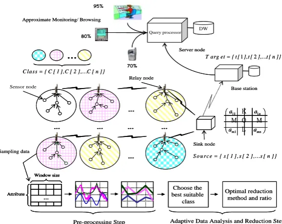
Fig. 1. Overview of real-time data analysis in wireless sensor networks
Many different techniques have been proposed such as clustering, wavelet, histo-gram, regression, aggregation, sampling, principal component analysis (PCA) and singular value decomposition (SVD). Aggregation is an effective way to get a synop-sis (avg, max, min), but is rather crude for applications that need detailed historical information [3, 4]. Spectral models such as discrete wavelet transform (DWT), dis-crete fourier transform (DFT) and disdis-crete cosine transform (DCT) are tuned for time sequences, ideally with a few low-frequency harmonics, but it is ineffective under the multi-dimensional attributes [9, 19]. Sampling has a good overall performance, but is sensitive to the changes in data distribution [15, 19].
Depending on the types of applications that a sensor network is running and the types of data the application is generating, different reduction techniques may have to be employed. In this work, we introduce a framework that adaptively chooses differ-ent reduction strategies based on the classification of the data in each window. The techniques surveyed in this section were evaluated in the context of this adaptive framework.
3 Multivariate Stream Data Classification
3.1 Preprocessing Step
The sensor data generated from such a sensor node collectively forms a multivariate data stream. Each sensor node temporarily accumulates the sensor data and periodi-cally sends it to the parent node in the upper layer. The parent node then collects data transmitted from children nodes and either relays it up to the chain (e.g., from gate-way node to sink node), or store them in the repository or feed them to the application for further processing (server node). Data reduction is typically considered in the transmission between the sink node (Fig. 1) and the base station because the size of data aggregated from children nodes can be large and depending on the applications often times the large, exact original data is out of favor to the compact approximate summarization. Data reduction may also be considered in the server node where all the sensor data is eventually stored for a long-term analysis of historical sensor data.
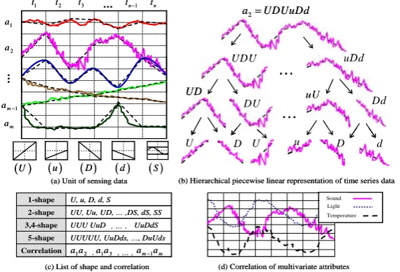
Fig. 2 shows the preprocessing step for our multivariate data classification. In this step, the continuous sensor stream is transformed into the combinations of discrete symbols which represent signal changes such as upward (U for steep inclination and
u for moderate inclination), downward (D for deep and d for moderate) or stable (S) for a given time interval (tk – tk-1). This transformation greatly reduces the complexity of the raw data while retaining the structure of the time series data. For fast trend analysis and pattern matching, we use a hierarchical piecewise linear representation [13] and n-gram model [15] which together can represent various different types of multivariate stream data. In this paper, we used the five character shapes (U, u, D, d,
and S) as shown in Fig. 2(a). All the attributes in a window can be represented as in Fig. 2(b) using the hierarchical piecewise linear representation.
We extended the original hierarchical piecewise linear representation, which splits the original patterns into a set of disjoint sub-patterns, with n-gram based sliding-window pattern chunking in order to support partial matches and to preserve the or-derings between the sub-patterns.
( )D
( )U ( )u ( )d ( )S
1
t t2 t3 … tn−1 tn
1
a
2
a
1
m
a −
m
a
… …
2
a =UDUuDd
UDU uDd
UD
DU uU
… Dd
U D U u D d
(a) Unit of sensing data (b) Hierarchical piecewise linear representation of time series data
Correlation
UUUUU, UuDds, …, DuUds 5-shape
UUU UuD UuDdS 3,4-shape
UU, Uu, UD, … ,DS, dS, SS 2-shape
U, u, D, d, S
1-shape Sound
Light Temperature
(c) List of shape and correlation (d) Correlation of multivariate attributes 1 3
a a
1 2
a a , , …,am−1am
, …,
Fig. 2(c) shows an example of n-gram based chunking (we use the term n-shape to refer to this technique). Moreover, in order to improve the classification accuracy, we exploit the inter-dependency structure that exists among the sensors (e.g., light and temperature), as illustrated in Fig 2(d). We added the symbols representing the pair-ings of sensors that have a strong correlation (we used 0.6 as a threshold) into the list of transformed n-shape symbols as shown in the last row of Fig. 2(c). For example, if sensor a1 and a2 are correlated we add a word, “a1a2 ”, to the shape list. Once the data is transformed, we can simply treat them as a string of words and apply text classification algorithms to classify the data. In what follows, we will describe the details of the classification algorithms that we considered in our framework.
3.2 Supervised methods
NBM (Naïve Bayes Model): Bayesian classifiers are statistical classifiers and have exhibited high accuracy and speed when applied to a large database [15]. This tech-nique chooses the highest posterior probability class using the prior probability of training data set. In this paper, input data is n-dimensional vector which consists of shape sequence for each attribute and correlation values. An example of input data is {e.g., Uu, uDDs, , etc.}. In the training phase, it learns the prior probability dis-tribution such as, P(
1 2
a a
uD | class=" intrusion") and P( a a | class1 2 =" normal"), from the training data. In the test step, for each unlabeled window, a posterior probability is evaluated for each class , as shown in (1). The test data is then assigned to class for which
i
C Ci
i
P( C | X ) is the maximum.
i i
i
P( X | C )P( C ) P( C | X )
P( X )
= , where
1
n
i k
k
P( X | C ) P( x | C )
=
=
∏
i (1)SVM (Support Vector Machine): This method is one of the most popular supervised classification methods. SVM is basically two-class classifier and can be extended for the multi-class classification (e.g., combining multiple one-versus-the-rest two-class classifiers). In our model, each window is mapped to a point in a high dimensional space, each dimension of which corresponds to a shape or a correlation pair. The coordinates of the point are the frequencies of the shapes and correlation coefficients of the correlation pairs in the corresponding dimensions. SVM learns, in the training step, the maximum-margin hyper-planes separating each class. In testing step, it clas-sifies a new window by mapping it to a point in the same high-dimensional space divided by a hyper-plane learned in the training step. For experiments, we used the Radial Basis Function (RBF) kernel [16], 2
(
)
0
i i
x y i i
K( x ,y ) e= −γ − ,γ> . The soft margin
3.3 Unsupervised Methods
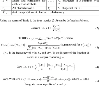
String-based Distance: This scheme measures the distance between two strings in order to measure the similarity. We can obtain the best matching class by comparing the shape and correlation feature vectors of each known class with that of input data. Among many possible distance measures, we used two token-based string distance (Jaccard and TFIDF) and two edit-distance-based ones (Jaro and Jaro-Winkler) that were reported to give a good performance for the general name matching problem in [18]. We briefly describe the metrics below. For details of each metric, refer to [17].
Table 1. Terms for string-based distance
Name Descriptions Name Descriptions
x,y Shape and correlation for each sensor attribute.
x , y
CC All characters in x common with
y
x
C All characters ofx. Tx All shape list for x.
x ,y
X # of transpositions of char in x relative to y
Using the terms of Table 1, the four metrics (2-5) can be defined as follows.
Jaccard (x,y) = x y
x y
T T
T T
∩
∪ (2)
TFIDF (x,y) = ( )
(
)
x y x
w T∈ ∩TV w,T ×V w,Ty
∑
, where( )
(
)
( )(
)
( )(
)
1
1 y
' y
w
x w,T
w,T w
w
log IDF V w,T log TF
log TF log IDF
= + ×
+ ×
∑
(symmetrical for V w,T(
y)
),is the frequency of w in , and x
w,T
TF Tx IDFw is the inverse of the fraction of
names in a corpus containing . w
(3)
Jaro (x,y) = 1
3 2
x ,y y ,x x ,y CC ,CC x ,y y ,x
x y x ,y
CC X
CC CC
C C CC
⎛ − ⎞
⎜ ⎟
× + +
⎜ ⎟
⎝ ⎠ (4)
Jaro-Winkler (x,y) = ( )
(
4)
(
1 ( ))
10max L ,
Jaro x, y + × −Jaro x, y , where Lis the
longest common prefix of xand y
(5)
4 Multivariate Data Reduction Techniques
strategies that are appropriate to the given window. In this section, we describe vari-ous reduction techniques that we considered for our framework.
DWT (Discrete Wavelet Transformation): DWT is a linear signal processing tech-nique using a hierarchical decomposition function. DWT is closely related to the DFT (Discrete Fourier Transform) and performs well with a low frequency data type. It will not perform well if the input signals have spikes or abnormal jumps [9, 15, 19]. The hierarchical pyramid algorithm is generally used for halving the data at each iteration. DWT is generally fast ( for an input vector of length n) and requires only a small amount of space.
( ) O n
HCL (Hierarchical Clustering): Clustering can be used for data reduction as a group of similar objects in a cluster can be replaced with a single centroid. In particular, we used hierarchical clustering method. This method uses the greedy, bottom-up ap-proach, and constructs hierarchical clusters using single, average and complete-linkage method [15].
Sampling:Different types of sampling can be applied such as reservoir sample [19], cluster sample and stratified sample. An advantage of sampling for data reduction is that the cost of obtaining a sample is proportional to the size of the sample. The com-plexity of sampling is potentially linear and we can easily control sampling rate ac-cording to the error ratio.
SVD (Singular Value Decomposition): SVD is a powerful technique in matrix com-putation and analysis (e.g., solving systems of linear equation, pattern recognition, data compression and matrix approximation) [20], which is defined as follows:
Given an m×n real matrixX , we can express it as X= ∑U VTwhere and V
are column-orthonormal matrices containing left and right principal components (their column vectors), is a diagonal matrix containing singular values in a decreas-ing order. Sdecreas-ingular values capture the variation of the input data along the direction of corresponding principal components. Hence, smaller singular values and their corre-sponding principal components typically represent the noise in the data. Using only k
largest components and singular values, we can compute a matrix
U
∑
'
X which is a best rank-k approximation of the original matrixX . In our framework, thus, only top-k
components and singular values are retained for transmission and storage.
5 Experimental Results
5.1 Data Set
(one of sine, cosine, square, triangular and saw-tooth), frequency (in Hz), DC level and random noise.
(a) (b) (c) (d) (e) (f) (a) (b) (c) (d) (e) (f)
(a) Six different time series data (b) Random waveform generator
Fig. 3. Data set: SCCTS and digital signal generator
5.2 Classification: Accuracy measure
We performed k-fold cross-validation in order to evaluate the accuracy of each classi-fication method. For the k -fold cross-validation, an input data set (S) is randomly partitioned into k mutually exclusive subsets (S = {S1,S2,…,Sk}) of equal size. Train-ing and testTrain-ing is performed k times. In iteration i, the subset Si is reserved as the test set, and the remaining subsets are collectively used to train the classifier. The accu-racy of the classifier is then the overall number of correct classifications from the k
iterations, divided by the total number of samples in the initial data.
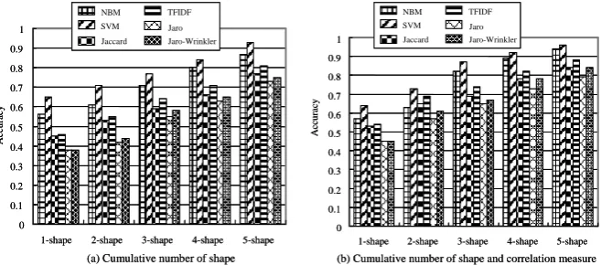
The result of experiments is shown in Fig 4. Fig 4(a) shows the accuracy of the six classifiers discussed in Section 3 using only the n-shape tokens and not considering the correlation tokens (see Fig 2(c).) Fig 4(b) shows the result using both types of tokens. Different lengths of shape tokens are compared. For example, “3-shape” in the x-axis represents the classifications using only shape tokens up to length three (i.e., 1-3 shapes).
0 0.1 0.2 0.3 0.4 0.5 0.6 0.7 0.8 0.9 1
1-shape 2-shape 3-shape 4-shape 5-shape
Ac
cu
ra
c
y
(a) Cumulative number of shape
NBM SVM Jaccard TFIDF Jaro Jaro-Wrinkler 0 0.1 0.2 0.3 0.4 0.5 0.6 0.7 0.8 0.9 1
1-shape 2-shape 3-shape 4-shape 5-shape
Ac
cu
ra
c
y
(a) Cumulative number of shape
NBM SVM Jaccard TFIDF Jaro Jaro-Wrinkler NBM SVM Jaccard TFIDF Jaro Jaro-Wrinkler 0 0.1 0.2 0.3 0.4 0.5 0.6 0.7 0.8 0.9 1
1-shape 2-shape 3-shape 4-shape 5-shape
Ac
cu
ra
cy
(b) Cumulative number of shape and correlation measure
NBM SVM Jaccard TFIDF Jaro Jaro-Wrinkler 0 0.1 0.2 0.3 0.4 0.5 0.6 0.7 0.8 0.9 1
1-shape 2-shape 3-shape 4-shape 5-shape
Ac
cu
ra
cy
(b) Cumulative number of shape and correlation measure
NBM SVM Jaccard TFIDF Jaro Jaro-Wrinkler NBM SVM Jaccard TFIDF Jaro Jaro-Wrinkler
As expected, the accuracy was gradually improved as longer shape tokens were taken into consideration. The longer tokens are likely to capture more temporal local-ity of patterns. The accuracy was generally higher when the correlation tokens were used along with the shape token. Noticeable improvements were observed in 3 and 4-shape experiments as shown in the figure.
Comparing supervised and unsupervised methods, supervised methods (NBM and SVM) were more accurate than unsupervised methods. SVM showed the best per-formance among the tested methods. Among the unsupervised methods, classifiers using token-based string distance metrics were more accurate than the ones using edit-distance metrics. For this experiment, we used the classification library and package provided by [22, 23].
5.3 Data Reduction: Data Type vs. Error Ratio
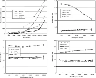
Different reduction methods may have different performance characteristics over different types of data. In our adaptive framework, we choose the best reduction strat-egy for each window according to the classification result for the window. To be able to choose appropriate methods for a particular class, we need to know which reduc-tion method performs well on the windows of which class. Our adaptive framework learns such associations by evaluating different reduction methods over the training dataset. The evaluation result is presented in Fig 5. In the experiment, we compared the four reduction methods discussed in Section 4. The algorithms were implemented using the standard algorithms provided by [24, 25].
The first graph (top left) shows the execution times of each method. Sampling was the best performer in this test for the obvious reason, while DWT was the worst. The remaining three graphs show the performance of the methods in terms of the amount of information lost during the reduction. We used the following metric to measure the relative error (σ) incurred by the reduction.
µ F F
A A
A
σ= − , where
(
)
1 2 2
ij
F ij
A = ∑ a (7)
where A is the original matrix and µA is the approximation of A recovered (decom-pressed) from the reduction of the original matrix. For example, µA can be computed by the interpolation of samples if sampling was used. If SVD was used, µA can be computed by multiplying left and right top-k principal components scaled by the singular values.
0 2000 4000 6000 8000 10000 12000
400 1600 6400 19200 44800 102400 230400 512000 Data Set Size
E x ec ut ion T im e (m il li se conds ) Wavelet HCL Sampling SVD 0 2000 4000 6000 8000 10000 12000
400 1600 6400 19200 44800 102400 230400 512000 Data Set Size
E x ec ut ion T im e (m il li se conds ) Wavelet HCL Sampling SVD Wavelet HCL Sampling SVD 0 0.03 0.06 0.09 0.12 0.15
400 6400 19200 44800 102400 Low-Frequency Data Set
R elativ e E rro r R atio Wavelet HCL Sampling SVD 0 0.03 0.06 0.09 0.12 0.15
400 6400 19200 44800 102400 Low-Frequency Data Set
R elativ e E rro r R atio Wavelet HCL Sampling SVD Wavelet HCL Sampling SVD 0 0.1 0.2 0.3 0.4 0.5
400 1600 6400 19200 44800 102400 High Frequency Data Set
R el ati v e E rro r R at io Wavelet HCL Sampling SVD 0 0.1 0.2 0.3 0.4 0.5
400 1600 6400 19200 44800 102400 High Frequency Data Set
R el ati v e E rro r R at io Wavelet HCL Sampling SVD Wavelet HCL Sampling SVD 0 0.1 0.2 0.3 0.4 0.5
400 1600 6400 19200 44800 102400 Mixed Frequency Data Set
R elativ e E rror R atio Wavelet HCL Sampling SVD 0 0.1 0.2 0.3 0.4 0.5
400 1600 6400 19200 44800 102400 Mixed Frequency Data Set
R elativ e E rror R atio Wavelet HCL Sampling SVD Wavelet HCL Sampling SVD
Fig. 5. Comparing data reduction methods (data types vs. error ratio)
6 Conclusions
In this paper, we proposed an adaptive framework for sensor network data classifi-cation and reduction. For classificlassifi-cation, we employed the hierarchical piecewise lin-ear representation to transform the continuous sensor streams into a discrete symbolic representation, which allows us to choose a classifier from a large pool of well-studied classification methods. We tested four different data reduction techniques over a set of input data with different data characteristics. SVM performed the best in our classification test while SVD and Sampling were the best performers in the reduc-tion test.
References
1. D. Barbara, and W. DuMouchel, et al.: The New Jersey Data Reduction Report, Data Engi-neering Bulletin (1997)
3. A. Deligiannakis, Y. Kotidis, and N. Roussopoulos.: Compressing Historical Information in Sensor Networks. In ACM-SIGMOD (2004)
4. A. Deligiannakis, Y. Kotidis, and N. Roussopoulos.: Hierarchical in-Network Data Aggrega-tion with Quality Guarantees. In EDBT (2004)
5. A. Mainwaring, and J. Polastre, et al.: Wireless Sensor Networks for habitat monitoring. In WSNA (2002)
6. B. Xu, and O. Wolfson.: Time-Series Prediction with Applications to Traffic and Moving Objects Databases. In MobiDE (2003)
7. R. Cardell-Oliver, and K. Smettem, et al.: Field Testing a Wireless Sensor Network for Reactive Environmental Monitoring. In ISSNIP (2004)
8. Y.Chen, and G. Dong, et al.: Multi-Dimensional Regression Analysis of Time-Series Data Streams. In VLDB (2002)
9. F. Korn, H.V. Jagadish, and C. Faloutsos.: Efficient Supporting Ad Hoc Queries in Large Datasets of Time Sequences. In ACM-SIGMOD (1997)
10. C. C. Aggrawal, J. Han, and P. S. Yu.: On Demand Classification of Data Streams. In KDD (2004)
11. M. W. Kadous and C. Sammut.: Classification of multivariate time series and structured data using constructive induction. Machine Learning Journal (2005)
12. P. Geurts.: Pattern Extraction for Time Series Classification. PKDD (2001)
13. Xianping Ge.: Pattern Matching in Financial Time Series Data. In Final Project Report for ICS 278 UC Irvine (1998)
14. R. Agrawal, G. Psaila, E. L. Wimmers, and Mohamed Zait.: Querying Shapes of Histories. In VLBD (1995)
15. J. Han, and M. Kamber.: Data Mining Concepts and Techniques. Morgan Kaufmann Pub-lishers (2000)
16. N. Cristianini, and J. Shawe-Taylor.: An Introduction to Support Vector Machines. Cam-bridge University Press (2000)
17. W. W.Cohen, P. Ravikumar, and S. Fienberg.: A Comparison of String Distance Metrics for Naming-matching tasks. In IIWEB (2003)
18. B.W. On, D.W. Lee, J.W. Kang and P.Mitra.: Comparative Study of Name Disambiguation Problem using a Scalable Blocking-based Framework. In JCDL (2005)
19. M. Garofalakis, and P. B. Gibbons.: Approximate Query Processing: Taming the Tera-bytes! In VLDB Tutorial (2001)
20. G. Strang.: Introduction to Linear Algebra, 3rd Edition, Wellesley-Cambridge Press (1998) 21. Hettich, S. and Bay, S. D.: The UCI KDD Archive [http://kdd.ics.uci.edu]. Irvine, CA:
University of California, Department of Information and Computer Science (1999) 22. A Library for Support Vector Machines: http://www.csie.ntu.edu.tw/~cjlin/libsvm
23. SecondString (Jave-based Package of Approximate String-Matching): http://secondstring. sourceforge.net
24. JAMA: A Java Matrix Package: http://math.nist.gov