ABSTRACT
BIRGE, BRIAN K. A Computational Intelligence Approach to the Mars Precision Landing Problem. (Under the direction of Dr. Gerald D. Walberg.)
Various proposed Mars missions, such as the Mars Sample Return Mission (MRSR) and the Mars Smart Lander (MSL), require precise re-entry terminal position and velocity states. This is to achieve mission objectives including rendezvous with a previous landed mission, or reaching a particular geographic landmark. The current state of the art footprint is in the magnitude of kilometers. For this research a Mars Precision Landing is achieved with a landed footprint of no more than 100 meters, for a set of initial entry conditions representing worst guess dispersions.
Obstacles to reducing the landed footprint include trajectory dispersions due to initial atmospheric entry conditions (entry angle, parachute deployment height, etc.), environment (wind, atmospheric density, etc.), parachute deployment dynamics, unavoidable injection error (propagated error from launch on), etc. Weather and atmospheric models have been developed.
The purpose of this study is to examine the feasibility of using a computational intelligence strategy to facilitate precision planetary re-entry, specifically to take an approach that is somewhat more intuitive and less rigid, and see where it leads. The test problems used for all research are variations on proposed mars landing mission scenarios developed by NASA.
A relatively recent method of evolutionary computation is Particle Swarm Optimization (PSO), which can be considered to be in the same general class as Genetic Algorithms. An improvement over the regular PSO algorithm, allowing tracking of non-stationary error functions is detailed. Continued refinement of PSO in the larger research community comes from attempts to understand human-human social interaction as well as analysis of the emergent behavior.
Using PSO and the parafoil scenario, optimized reference trajectories are created for an initial condition set of 76 states, representing the convex hull of 2001 states from an early Monte Carlo analysis. The controls are a set series of bank angles followed by a set series of 3DOF thrust vectoring. The reference trajectories are used to train an Artificial Neural Network Reference Trajectory Generator (ANNTraG), with the (marginal) ability to generalize a trajectory from initial conditions it has never been presented. The controls here allow continuous change in bank angle as well as thrust vector. The optimized reference trajectories represent the best achievable trajectory given the initial condition. Steps toward a closed loop neural controller with online learning updates are examined.
This is controlled from a MATLAB shell that directs the optimization, learning, and control strategy.
A Computational Intelligence Approach to the Mars Precision Landing Problem
by
Brian Kent Birge III
A dissertation submitted to the Graduate Faculty of North Carolina State University
in partial fulfillment of the requirements for the Degree of
Doctor of Philosophy
Aerospace Engineering
Raleigh, North Carolina 2008
APPROVED BY:
___________________________ ___________________________ Dr. Larry Silverberg Dr. Paul Ro
___________________________ ___________________________
Dr. Mark White Dr. Gerald Walberg
DEDICATION
BIOGRAPHY
Brian “Chip” Birge was born on July 31st, 1969 in Town & Country, MO, USA. He graduated from Indiana’s Purdue University with a Bachelor’s in Physics as well as a Bachelor’s in Electrical Engineering, with a minor in Mathematics. He served two terms as IEEE Student Chapter President.
In 1998 he was accepted into the Aerospace Engineering PhD program at North Carolina State University, and became a graduate research assistant with the Mars Mission Research Center.
He has published research having to do with imaging, Particle Swarm Optimization, space situational awareness, and space object identification and characterization. He has been on research teams studying planetary science, satellite dynamics, nonlinear optimization, robotics, and optics.
Currently he resides in Houston, Texas with his wife Kwan and daughter Rachel and is employed as a principal systems engineer NASA’s Johnson Space Center working on various manned and robotic space exploration projects. His research activities continue to focus on applied and theoretical computational intelligence, high performance computing, and simulation & modeling.
ACKNOWLEDGEMENTS
There are several people over the years that provided me with the help and inspiration to complete this research. Some know it, others do not.
My advisor Dr. Gerald Walberg wins the patience of Job award. Thanks Jerry for your tremendous insight into everything from orbital mechanics to good beer, a font of wisdom and kindness throughout my years of research.
Dr. Russell Eberhart, co-inventor of PSO and my Master’s advisor whose infectious enthusiasm for the subject got me excited about computationally emergent behavior and research in general.
Astronomers, the late Dr. John Africano who made pure science fun and Dr. Doyle Hall, whose rigorous approach to real problems is a model I try to follow.
Finally, I especially appreciate the staff of the MAE department and graduate school for their excellent support throughout my time at NCSU.
TABLE OF CONTENTS
Page
LIST OF TABLES....………..……..ix
LIST OF FIGURES………..………..x
LIST OF SYMBOLS AND ACRONYMS……….xiii
INTRODUCTION……….……….1
BACKGROUND………4
Viking EDL………5
Pathfinder/MER EDL……….8
Mars Science Laboratory EDL………..…...12
Mars Precision Lander EDL……….15
Summary of Past Missions and Current State of the Art……….16
TOOLS……….18
MATLAB Introduction………18
Program to Optimize Simulated Trajectories (POST)….………19
MarsGRAM………..20
MISSION DEVELOPMENT………...22
Scenario Study………..22
Baseline………23
Thrust on a Ballistic Parachute……….26
Hover and Thrust Laterally………..28
Summary of Scenario Study……….34
Environment……….35
Standalone models………35
Atmosphere………..36
Winds & Gusting……….38
Gravity……….40
Topography Sensor………..41
POST Models………...42
MPL Input Deck………...43
TRAJECTORY OPTIMIZATION………...46
First Guesses with POST……….47
Results of First Guess Study………...49
PSO Primer………..49
PSO for Changing Environments………51
Training set order reduction……….53
Cost Function……...………54
Multi-objective Optimization………...56
Terms of the Cost Function………..57
Results………...………...59
ARTIFICIAL NEURAL NETWORK TRAJECTORY GENERATOR…...………...62
Neural Network basics……….………62
Validation Problem 1………...64
Validation Problem 1, Results………..68
Validation Problem 2………...69
Validation Problem 2, Results………..76
Validation Study Conclusions……...……….………..78
ANNTraG………79
Discrete………79
Continuous………...81
Interpolation………84
Open Loop Control………..85
CONCLUDING REMARKS………...89
RECOMMENDATIONS FOR FUTURE WORK………..91
Closing the Loop……….91
Online Update of the Neural Network Controller………..….91
Hazard Avoidance………...92
REFERENCE MATERIALS………...94
APPENDICES……….97
Appendix A – Particle Swarm Optimization (PSO)...………..98
Overview………..98
PSO Algorithm Details……….99
Matlab Toolbox Usage………...102
Appendix C - Generic POST Input Deck used in Control System………116
Appendix D - Cost Function used in Trajectory Optimization Runs……….127
Appendix E - Routine to Build Partial POST input decks……….135
LIST OF TABLES
Table 1 Mission Details for Past and Proposed Mars Missions………....17
Table 2 Convergence Success for Hover and Thrust Laterally...29
Table 3 Distance Breakdown for Trajectory Optimization...61
Table 4 Validation Problem 1, Target Errors...68
Table 5 Initial Conditions in Planet Relative Coordinates...70
LIST OF FIGURES
Figure 1 Viking Orbiter/Lander Mission Scheme...6
Figure 2 First panoramic view returned of Mars, Viking 1………...7
Figure 3 MPF EDL Strategy...9
Figure 4 DIMES in action...12
Figure 5 MSL EDL...14
Figure 6 MSL Sky Crane Maneuver...15
Figure 7 MPL EDL...16
Figure 8 Handoff condition subset with Baseline landed ellipse………...25
Figure 9 Baseline Scenario Propellant Used...26
Figure 10 Initial and Final ellipses for the Thrust on the Parachute case……….27
Figure 11 Thrust on the Parachute Fuel Consumption……….28
Figure 12 Handoff to Hover Ellipse...30
Figure 13 Hover and Thrust Laterally, Landed Ellipse………....31
Figure 14 Hover and Thrust Laterally Propellant Usage………..32
Figure 15 MPL Landed Ellipse………...33
Figure 16 MPL Propellant Usage………...34
Figure 17 Standalone Mars Environment Model Integration………...36
Figure 18 Mars Atmosphere Model, Glenn Research Center type………...37
Figure 19 Mars Northerly Winds as a function of Altitude & Time………....39
Figure 21 Deviation from mean geoid surface height along 3 trajectories…………...42
Figure 22 Autonomously Steered Parafoil drop test………...44
Figure 23 First Guess Geometry...48
Figure 24 Reduction of Initial Conditions...53
Figure 25 PSO Trajectory Optimization Run...60
Figure 26 Trajectory Optimization Results...60
Figure 27 Generalized Schematic of an ANN...63
Figure 28 Neural Training Set for Validation Problem 1………...67
Figure 29 Validation Problem 1, Impact Points...69
Figure 30 Reachable Ground Impact points for Validation Problem 2………....71
Figure 31 Curve fit of Reachable Impact Points, 17km Altitude...73
Figure 32 Curve fit of Reachable Impact Points, 13km Altitude………...74
Figure 33 Curve fit of Reachable Impact Points, 9.5km Altitude………....74
Figure 34 Training Data overlayed with Neural Net derived Data………...76
Figure 35 Validation Problem 2, Impact Points...78
Figure 36 Open Loop Control on Known Trajectory...86
Figure 37 Open Loop Control on Known Trajectory #2...88
Figure 38 Conceptual closed loop approach………92
Figure 39 Fidelity of Topographic Sensor with currently available Data…………....93
Figure 40 Schaffer f6 function...102
Figure 41 Schaffer f6 over the range [-100,100]...106
LIST OF SYMBOLS AND ACRONYMS
INTRODUCTION
There is a renewed interest by the public in space exploration, sparked by such successes as the Mars Pathfinder and Orbiter missions. As engineers, each success asks us to push the boundaries a little more on the next project. It is a truism that to find the boundaries of a thing that thing must be broken. We inch forward passing incremental boundaries, each progress building on the previous. Seemingly endless pre-analysis and post-analysis by teams of qualified people dedicated to each project give us high confidence of mission achievement but even so, events happen that deviate from prediction. What can we do when a spacecraft encounters a scenario not envisioned by the mission planners? There exists a real need for adaptive control in a newer sense, not only should the system adapt to changing parameters but it should be able to modify its behavior.
The purpose of this study is to examine the feasibility of using a computational intelligence approach to facilitate precision planetary re-entry from the beginning of the Entry, Descent, Landing (EDL) phase through touchdown. The test problems used for all research are variations on proposed mars landing mission scenarios developed by NASA.
avoidance, precision landings, active downrange and crossrange guidance, re-tasking, and resistance to atmospheric and environmental dispersion.
A baseline MRSR style mission would consist of a two tiered approach. First, a ship is sent to Mars and drops a Lander on the surface. This Lander performs some basic science tasks, among them collecting geologic samples. Rather than send a whole robotic geology laboratory to Mars to analyze the samples (a current impossibility), a second spacecraft is then sent to pick up the sample. This scenario requires the second Lander to precisely match the location of the first Lander to within some engineering capable tolerances. To make the scenario conceptually even simpler, imagine a single spacecraft sent, but this time the science team is keen on examining a very specific feature on the planet, perhaps in the middle of some very rough terrain. The technologies that would make such a Precision Landing possible now seem very desirable.
Given the current state of robotic rovers, a Mars Precision Landing requirement is desired with a landed footprint of no more than 100 meters from a target [2]. In contrast, the Viking mission had a landing footprint of over 100 kilometers (excellent for that particular mission requirement). The current state of the art’s footprint is still in the magnitude of kilometers [4].
research to reduce the simulated landing footprint to target to 100m and significantly closer in some cases.
In recent years, a number of computational techniques that lend themselves particularly well to control problems have become available. In broad categories they are Fuzzy Systems (FS), Artificial Neural Networks (ANN), and Evolutionary Computation (EC). Fuzzy Systems are based on fuzzy logic which is in turn based on the way our mind deals with incomplete and/or inaccurate information. Neural Nets are modeled after the spatial structure of the brain and allow ‘connectionist’ learning properties. Evolutionary computation paradigms such as Genetic Algorithms (GA) and Particle Swarm Optimization (PSO) are loosely modeled after biological evolution and optimization. These techniques have been shown individually to work very well in solving a large number of problems in linear and nonlinear system identification, modeling, and control [20].
Until recently FS, ANN, and EC were totally separate fields with very little interaction. A growing number of researchers and practical engineers are discovering that a combination of two or more of these methods offers advantages that a single one lacks.
Using an ANN in a control system we add fault tolerance, distributed (connectionist) representation properties, and the ability to learn optimal responses to new input. If we add an FS ‘shell’ we include high level rule/decision abilities as well as comparative reasoning. Combining techniques this way is called Computational Intelligence (CI).
BACKGROUND
Motivation for the current work springs from several areas. Historically, touchdown requirements for missions to Mars have been ‘loose’. That is, the designers and mission planners were more interested in getting to Mars with a functioning vehicle than in reaching a particular geographic location. As long as the terminal velocity conditions were met and the rather large dispersion footprint was adhered to then the design was a success.
Out of the five successfully delivered robotic Mars exploration missions, all had masses below 600kg and landed at geographic positions below -1km Mars Orbiter Laser Altimeter (MOLA) average elevation in order that the entry, descent, and landing system could perform with enough atmospheric density. Also, they all had landed footprints on the order of 100km [4].
descent phase refers to the the period starting from initial parachute deployment to first touchdown.
Viking-era EDL
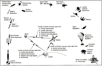
The first landing standard was that of the Viking Planetary Lander. The mission was planned with two separate landed vehicles, each with autonomous navigation, guidance and control. Each of the two missions consisted of an Orbiter and a Lander. The Orbiter scanned the surface from orbit, looking for suitable places for touchdown. It also scanned for surface moisture and temperature readings as part of the search for life. Once a suitable area was found, the Lander was powered on and received a state update from the orbiter. About 30 hours later (to give time to check out the descent instrumentation), the Lander separated from the orbiter.
After separation, the Lander was rotated into position for the deorbit maneuver. After deorbit, the Lander went into a coast mode until atmospheric entry at 224km above mean surface level. This was determined by a set wait time, rather than any atmospheric sensing. It was designed such that there was approximately 7 to 10 minutes before touchdown on the surface. At the start of this 7-10 minute block, the Lander’s flight computer fully powered up from sleep mode and the Lander was oriented by the Reaction Control System (RCS) such that the heat shield was positioned to meet the atmosphere. The Lander’s re-entry speed at this time was about 4.6 km/s [18].
followed eight seconds later. 45 seconds after that at approximately 1.49km altitude and 66m/s velocity magnitude, the parachute cover was discarded. At this time, the retro rockets were ignited and individually throttled to affect pitch, yaw and terminal velocity. Engine shut off happened when the legs touched the surface via shock sensor. The nominal velocity at this time was designed to be approximately 2.44 m/s.
Figure 1. Viking Orbiter/Lander Mission Scheme
On June 19, 1976 Viking 1 touched down at Chryse Planitia (22.48° N, 49.97° W). Two months later on August 7, 1976 Viking 2 touched down at Utopia Planitia (47.97° N, 225.74° W). The Viking Landers sent back images of the surface, dug surface samples analyzing them for signs of life, installed seismometers, and perhaps most important for this study, they examined atmospheric composition and meteorology. It is the advances in Martian meteorology made by scientists analyzing Viking data that allow a much clearer picture of the regime in which future missions must perform. The Viking 2 Lander ended communications on April 11, 1980, and the Viking 1 Lander followed suit on November 13, 1982.
Figure 2. First panoramic view returned of Mars, Viking 1
The spaceship landed basically where the scientists wanted it (give or take a 100 km), nothing was broken. However, if the Lander had encountered a dust devil (not known at the time) or a dust/sand storm (a real concern to the scientists) during re-entry then things may have gone very differently. The Lander could not re-task itself in the face of unexpected input. Additionally, the landing sites were chosen because they were expected to be free from extensive obstacles, at the trade off of being less geologically interesting than other proposed sites. With the ability to re-task during descent theoretically obstacles can be avoided, surprises can be mitigated, more interesting sites can be explored, and the Precision Landing problem can be tackled. Studies have shown that as successful as the Viking missions were, the EDL strategy will be too limiting for future Precision Landing requirements [3].
Pathfinder/MER EDL
The next advances in Mars EDL guidance came with the Mars Pathfinder Lander (MPL) and Mars Exploration Rover (MER) missions. Both Pathfinder and the MER mission had many legacy elements to the terminal descent phase, borrowing heavily from Viking based technology.
motivated by a need for cost savings when compared to the earlier Viking mission but it also took concepts from previous lunar landers and US Army payload delivery systems [28].
The Pathfinder EDL, like Viking was an autonomous rigid series of maneuvers that was triggered by a start command from mission control on Earth. The Pathfinder had direct uncontrolled (except for stability) ballistic entry that was followed by a ballistic parachute descent and an airbag bounce landing that borrowed from an earlier Russian post-Apollo era concept [9].
After a spin controlled ballistic entry by a Viking style aeroshell allowed the martian atmosphere to decelerate the lander from 7.5 km/s to 400 m/s. At that time the EDL phase began. A 12.5m diameter non-maneuverable parachute was designed to be deployed at between 5 and 11 km altitude to slow the vehicle even further. 20 seconds later the heatshield was jettisoned and the lander began to separate from the backshell by sliding down 20m worth of bridle (metal tape), looking at this point much like a flying pendulum. Then the radar altimeter was activated and acquired the surface about 32 seconds before touchdown at an altitude of 1.5km. 8 seconds and 300m above the surface, the airbags inflated. At 100m above the surface, the backshell ignited a quick burst of retro rockets to slow the velocity down to near zero. At this point the lander was hanging onto the bridle with airbags inflated and was about 12m above the ground. The bridle was cut and the lander protected by airbags, fell to the surface, bounced a bit and that was that.
On July 4, 1997 Pathfinder made its descent to Mars with a 23km touchdown from nominal, well within the designed 300km by 100km touchdown ellipse science requirement.
In contrast with Pathfinder, the MER missions A and B were developed in the atmosphere of change created by the failure of the 1999 Mars missions. The missions were designed to take advantage of the favorable 2003 launch opportunity and therefore the time from development to launch was a mere 35 months. This meant that the schedule was a significant challenge.
Figure 4. DIMES in action
In early 2004, both MER missions successfully landed the robotic explorers Spirit and Opportunity.
Mars Science Laboratory EDL
Laboratory (MSL) incorporates a much more sophisticated design than the previous landed missions.
Like Viking, the MLS entry vehicle will fly at an angle-of-attack so that it will have a small lift. Another big change is that MSL will be the first lander to have an autonomous guidance system that can detect and adjust for hazards, allowing a richer set of landing position candidates. The MSL entry vehicle has an offset center of mass designed to allow it to hit atmosphere at a 16 degree angle of attack and have a 19 degree angle of attack at the point of parachute deployment [4]. The angle of attack creates lift and during the initial atmospheric entry, the vehicle will be bank angle adjusted (steered) to drive down entry dispersion errors and reach the desired parachute deployment point. A Reaction Control System (RCS) with retro rockets will adjust the bank angle during this phase.
Figure 5. MSL EDL
Because of the expected tight altitude window for this mission the engines will throttle up within 2 seconds of parachute jettison. The rockets are throttled to provide gentle vertical descent of 0.75 m/s. During this phase, the lander is lowered via 3 bridles in a procedure known as the Sky Crane maneuver. This two body system allows a closed loop control all the way to touchdown. When the touchdown is sensed, the upper stage cuts loose the lander and fires lateral rockets to avoid coincident impact.
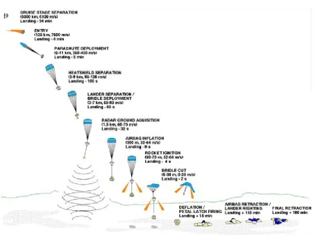
Mars Precision Lander (MPL) EDL
The proposed technology of this research is the Mars Precision Lander (MPL). This will carry on the tradition of using Viking and later derived concepts and adding a few new twists.
data and retraining the neural net. The rest of this paper will explain the MPL EDL strategy in more detail.
Figure 7. MPL EDL
Summary of Past Missions and Current State of the Art
Table 1. Mission Details for Past and Proposed Mars Missions Landing Year:
Mission:
1976 Viking 1
1997 MPF
2004 MER A
2010
MSL plan MPL sim
Entry Mass kg 992 584 827 2800 2200
Lift to Drag ratio 0.18 0 0 0.22 1*
Parachute Diam. m 16 12.5 14 19.7 13
Drag Coefficient 0.67 0.4 0.4 0.67 0.4
Chute deploy Mach 1.1 1.57 1.77 2 1.77
Chute Dyn. Pres. Pa 350 585 725 750 585
Chute deploy Alt. km 5.79 9.4 7.4 6.5 9.4
Attitude Control Roll Rate None None Roll Rate Parafoil Roll Descent Vel. Cntrl. Throttle Sep
Cut
Sep Cut Throttle Chute & Throttle Horiz. Vel. Cntrl. Throttle
Pitch
Passive Lateral SRMs
Throttle Pitch
Throttle 3 axis
End Vert. Vel. m/s 2.4 12.5 8 0.75 < 1
End Horiz. Vel. m/s < 1 < 20 11.5 < 0.5 < 1
End Mass kg 590 360 539 1541 1500
Major Axis km 280 200 80 20 0.1
Minor Axis (km) 100 100 12 20 0.1
TOOLS
Matlab Introduction
The majority of the algorithmic work for this research was done with the Matlab programming language. Matlab is a matrix based computer language developed by the Mathworks company. It is interpreted, meaning there is no separate compile step before run. The user can type commands in a terminal window and have them executed immediately. The syntax is very simple to learn yet the language is very powerful, chiefly due to the large amount of toolboxes, or user contributed code extensions. Matlab is used in many contexts, within algorithm development, data analysis, graphical visualization, simulation, engineering and scientific computation, and application development.
The basic data element in Matlab is an array that does not require dimensioning. This allows vectorized code to be developed as well as being intrinsically suited to matrix operations. Unsurprisingly, Matlab stands for Matrix Laboratory and was originally written to provide easier user access to the powerful LINPACK and EISPACK mathematical libraries. The modern versions of Matlab use the state of the art LAPACK and BLAS libraries.
being uploaded to the Mathworks website and is the most downloaded user contributed optimization code [1].
Program to Optimize Simulated Trajectories (POST)
The state generator environment for this research was the Program to Optimize Simulated Trajectories (POST) [27], PC and Unix versions. POST, as used here, is a three degree of freedom, rigid body, point mass simulation program. The program was originally developed to help design the ascent and descent mission designs of the early Space Shuttle project and has been added to and improved upon continuously since. It is used to simulate atmospheric flight mechanics and orbital transfer problems, has an extensive set of weather models, allows powered or unpowered flight simulation, and has reasonably accurate planetary science built-ins. POST was written in Fortran 77 and later modules continue to be written in C. POST II exists with more capability but was not used in this research. Mostly the PC version (basically a beta of POST II) was used. To set up a simulation, POST uses an input deck, a Fortran-like namelist input procedure to define the problem. To help, POST has an integrated set of Flight Control System (FCS) modules as well as discrete parameter targeting and optimization to both equality and inequality constraints.
The planet module defines the environment in which our vehicle will operate. The module consists of an oblate spheroid model, a gravitational model, an atmosphere model, and a winds model.
The vehicle module has typical vehicle properties such as mass properties, propulsion, aerodynamics & heating, airframe characteristics, navigation and guidance models, and a flight control system model.
The trajectory simulation module controls the program cycling by parsing the event sequences. It has table interpolation functions and standard integration techniques which are used to sole the translational and rotational equations of motion.
The trajectory auxiliary calculations module takes care of computed output values, such as conic parameters, ranging, tracking data, and many more.
The targeting/optimization module allows the user to select an optimization variable, dependent variables, and independent variables to solve optimization problems. There are a few optimization methods built in, two gradient descent based and one derivative based, all requiring good first guesses for the chosen variables [20].
For this research, POST was used as the state generator environment while Matlab was used as a control shell.
MarsGRAM
MISSION DEVELOPMENT
Scenario Study
The scenario study part of the research was done early on to decide what kind of EDL mission profile would be best to examine from a Computational Intelligence standpoint. Several ideas were postulated and tested within a stock POST Mars environment state space. Minimal optimization was done with the POST included routines.
For future planetary exploration missions, either robotic or manned, it is desirable to precisely target a lander's touchdown point. Perhaps there has been a previous robotic mission that requires a follow-up robotic mission in order to retrieve collected samples and return them to earth. Perhaps there are specific geographical features that require close-up study. Regardless, a need for precision landing within 100 meters of a specified geographic location exists. Current state of the art can only achieve positioning to within approximately 10 kilometers [4]. This study examines some proposed mission profiles for controlling a lander as it touches down on a specific point on the Mars landscape. All model parameters and constants are taken from and designed to be compatible with the M2001 specifications that were available at the time.
Baseline
The baseline scenario is the simplest. It takes a subset of initial conditions provided from a Monte Carlo study for the Mars 2001 mission [3] and propagates them through the state integrator until touchdown on the surface. This takes the initial conditions, and pops open the parachute to slow down. There is no thrust applied while the parachute is deployed. Once the parachute is jettisoned, the control system kicks in and performs a gravity turn to touchdown. The lander's touch down latitude and longitude is not targeted but ending velocity and altitude conditions are targeted with the built in optimization of POST. This provides the landed footprint ellipse that all other scenarios will try to minimize.
These desired end conditions are:
0.1 <= ur <= 2.1 m/s 0.1 <= vr <= 2.1 m/s
wr = 2.0 m/s 2499 <= gdalt <= 2500m
The relative ground velocity components are ur (N/S), vr (E/W), and wr (up/down). Gdalt is the geodetic altitude. 2500 meters is the surface level above the mean oblate planet spheroid at the mean landed latitude and longitude. As has been previously mentioned, the POST input deck process treats each problem as a series of events.
position and velocity components are input in an inertial coordinate frame from Mars 2001 Monte Carlo analysis. The gravity model is an oblate planet using spherical harmonics from j2 through j6. Guidance is strictly used for gravity turn (velocity null) and uses atmospheric relative aerodynamic angles. There is one engine, pointed out the X body axis.
Event 2 sets the parachute deployment. The parachute is limited to 13 meters diameter and the weight is adjusted for dropping the heatshield.
Event 3 triggers when the parachute is fully deployed. At this point the lander’s surface area is increased to represent the full area of the parachute at 132.73 m2. The drag of the lander is overshadowed by the drag of the parachute so it is ignored. This event simulates the effect of a ballistic parachute.
Event 4 triggers when the lander is 1000m above the surface (+3500m MOLA). At this time the parachute is jettisoned, the vehicle parameters are returned to reflect lander characteristics and the engines are turned on. The internal POST targeting adjusts the thrust and vehicle angle to meet the constraints using relative aerodynamic angles.
Event 5 triggers when the lander is 500m above the surface (+3000m MOLA). This is another opportunity for the POST targeting functions to adjust the controls.
Event 6 is the last task and occurs at surface touchdown. The engine is turned off and the problem is ended.
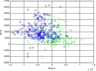
The following figure shows the initial parachute handoff conditions as blue circles and the final touchdown points as green x’s. Both initial and final condition extrema map out to an approximate 20km x 10km ellipse.
-1.5 -1 -0.5 0 0.5 1 1.5
x 104 -3000
-2000 -1000 0 1000 2000 3000 4000 5000 6000 7000
long-m
la
t-m
Figure 8. Handoff condition subset with Baseline landed ellipse
desired conditions and returned garbage. There will be more on the reasons for that in the section about First Guesses.
batch-235(231)pts-bkb3firstguesses-noopt-nothrust
0 50 100 150 200 250
-50 0 50 100 150 200 250
propellant used, m ean=210.5687
trial
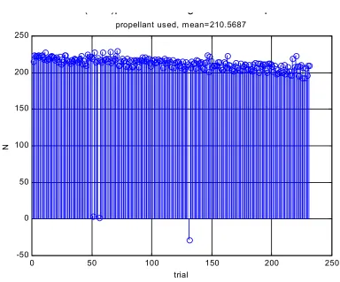
N
Figure 9. Baseline Scenario Propellant Used
Thrust on a Ballistic Parachute
The first candidate scenario examines the effect of thrust vectoring while the parachute is deployed and includes an algorithm for determining targeting initial guesses which will be discussed in another section.
exactly as in the baseline scenario. Targeting is used as in the baseline case but optimization is added on. The range to target is minimized by using the same controls as before but used in slightly different times. There is another event added right after the parachute has fully deployed where the engines turn on and get a thrust command. So, for this case there are three opportunities for optimization of the range. Initial guesses here are starting to get a bit trickier, so fewer initial conditions were able to target. This is a trend that will continue all the way through this section of the research and the solution will be discussed later.
This is now a 15 dimension optimization problem (for each initial condition) where there are 3 events that can receive control commands. The controls are thrust, pitch, pitch rate, yaw, and yaw rate. Or in POST terms (variables) etapc1, pitpc1, pitpc2, yawpc1, and yawpc2. Using the gradient descent POST based targeting and optimization routines 216 out of 235 initial conditions managed to converge to solutions.
batch-235(216)pts-bkb3firstguesses
-8000 -7000 -6000 -5000 -4000 -3000 -2000 -1000 0 1000 -1000
0 1000 2000 3000 4000 5000 6000
initial (blue o) and final ellipse (green x)
long-m
la
t-m
batch-235(216)pts-bkb3firstguesses
0 50 100 150 200 250
0 50 100 150 200 250 300 350 400
propellant used, mean=304.0459
trial
N
Figure 11. Thrust on the Parachute Fuel Consumption
Hover and Thrust Laterally
The second part of the scenario handles from the Hover condition (end of the first deck) down to the surface, taking care of the terminal descent phase. The terminal states of the previous case are used as initial conditions for the next input deck. This scenario is different from the 'thrust on parachute' scenario in that it targets directly to the reference latitude and longitude rather than just trying to minimize the landed distance. There is no first guess algorithm for the optimization. The targeting first guesses assume the reference point is somewhat south of the initial conditions (which indeed it is for most of the points tested). The targeting also starts immediately.
Convergence became an issue with this study. As in the other cases, 235 initial conditions were taken from the full 2000 Monte Carlo point data set, in a random uniform sampling. For the first part of the EDL, the gravity turn, convergence occurred 234 times. For the second part, from hover to touchdown, only 180 out of those remaining 234 converged. The POST included optimization had a very difficult time with this scenario.
Table 2. Convergence Success for Hover and Thrust Laterally Part 1: gravity turn to a hover condition 99% converged Part 2: horizontal thrust & hover to target 76% converged
It should be noted that these cases did not use an algorithm for choosing first guesses for the targeting algorithm in POST. After this portion of the research it was postulated that a first guess algorithm would better targeting results.
batch-235(208)pts-hover20deg.m at
-1.5 -1 -0.5 0 0.5 1 1.5
x 104 -3000
-2000 -1000 0 1000 2000 3000 4000 5000 6000 7000
initial=black diamond, initial end and hover begin=o, final=blue x
long-m
la
t-m
Figure 12. Handoff to Hover Ellipse
The final ellipse is so small (centered at 0 reference) that it is hard to see. Most of the points targeted to within 100 meters. Also, the initial parachute handoff ellipse and the initial hover point ellipse are similar in magnitude with an offset of position. This is expected.
implies less of a science package so a scenario needs to be found that allows large payloads without needing large amounts of fuel.
The graphs below show the focus on the landed ellipse followed by the fuel usage. batch-235(208)pts-hover20deg.mat
-1500 -1000 -500 0 500 1000 1500 2000 2500 -400
-200 0 200 400 600 800 1000
long-m
la
t-m
batch-235(208)pts-hover20deg.mat
0 50 100 150 200 250
0 100 200 300 400 500 600
propellant used, mean=357.5601
trial
N
Figure 14. Hover and Thrust Laterally Propellant Usage Guided, Lifting Parachute (MPL)
The third candidate scenario is the guided, lifting parachute mission (parafoil). This is the scenario that was eventually chosen and has precedent in the X-38 crew escape vehicle project [23]. The POST deck that is described here is slightly different than the one used in the later research. However, for simplicity, they are both referred to as the Mars Precision Lander (MPL) scenario. The main features of the MPL scenario include ballistic entry, ballistic parachute which transforms into a lifting body, then thrusters during the last 1000m meters before touchdown. The chief difference between the MPL incarnations is in the amount of controls and different parachute lift scenarios.
straight flight and the lander glided straight into the target. The terminal descent phase was the same gravity turn as the other scenarios. This approach was able to optimize range to target in similar manner to the hover and thrust scenario but has the advantage of using much less fuel. Again similar to the hover and thrust scenario, the MPL scenario required good first guesses for the optimization algorithm to converge to a solution. Therefore the number of initial conditions that targeted was less than the full set.
The graphs below show the landed ellipse as well as fuel used. The set shown is the set that successfully targeted to the end velocity conditions. A single bank angle turn followed by a glide does not seem to be enough to achieve a full precision landing, however the strategy shows promise. The landed footprint was reduced from +/-15km to +/-1km. It is interesting to note that the final conditions line up more or less along the mean initial velocity vector.
-4 -3 -2 -1 0 1 2
x 104 -1
-0.5 0 0.5 1 1.5x 10
4
long - m
la
t
-
m
0 50 100 150 0
50 100 150 200 250 300 350 400
trial
N
mean propellant used = 231.3451N
Figure 16. MPL Propellant Usage
Summary of Scenario Study
Four scenarios were studied, a baseline case followed by thrust on a ballistic parachute, hover and thrust laterally, and the guided lifting parachute with one turn command. Despite optimization convergence problems on the last two scenarios, they both showed promise as candidate precision landing mission architectures.
Environment
There are several Mars environment models that were developed as part of this research. The environment is a tricky area for the MPL. The goal is to design a system capable of handling wide dispersions in various atmospheric quantities. However, for a real-world representative simulation, a set of accurate environment models are needed. The initial Mars model that was included with POST was a simple low fidelity table lookup with inaccurate wind data. In an effort at improvement, several more detailed models were examined.
Standalone Models
V External U External
Time U noiseV noise W noise Gust/Noise Model Alt g Gravity Model Cd Do Weight Init pos Init Vel Init Acc Constant Parameters Lat Long Alt Time Rho Temp Press
U Wind component
V Wind component Atmosphere Model Rho g Cd Do Weight
External Force U
External Force V
External Force W
Current Vel
pos
vel
accel
3DOF Model
Figure 17. Standalone Mars Environment Model Integration
Atmosphere
The atmosphere model was initially based off of the simple height based model from Glenn Research Center [12]. It is not particularly accurate but it is very simple to code and runs very fast in an engineering simulation.
A high fidelity model covering Helles Basin, Valles Marinares, and the Mars North Pole was developed with data provided by Oregon State University [31]. The OSU data is several gigabytes worth and had never been formulated for use in a real-time simulation before. When they run their models, it takes several days on a large parallel computing cluster to get the results. As of necessity, that data has been pared down considerably for this simulation but the subset still provides the highest fidelity model over the covered local regions.
Figure 18. Mars Atmosphere Model, Glenn Research Center type
in pascals, temperature in Kelvin, atmospheric density in kg/m3, and speed of sound in meters per second.
There is also a simplified call that will use the appropriate Mars model based on the state, OSU for the three localized regions and either Glenn or MarsGRAM for the non-localized data, depending on user input.
Winds & Gusting
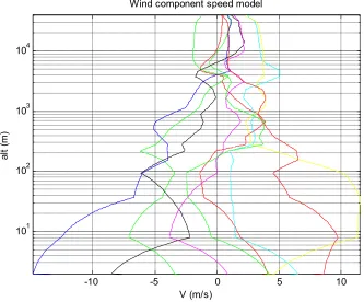
Similar to the atmosphere model, a winds model was created. The model was developed from the OSU data [31] and is strictly valid only for those localized regions. It is a dynamic wind model, covering the changing winds in hour increments for a period of 20 days. For static wind profiles, the latest version of MarsGRAM can also be used. Originally wind table modifiers were used in conjunction with MarsGRAM to correct for model inaccuracies but that has been superseded by newer releases. The dynamic wind profiles, though only valid for North Pole, Helles Basin, and Valles Marinares regions, are used regardless of the latitude and longitude of the vehicle during the simulation. This is because these are the only dynamic wind models in existence and for validation of an engineering model, the interest is in the changing wind profile envelope and how it affects control system performance, as opposed to completely sub-meter accurate location weather dynamics.
In addition to the wind models, there is a simple gusting model that is set as a perturbation of the winds. It is user configurable to specify a gust profile in time and/or altitude or to have random gusts of a maximum strength. The below figures show the dynamic wind profile in 3 hour increments over a single 24 hour period.
-25 -20 -15 -10 -5 0 5 10
101 102 103 104
U (m/s)
al
t
(m
)
Wind component speed model
-10 -5 0 5 10 101
102 103 104
V (m/s)
al
t
(m
)
Wind component speed model
Figure 20. Mars Easterly Winds as a function of Altitude & Time
Because of the timescales during the EDL phase of MPL, the winds can be taken as static to a first approximation. For speed the MarsGRAM POST static wind model was used for the initial runs and the dynamic winds used for higher fidelity simulation.
Gravity
as they would add considerable complexity, computation time, and not be very useful for the purposes of the terminal descent phase.
The inputs to the function are longitude, latitude (only meaningful for an oblate planet), altitude, and model type whether oblate or spheroid mars or earth or custom. If it is a custom planet then radius of the equator, radius at pole, mass factor of planet in earth multiples, and 2nd up to 8th gravitational harmonics. The output is the gravitational acceleration in the ‘down’ direction in meters per second squared. Optional outputs are the gravitational acceleration in inertial coordinate components, the gravitational potential, and gravitational acceleration in spherical coordinate components (deg/s2).
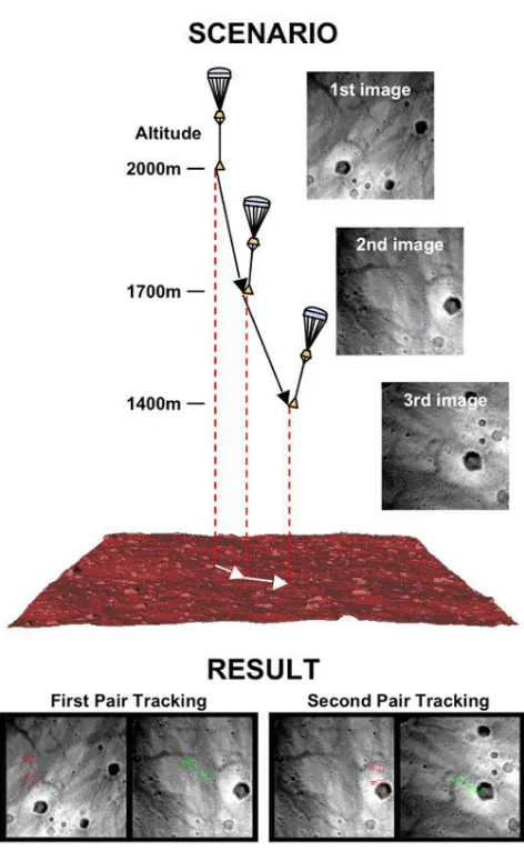
Topography Sensor
0 50 100 150 2700
2710 2720 2730 2740 2750
elapsed time (sec)
m
ar
s
su
rf
ac
e
ab
ov
e
m
ea
n
(m
)
Figure 21. Deviation from mean geoid surface height along 3 trajectories
POST Models
MPL POST Input Deck
This section describes the architecture of the Mars Precision Lander (MPL) POST input deck, as it differs slightly from what was used in the Scenario Study, chiefly in the number of controls. Briefly, the scenario consists of ballistic entry, followed by ballistic parachute to reduce velocity. Then the parachute is converted to a parafoil by severing some tie lines and the vehicle is bank angle steered toward the target. There are 3 steering opportunities. Then the retro rockets are turned on, parachute is jettisoned, and the MPL is controlled for terminal descent with 3 vectored thrusting events.
Event 1, sets initial conditions. Wind table modifiers are input (for the early versions of MarsGRAM). Initial conditions are passed in from a Matlab shell that iterates through a list. The vehicle weight at parachute deploy is 585.479 kg. Propellant weight starts off at 100kg.
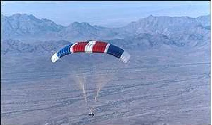
Event 2, deploys the ballistic parachute. The parachute dynamics are set such that it is fully deployed to a 13m diameter in about 3 seconds. The parachute drag coefficient is 0.41.
increasing or decreasing tension on either of the 2 sets of tie lines, the system is able to command bank angle turns. The photo is from the X-38 project [23].
Figure 22. Autonomously Steered Parafoil drop test
Events 4-6, glide on the parafoil using bank angle commands to minimize distance to target. The timing of these events is also an optimization variable.
Event 8, turns on engine when lander is 1000m above MOLA derived surface. Events 9-11, use vectorized thrusting to minimize both range to target and touchdown velocity. Timing of each of the three events is also an optimization variable.
Event 12, touchdown and end program.
TRAJECTORY OPTIMIZATION
The idea behind trajectory optimization is to find the set of controls that will optimize the range to our target as well as meet the terminal conditions of minimal velocity. The terminal condition has to be met within tolerance; otherwise the MPL will be damaged by impact. Also, the range minimization must be successful; otherwise the goal of a Precision Lander will not have been met. Two conditions of the MPL architecture make this extraordinarily difficult for POST. First, the optimization problem as presented is highly nonlinear and can be discontinuous over some regions. Secondly, the problem for most of the scenarios under consideration was of very high dimension. The POST included algorithms are 2 gradient descent based methods and the NPSOL algorithm [14]. Though they can work in nonlinear environments, they do not handle high dimensionality and discontinuities very well. Nonetheless, an attempt to use POST optimization was made.
The basic targeting and optimization technique used in POST is the Projected Gradient Algorithm (PGA). It is an iterative algorithm designed to solve general nonlinear programming problems and is an attempt to treat multi-dimensional problems as a series of single dimension problems. At the beginning of the optimization, the algorithm primarily seeks to adhere to problem specific constraints and at the end of the optimization the emphasis has switched to a cost function reduction approach.
those guesses and refining them into a valid converged solution. Except for the most simple of cases, that of finding the elapsed time to deploy a ballistic parachute for the baseline case, a single variable, this proved too difficult for POST optimization to converge to a solution. The NPSOL algorithm was not attempted because it requires a smooth function with derivatives that exist to the 2nd order [14]. This is not guaranteed with the cost function developed later.
The next attempt was to come up with some First Guess heuristics to help the POST optimization algorithm converge. Better first guesses lead to more converged solutions. This was successful for the Thrust on a Parachute scenario.
First Guesses with POST
As previously noted, the optimization routines that are included with POST require reasonably good first guesses to converge to a solution. Without good guesses, with ‘good’ being highly dependent on the problem’s error topology, convergence will not happen. The algorithm will search in non-optimal regions or get stuck in local neighborhood extrema.
To determine the various conditions, the problem was split into two sub-problems. First it was considered how to correctly yaw the craft to achieve targeting and second it was considered how to correctly pitch the craft for same. After examining the geometry for both sub-problems, some heuristics were developed. The following graph shows the geometry from which the first guesses were developed.
Figure 23. First Guess Geometry
L
an
de
r
in
it
ia
l
po
si
ti
on
Reference Target
Initial velocity
L
at
it
ud
e
Longitude
phi
Results of First Guess Study
Despite having some promise on the Thrust on a Parachute case, developing a set of heuristics via inspection for the other scenarios was abandoned for further study. The procedure is highly problem dependent and does not approach the level of convergence required for a robust trajectory generation algorithm. The heuristic approach could be improved as well but being problem dependent it is limited to a very specific class of problems where it would be useful. In addition, the other mission scenarios are significantly more complex with multiple steering and thrusting events.
There is another way to optimize that is portable to many classes of problems, simple to understand, requires no heuristics, and is very resistant to the problems that plague gradient descent methods, i.e. discontinuity and dimensionality. This is the Particle Swarm Optimization method (PSO).
PSO Primer
PSO is a method used to optimize n-dimensional problems, requires no rigid first guess algorithms, explores the majority of problem space, has little problem with being stuck in local minima, and is both uncomplicated to code and uncomplicated to understand in its most basic form.
The mechanics of PSO start off by seeding the problem space with candidate solutions randomly positioned across the search range, with an initial random velocity. Each solution is expressed as a position within the dimension space of the problem. For the 25D MPL EDL problem, that means that each candidate solution has 25 values, such as time, bank angle, thrust level, etc.
Each candidate solution hereafter referred to as particle, will have a single rating value or cost associated with it. If the candidate solution does not meet the objectives very well, the cost will be high. If it meets the objectives, the cost will be low. The rating value is expressed as the output of a cost function whose inputs will be each component of each particle.
Each particle will have its cost calculated. Then each particle will update its memory with the location of the global best particle as well as its own personal best valued position. Then based on these values, the particles have their positions and velocities updated.
veli(k+1) = inert(k)*veli(k) +
2*rand() *(pbestxi–currentxi(k)) +
2*rand() *(gbestx – currentxi(k))
posi(k+1) = posi(k) + veli(k+1)
Where veli(k+1) is particle i’s velocity at iteration (k+1). Inert(k) is a linearly
decreasing inertia term with respect to iteration. Pbestxi is particle i’s personal best
position in hyperspace. Currentxi(k) is particle i’s current position. Gbestx is the global
best valued position among all particles. The rand terms impart uniform random impulse over the range [0,1]. And of course, posi(k+1) is particle i’s position after updating with the
new velocity. A much lengthier discussion of the mechanics behind PSO and some of the variations is in the first appendix.
PSO for Changing Environments
properties of the algorithm. Using the global best particle as a sentry has a couple advantages. One, less computation time than the extra particle method. Two, feedback on the current best solution is immediate and does not require interpretation. In the end, for this problem, we only really care about the global best. Status monitoring of the global best particle then makes sense. The current improved strategy polls the global best position to a user defined tolerance to see if it has changed. Instead of every iteration, the polling takes place every 5 iterations. If the tolerance has been exceeded then a changing environment has been detected.
Training Set Order Reduction
Being a population based algorithm, PSO is only as fast as the objective cost function it must evaluate. Because each iteration requires multiple calls to the POST state generator this time can quickly become prohibitive. For each initial condition under the MPL mission scenario architecture, a PSO optimization run could take anywhere from several minutes to several hours. Because of this, there was a need to reduce the amount of initial conditions used, but still represent as best as possible the full range set of conditions the MPL is expected to encounter during EDL. The full range is needed because a neural network will be trained to generalize from these trajectories.
The full 2000 point initial data set was reduced to 76 initial conditions by performing two separate three dimensional convex hull operations. The convex hull represents all the points that exist already in the data set, describing the full boundaries of the data set.
One convex hull operation was done in position space and a second was done in velocity space. The pared down data set from each convex hull operation was combined to yield 75 initial conditions. A 76th initial condition was artificially created by taking the mean of the 75 boundary points. The above figure shows the full 2000 point data set in position (longitude, latitude, altitude) and velocity space (surface relative components) with 2D and 3D views in order to inspect the shape for exploitation. The circled points represent the combined convex hull reduced set in both velocity and position.
Cost Function
The PSO algorithm used here operates by evaluating a multi-input single-output cost function. The cost function places values on each particle for ranking within the PSO algorithm. The MPL optimization cost function is cast as a function with 25 input parameters and a single output parameter, representing the cost.
The inputs to the function are 7 time variables, 6 bank angles, 3 bank angle rates, 3 angles of attack, 3 sideslip angles, and 3 constant thrust throttling parameters. These inputs represent the control for a single trajectory over its entire run.
Where:
cost = sum of weighed sub-costs (n/a) t1 = time to deploy ballistic parachute (s)
t2 = time to convert parachute to parafoil and perform 1st steering event (s) t3 = time to perform 2nd steering event (s)
t4 = time to perform 3rd steering event (s)
t5 = time to drop chute, activate engines, and perform 1st thrust event (s) t6 = time to perform 2nd thrust event (s)
t7 = time to perform 3rd thrust event (s)
b1 – b3 = bank angles associated with parafoil steering (deg) b4 – b6 = bank angles associated with engine vector thrust (deg)
br1 – br3 = bank angle rates associated with engine vector thrust (deg/s) aoa1 – aoa3 = angles of attack associated with engine vector thrust (deg) ss1 – ss3 = sideslip associated with engine vector thrust (deg)
thr1 – thr3 = throttling parameter, controls thrust magnitude (n/a)
The cost function takes the inputs and generates a POST input deck, then calls POST to run the deck, collates the POST output, converts to the Matlab format, and uses the output to calculate various costs.
This is a description of a multi-objective optimization problem (MOP).
Multi-objective Optimization Mathematically, a MOP is expressed as:
The goal is to optimize a set of functions F(x) subject to a set of constraints C. For this research, x represents the optimal control. For a multi-objective problem there exists the concept of pareto optimal sets. That is, this is a set of x for which no further improvement of any of the f1(x) … fn(x) in F(x) can be done without making one or more other f1(x) … fn(x) worse. One objective may optimize at the expense of another objective. Finding the balance where no more global improvement occurs is the pareto front and it can be a set of solutions.
is the concept of the weighted sum. This is where the multi-input multi-output (MIMO) problem is reduced to a multi-input single-output (MISO) problem. Mathematically this is expressed as:
Each function within F(x) is multiplied by a weight alpha greater than zero and summed over the size of F(x).
The MPL problem is a MIMO but can be recast into a MISO using the standard weighed sum of objectives. The next section describes the cost terms as well as the weighting strategy in detail for the MPL problem.
Terms of the Cost Function
The most important objectives are making sure the terminal state velocity is below 1 m/s, the range to target is 100m or less, and fuel usage is minimized. There are several other cost function objectives that were parameterized and the next few paragraphs will go through each.
Rate limits: this checks the POST output to see if either the bank angle or thrust exceeded design limits. If so, the cost function immediately returned a total cost of 1e99.
Everything is converted to meters and a total distance cost is calculated as the square root of the sums of the three components. Additionally, if the vehicle goes below minimum altitude (calculated from the Topography Sensor model) at any point that is considered a crash landing and the cost for the altitude component is multiplied by 1e6.
Range at engine start: this is similar to range at termination but calculates the cost based on how close to target the lander is when the engines turn on for the gravity turn. If the engines never turn on, this cost is set artificially large.
Terminal speed: this is a sum square root error of the velocity components in the ground relative frame. Higher speed equals higher cost.
Heading angle: this calculates a geometric difference between actual heading and the straight line heading to the target from any position along the trajectory. This cost term penalizes velocity headings that do not lead toward the target. It has a similar rule strategy to the original First Guess Algorithm.
Pitch angle: this is the 2nd part of the heading angle cost, exactly as the First Guess Algorithm specifies.
Glide time: this cost term attempts to maximize glide time by using a cost term that is the inverse of elapsed time.
Altitude drop: this cost term calculates the altitude change rate and assigns a larger cost to a larger loss rate. This will minimize altitude drop speed to help with altitude bleeding during steep bank angle commands.
All the above cost terms are multiplied by weights and summed to yield the total cost function result. A large amount of mixing and matching of weights was performed. In fact, the literature states that there is no sure way to choose the weights needed to transform the problem from MIMO to MISO [11]. So by lots of iteration and inspection a set of final weights was arrived at that encouraged but did not dictate PSO to find optimal trajectories for each of the 76 initial conditions. The final configuration heavily weights the distance and velocity criteria, with a distant third magnitude weight for the propellant weight constraint. Though some remnants of the other cost functions remain in the weightings, their influence is minimal at best when compared with the main three criteria.
The cost function code is attached as an appendix where the weights are detailed. Results
The results of the Trajectory Optimization with PSO are exciting. In 88% of the initial conditions, PSO was able to find an optimum trajectory under 10m from the target reference. This is an order of magnitude improvement over the research goals, 2 orders of magnitude over the Mars Science Laboratory (future flight) strategy, and 3 orders of magnitude better than the Viking derived strategies.
Figure 25. PSO Trajectory Optimization Run
Figure 26. Trajectory Optimization Results
93.4 93.5 93.6 93.7 93.8 93.9
-15.95 -15.9 -15.85 -15.8 -15.75 -15.7 10 11 12 13 14 15 17 16 18 19 1 20 21 22 23 24 25 26 27 28 29 2 30 31 32 33 34 35 36 37 38 39 3 40 41 42 43 44 45 46 47 48 49 4 50 51 52 53 54 55 56 57 58 59 5 60 61 62 63 64 65 66 67 68 69 6 70 71 72 73 74 75 76 7 8
9 67 out of 76 targeted to under 10 meters!, 88.1579% success.
longitude (deg E)
The above figure shows each initial condition of the reduced set and its trajectory. There are some initial conditions that failed to meet the targeting objectives. In all cases this was because there just wasn’t enough lift, altitude, or fuel to reach the desired goal. The initial conditions were simply too far away from the target when using the MPL scenario and the associated constraints. There were also many cases that upon multiple runs showed different solutions that nonetheless achieved the targeting goal. This is a qualitative approach to finding the pareto front. It is also a good data set for the next step, that of training a neural net based reference trajectory generator that can generalize from inputs it has not seen before.
Table 3. Distance Breakdown for Trajectory Optimization Distance to Target % of trajectories meeting criteria
<= 10m 86.8
<=100m 89.5
<=1km 93.4
>1km 6.6
ARTIFICIAL NEURAL NETWORK TRAJECTORY GENERATOR
This part of the research details studies done in an effort to leverage from the PSO Trajectory Optimization study and build a static Artificial Neural Network Trajectory Generator (ANNTraG) capable of generating physically realizable reference trajectories for the whole 2000 Monte Carlo initial condition point set. The goal is to build a black box that will take as input the current state of the MPL and return a reference trajectory for it to follow.
Neural Network Basics
The following figure shows the salient points of an ANN. It is essentially a highly nonlinear combination of inputs, weights, biases, and functions. The input is transformed to the output via weighted summations fed into a series of (possibly) nonlinear functions. For this research the only details that are needed are that ANN’s can be used to approximate functions, they must be trained with presented target data, they are modified by changing the weighting between connections, and they are often good at generalizing. Generalization is the ability to provide reasonable output to input it has never seen before. This works best if the input is in the range of the training data.
Figure 27. Generalized Schematic of an ANN
Validation Study
been trained as inverse controllers on a set of simplified problems based on the Mars re-entry problem for a hypothetical Mars Sample Return Mission.
Two sub problems were looked at. The first consisted of a single fixed hand off point with a random target pulled from a set of previously determined reachable targets. The goal was to have the controller choose the proper time to turn the ballistic parachute into a lifting parachute in order to reach the desired target point precisely.
The second problem is a more complicated version of the first. The initial conditions were now perturbed to reflect the range of possible hand off conditions for the MPL problem.
Validation Problem 1
The first step was to run the post deck ‘runVal1.inp’ several times to get data to train a neural net with. Briefly, the input deck ‘runVal1.inp’ is set up as follows: