Continuous structured population models for Daphnia magna

(1)

Continuous structured population models for

Daphnia

magna

Erica M. Rutter∗, H.T.Banks∗, Gerald LeBlanc@, and Kevin Flores∗ ∗_{Center for Research in Scientific Computation}

Department of Mathematics North Carolina State University

Raleigh, NC 27695 and

@_{Department of Biological Sciences} North Carolina State University

Raleigh, NC 27695

December 21, 2016

Abstract

We continue our efforts in modeling Daphnia magna, a species of water flea, by proposing a continuously structured population model incorporating density-dependent and density-independent fecundity and mortality rates. Our model is fit to experimen-tal data using the generalized least squares framework and we present confidence in-tervals on parameter estimates. We modify the model to incorporate more complexity into the density-dependent death rate, but discover that the simpler model outperforms the more complex model in terms of standard errors and is not inferior to the more complex model in terms of information content, using the Akaike Information Criteria.

Key words: continuous structured population models, inverse problems, generalized least

(2)

1 Introduction

Structured population models (SPMs) track the density of a population of individuals over time with respect to a physiologically structured variable, such as age or size. SPMs have been used to describe a wide variety of ecological data, see [16, 17, 20, 29, 23, 24] and the references therein. SPMs are desirable because they describe the life history of the organism and allow for dependence of age or density on growth, survival, and fecundity rates. SPMs can be both discretely structured [32] or continuously structured [36].

A continuously structured population model can be preferable to a discrete model for several reasons. When using discrete structured population models (SPMs), parameter estimation may be computationally unstable when parameters are time or age-dependent [8, 40]. Previous work [6, 13] has indicated that the Sinko-Streifer model [36], a continuously structured population model, is more amenable to estimating age-dependent parameters than discretely-structured models. Further, we have previously [1] compared discrete and continuous SPMs for the density-independentDaphnia magnasurvival data and found that the Sinko-Streifer model generated a better fit to data.

Daphnia magna is a species of water flea widely used in ecotoxicology to assess the

haz-ard of chemicals, such as pesticides, on ecosystems, and as a model organism in biomedical research [31, 34, 38, 39]. Ecological risk assessments that use daphnids are most commonly performed at the organismal response level. To enable the causal association of organismal responses to ecosystems adversity, mathematical models are needed to quantitatively con-nect and propagate organismal assessment information to the population level [4, 18, 28]. Recent daphnid structured population modeling efforts have lacked age-dependent demo-graphics [25], an estimation of density-dependent parameter uncertainty, or have focused on qualitative model analysis instead of model validation [19, 21, 22, 26, 30]. Thus, cur-rent daphnia SPMs do not accurately capture the long-term dynamics of aggregate [11] population data.

(3)

2 Mathematical Model

We employ the Sinko-Streifer equations [36] that describe the continuous-time dynamics of a population structured over a continuous variable, which in this case we take to be age (a). u(t, a) represents the population at time tof age a.

∂u(t, a)

∂t +

∂u(t, a)

∂a =−µind(a)µdep(a, M(t))u(t, a) (1)

The mortality rate is a product of a density-independent rate, µind(a), and a

density-dependent rateµdep(a, M(t)). The density-dependent rate depends on age as well as total

biomass at timet, given by M(t). Our boundary condition represents the introduction of neonates into the population and is given by:

u(t,0) =

Z amax

0

kind(s)kdep(M(t−τ))u(t, s)ds (2)

The fecundity kernel in the recruitment term is similarly described by density-independent and density-dependent rates. Following the assumptions validated in previous results [2], the density-dependent rate is delayed and depends on the biomassτ days ago.

We use total population length as a surrogate measure of population biomass, which is given by:

M(t) =

Z amax

0

u(t, s) KM0e

rs

K+M0(ers−1)

ds. (3)

Based on previous results [2], the length of each daphnid is assumed to follow a logistic growth curve.

We assume that the density-dependent rate of mortality is a non-decreasing function of population biomass, i.e., ∂µdep

∂M ≥0, and that it is a non-increasing function of age, i.e., ∂µdep

∂a < 0. We use a hill function to describe the effect of age and a linear function to

describe the effect of biomass:

µdep(a, M(t)) = 1 +c1M(t)

ch2

3

ch2

3 +ah2

. (4)

We make the additional assumption that µdep only affects non-reproductive

individu-als (size class 1s) and has no affect on reproductive individuindividu-als (adults). To model this assumption, we takec3 = 8 days old (the age just before the first offspring are produced)

and the hill coefficienth2 = 10, which describes a sharp cutoff in the age at which density

has an affect on mortality.

We assume that the density-dependent rate of fecundity is a non-increasing function of population biomass, i.e., ∂kdep

∂M ≤0. To model this behavior, we used the following hill

function:

kdep(M(t−τ)) =

qh3

(4)

The density-independent rates of fecundity and mortality were estimated from indi-vidual level data. The daily data for density-independent fecundity was used to directly parameterize the density-independent fecundity,kind(a), as a function of age. Forµind(a),

we used an age-varying function that we previously estimated within a density-independent Sinko-Streifer framework using piecewise linear splines [7, 1].

The observables for the data set we collected are the total counts of daphnids within two size classes, which are described by an age cutoffa1 that we previously determined by

estimating the relationship between age and size [2]:

S1(t) =

Z a1

0

u(t, s)ds (6)

S2(t) =

Z amax

a1

u(t, s)ds (7)

The total population size is the sum of S1(t) and S2(t), or

N(t) =

Z amax

0

u(t, s)ds (8)

The integral in these population counts ends at a specified age, amax, which we take

to be 90 days. This limit is older than the last surviving daphnid we found in density-independent experiments, and allows for finitely defined age-mesh in the numerical PDE solver.

3 Methods

3.1 Data

The data used to fit our model are obtained as previously described [2], but we will briefly describe the data for completeness. A longitudinal study was performed, in duplicate, over 102 days. The daphnid media, reconstituted from deionized water as previously described [5], was seeded with five 6-day old female daphnids. Daphnids were counted every Monday, Wednesday and Friday for the first three weeks of the experiment and weekly thereafter. Daphnia were separated into two size classes with a fine mesh 1.62-mm pore size net.

3.2 Generalized Least Squares Parameter Estimation and Uncertainties

In order to fit the model to our available data, we use a vector generalized least squares (GLS) approach outlined in [11, 12]. We calculate the total number of daphnids in each size class: size class one isS1(t, θ) =

Ra1

0 u(t, s)dsand size class two isS2(t, θ) =

Ramax

a1 u(t, s)ds.

(5)

The statistical model we consider allows proportional errors and has the form (hereN

is the number of observations)

Y Y

Yj =fff(tj;θθθ) +fffγ(tj;θθθ)Ej, j= 1,2, ..., N, (9)

whereEj are independent and identically distributed (i.i.d.) with zero mean and covariance

V0 = diag(σ201, σ022 ). We estimate our parameters by seeking to minimizing a weighted least

squares

N

X

j=1

wwwj[yyyj−fff(tj;θθθ)]2 (10)

whereyyyj are the data and the weightswwwj depend on θθθ. This leads to the so-called

gener-alized least squares (GLS) formulation defined by the solution to thenormal equations

N

X

j=1

[yyyj−fff(tj;θθθ)]TV−1(tj;θθθ)∇θkfff(tj;θθθ) = 0, k= 1, .., κθ, (11)

whereκθ is the number of parameters being estimated. We define

V(tj;θθθ) = diag f1(tj;θθθ)2γ1σˆ012 , f2(tj;θθθ)2γ2σˆ202

(12)

and

ˆ

σ2₀_i = 1

N −p

N

X

j=1

yi

j−fi(tj;θθθ)

fi(tj;θθθ)γi

!2

, i= 1,2, (13)

-see Sections 3.2.5 and 3.2.6 of [11]. The iterative algorithm we use is further explained in [11, 12]. We note that in the case of γ = 0, this reduces to the vectorized weighted least squares.

Using asymptotic theory [12, 11], the vector generalized least-squares (GLS) estimator has a limiting distribution: θθθGLS ∼ N(θθθ0,ΣN0 ) using the true parameter values θθθ0. Since

these are unknown, we can approximate using our estimated parameter vector, ˆθθθˆˆ, and obtainθθθGLS ∼ N(θθθ0,ΣN0 )≈ N(ˆθθθ,ˆˆ ΣˆN) where

ˆ ΣN ≈





N

X

j=1

D_jT(ˆθθθˆˆ)V(tj; ˆθθθˆˆ)Dj(ˆθθθˆˆ)





−1

(14)

with

Dj =





∂f1(tj;ˆθθˆθˆ)

∂θ1 ...

∂θ_κθ ∂f2(tj;ˆθθˆθˆ)

∂θ1 ...

∂θ_κθ



.

andV(tj;θθθ) as defined above. We use our optimized estimates ˆθθθˆˆfrom equations (11). From

(6)

the uncertainty in the estimation of each parameter. Standard errors for each parameter

iare given by SE(ˆθi) =

q

ˆ

ΣN_ii. These standard errors [12] are then used to create a 95% confidence interval around each parameter as [ˆθi−1.96SE(ˆθi),θˆi+ 1.96SE(ˆθi)].

In order to determine the correct statistical error model, in terms of which value of

γ to use, we look towards finite differencing of the data as previously described in [9]. The advantage of this method is that we are able to examine psuedo-error residuals with respect to time and do not introduce bias associated with model error. We examine the second-order differencing of the data (the so-called pseudo errors discussed in [9])

ˆ

i =

1

√

6(yi+1−2yi+yi−1) (15)

From this estimation of measurement errors, we then can define our modified pseudo-errors by:

η= ˆi

|yi−ˆi|γ

. (16)

Here γ = 0 corresponds to vector ordinary least squares and γ 6= 0 represents generalized least squares. We separate our replicate data into size classes 1 and 2 and calculated the modified residuals using Eq. (16) for various values of γ.

0 50 100

−100 0 100

Replicate 1 − Size Class 1 γ=0.0

0 50 100

−5 0 5

γ=1.0

0 50 100

−200 0 200

Replicate 2 − Size Class 1 γ=0.0

0 50 100

−2 0 2

γ=1.0

Residual

0 50 100

−10 0 10

γ=0.5

0 50 100

−10 0 10 20

Time (Days)

γ=0.5 0 50 100

−50 0 50

Replicate 1 − Size Class 2

γ=0.0

Residual

0 50 100

−5 0 5

γ=0.5

0 50 100

−0.5 0 0.5

γ=1.0

0 50 100

−50 0 50

Replicate 2 − Size Class 2

γ=0.0

0 50 100

−5 0 5

γ=0.5

0 50 100

−0.5 0 0.5 1 γ=1.0 Time (days)

Figure 1: Modified residuals calculated by Eq. (16). Each column represents either size class 1 (left) or size class two (right). Each row increases values ofγ.

(7)

appears random. We note that for the size class 1, the juveniles, a value ofγ = 0.5 appears to be the most random. We reject γ = 0 for size class 1 because the magnitude of the residuals appear to be correlated with time. For size class 2, the adult population, however,

γ = 0 is sufficiently random. We note that other works have incorporated varyingγ values for certain classes of observables [14, 10].

We only optimize over a subset of our parameter space. Parameters K, r, and M0

describe how individual daphnids contribute to the population biomass, i.e., total length

M(t), as described in equation (3). The information for these parameters is given in Table 1. Due to the small variance, we use the r, K, and M0 parameters from Table 1 for

all daphnids. The remaining fixed parameters for the model are given in Table 2. The parameters in the hill function describing the density-dependent death rate (equation (4)) for size class 1s include the age at which the density dependent falls to 0 for 8-day old daphnids (c3) very steeply (h2). For the parameters in the density-dependent fecundity

rate (equation (5)), onlyh3, the power of the hill function, is fixed.

Parameter K r M0

Fixed effect mean value 3.7346 0.0157 .7333

Random effect variance 0.0010533 0.0048239 6.8978×10−7

Table 1: Mean parameter estimates and variances along with individual daphnid parameter estimates for the logistic equation using a nonlinear mixed effects model.

The parameters that are optimized via the above vector generalized least-squares frame-work are τ, the time delay for the effect of density on fecundity,q, the half-maximum for the effect of density on fecundity, and c1, the slope of the linear relationship between

density-dependent mortality and total mass,M(t).

The model equations are solved numerically in MATLAB using the hpde package [35]. In order to perform the optimization, we will need an initial guess for MATLAB’s lsqnon-lin. We use direct search [27], a non-gradient-based algorithm, in order to obtain a suitable initial guess. Direct search requires upper and lower limits for the parameters, which we choose to be 10−10 and 1000, respectively. The optimization is performed until parameter values change by less than 0.1%.

Parameter Value

a1 3 days

c3 8 days

h2 10

h3 2

(8)

3.3 Cross validation

Previous work indicated that τ >6 provided the best fit to population data [2]. Here we perform a cross-validation over our two replicates to determine the best value ofτ to use in our optimization. We allowτ to vary in integer values from 6 to 24. Integer values were chosen because of the prohibitive computational costs associated with a finer grid.

If we look over our entire data domain D = {d1, d2}, where each di is our replicate

data, our best fit for a given value of τ is generated by the parameters ˆθ = (ˆq,cˆ1) that

minimize the residual sum of squares (RSS) and has a valueRf it:

Rf it(τ) = min

θ [RSS(D, θ, τ)] (17)

ˆ

θ(τ) = argmin

θ

[RSS(D, θ, τ)] (18)

Since we have two replicates of data, we can independently determine the parameter optimizations on each data set:

ˆ

θi(τ) = argmin θ

[RSS(di, θ, τ)] (19)

With these new optimized parameters ˆθi, we compute RSS(D,θˆi, τ) which represents the

error generated over the full domainDusing the parameter estimate ˆθi for a specific value

ofτ. We then generate:

Ri(τ) =−

N

2 ln(2π) + ln(RSS(D, ˆ

θi, τ)−1) (20)

whereN is the total number of observation points inD. Once these are computed for each replicate, our cross validation score for a value of τ is the average of these quantities:

RCrossV al(τ) =

1 2

2

X

i=1

Ri(τ) (21)

The value ofτ the maximizes equation (21) will be used in our simulations.

4 Results

4.1 Cross-Validation

(9)

6 8 10 12 14 16 18 20 22 24

−290

−285

−280

−275

−270

−265

−260

τ

Cross Validation Score

(10)

0 1 2 3 0

50 1000 500 1000

Age (days) Time (days)

Size class 1

0 5 10 15 20 0

50 100

0 50 100

Size class 2

0 20 40 60 80 100 0

500 1000 1500

Time (days)

Size class 1

0 20 40 60 80 100 0

200 400 600

Time (days)

Size class 2

0 20 40 60 80 100 0

500 1000 1500

Time (days)

Total population 0 5 10

15 20 0

50 100

0 200 400

Total population

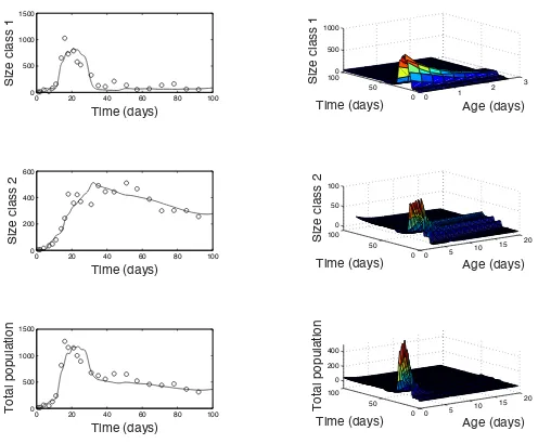
Figure 3: Density-dependent SPM fit to data for replicate 1. Daphnids separated into size class one (top), size class 2 (middle) and total population (bottom). On the left, the total number of daphnids in each size class per day, on the right a surface representing age, time and population number.

4.2 SPM Parameter Estimation and Uncertainty

Figure 3 displays the density-dependent SPM fit to the data for replicate 1 with optimized parameters. The fits are broken up into each size class as well as the total population. On the left side are the total population numbers at each day for each class and on the right is a surface representing dynamics of age, time, and population number. The data is shown with open circles and the model fit in a solid black line. The model solution for replicate one appears to fit each size class as well as the total population.

A similar plot for replicate 2 is shown in Figure 4. We can see that in replicate 2, the optimized fit does not appear as accurate, especially with size class one during the early portion of the simulation. During this time, we can see that there is a sharp increase in size class one, which is even higher than the similar increase in replicate 1. Size class two, however, does appear to have an accurate fit.

(11)

0 1 2

3 4

0 50 1000 500 1000

Size class 1

0 5 10

15 20

0 50 100

Size class 2

0 20 40 60 80 100

0 500 1000 1500

Time (days)

Size class 1

0 20 40 60 80 100

0 100 200 300 400 500

Time (days)

Size class 2

0 20 40 60 80 100

0 500 1000 1500 2000

Time (days)

Total population 0 5

10 15 20

0 50 100

0 200 400

Total population

Figure 4: Density-dependent SPM fit to data for replicate 2. Daphnids separated into size class one (top), size class 2 (middle) and total population (bottom). On the left, the total number of daphnids in each size class per day, on the right a surface representing age, time and population number.

The standard errors are relatively small. Although the optimized parameterq for replicate 2 is outside the range of the 95% confidence interval generated in replicate 1, the optimized parameterq for replicate 1 is inside the range of the 95% confidence interval generated in replicate 2. The parameter c1 for each replicate remains outside of the others’ confidence

interval. Additional replicates would be useful in determining which set of parameters is more descriptive of population dynamics.

(12)

Parameter Estimate (Rep1) 95% CI (Rep1) SE (Rep1)

q 105.0066 ( 78.0305 , 131.9826) 13.8339

c1 0.0142 ( 0.0128, 0.0156 ) 7.0377e-4

q 145.2262 ( 92.1917 , 198.2607 ) 27.1972

c1 0.0191 ( 0.0170 , 0.0212 ) 0.0011

Table 3: Optimal parameters, confidence intervals, and standard errors for replicates 1 and 2.

0 50 100

−300 −200 −100 0 100 Time (days)

0 500 1000

−300 −200 −100 0 100 Model

0 50 100

−200 −100 0 100 200 Time (days)

0 200 400 600

−200 −100 0 100 200 Model

0 50 100

−300 −200 −100 0 100 Time (days)

0 500 1000

−300 −200 −100 0 100 Model

0 50 100

−100 −50 0 50 100 150 Time (days)

0 100 200 300 400 −100 −50 0 50 100 150 Model

Figure 5: Residual plots for replicate one (right) and replicate two (left) for each class size and against time and model value. Residuals appear random, implying the statistical error model is sufficient.

4.3 Sensitivity Analysis

We perform a local sensitivity analysis for the parameters for each replicate and each size class as well as the full population size. Figure 6 displays the results of this sensitivity analysis. Replicate one is shown in black and replicate two is shown in red. The vertical dashed line is the time at which the daphnia population reaches it’s peak during the experiments and occurs at the same time for both replicates. Sensitivities were calculated using the complex-step method [33] and were corroborated with the finite-differencing.

(13)

0 10 20 30 40 50 60 70 80 90 100 0

0.5 1 1.5 2

Size class 1

Normalized sensitivity

q

0 10 20 30 40 50 60 70 80 90 100 −0.5

0 0.5 1

Size class 2

0 10 20 30 40 50 60 70 80 90 100 0

0.2 0.4 0.6 0.8 1

Time

Total Population

0 10 20 30 40 50 60 70 80 90 100 −1

−0.5 0 0.5 1

c

1

0 10 20 30 40 50 60 70 80 90 100 −1.5

−1 −0.5 0

0 10 20 30 40 50 60 70 80 90 100 −1

−0.8 −0.6 −0.4 −0.2 0

Time

(14)

The right panels in Figure 6 show the sensitivity ofc1. The parameter c1 is the linear

relationship between density-dependent mortality and biomass,M(t) (equation (4)). For the total population size, we see that increasingc1 results in lower population levels, which

is sensible, as it increases the density-dependent death rate. However, the dynamics are very different depending on whether we are looking at size class 1 or size class 2. For size class 1, increasingc1 results in lower size class 1 populations for approximately the first 30

days of the experiment, after which increasingc1 results in higher size class 1 populations.

This is also somewhat intuitive since populations of size class 1s are very large in the first 30 days, meaning that the biomass is quite large, which increases the death rate. However, in later times, population levels are low, which means that increasingc1may not be enough

to overcome the small values ofM(t).

In general, the sensitivities for replicate 1 and replicate 2 have similar overall shapes, although replicate 2 tends to show more oscillatory behavior.

4.4 Model Comparison

In addition to our current model, we also proposed a slight variation in the dependent death term, changing the linear relationship between biomass and density-dependent death rate to a hill function. This results in changing equation (4) to

µdep(a, M(t)) = 1 +

c1M(t)h1

ch1

2 +M(t)h1

ch2

3

ch2

3 +ah2

. (22)

where c2 and h1 are optimized along withq and c1. This change allows further range of

flexibility in how the density-dependent death rate depends on the total biomass,M(t). We perform the same optimization as outlined above including calculating the cross-validation score, optimizing parameters, and determining confidence intervals. We obtain a similar cross-validation, withτ = 16 days being the optimalτ, maximizing equation (21). The resulting optimal parameter fits are displayed in Figures 7 and 8 for replicates 1 and 2, respectively.

By eye, the fits to data for the linear density-dependent death rate and the hill function density-dependent death rate appear similar. The optimized parameters for the hill func-tion density-dependent death rate are given in Table 4. We see that our estimates for q

are similar to the 2-parameter model. However, when we examine the confidence intervals and the standard errors, we can see a large decrease in performance from the 2-parameter model. Three of the four parameters for replicate one have confidence intervals which contain negative values, which is not biologically feasible. For replicate two, there are two parameters which also contain negative values.

(15)

0 1

2 3

0 50 1000 500 1000

Size class 1

0 5

10 15 20

0 50 100

Size class 2

0 20 40 60 80 100

0 500 1000 1500

Time (days)

Size class 1

0 20 40 60 80 100

0 200 400 600

Time (days)

Size class 2

0 20 40 60 80 100

0 500 1000 1500

Time (days)

15 20 0

50 100

0 200 400

Age (days)

Group1 tau16

Time (days)Total population

Figure 7: Density-dependent SPM fit to data for replicate 1 using density-dependent death rate given by equation (22). Daphnids separated into size class one (top), size class 2 (middle) and total population (bottom). On the left, the total number of daphnids in each size class per day, on the right a surface representing age, time and population number.

q 94.4182 ( 16.9937 , 171.8428 ) 39.7049

c1 42.5335 ( -382.2441 , 467.3111 ) 217.8347

c2 1533.9 ( -14107 , 17175 ) 8021.2

h1 1.4986 ( -1.4233 , 4.4206 ) 1.4984

q 154.2988 ( -62.2655 , 370.8632 ) 111.0586

c1 16.5795 ( 13.7050 , 19.4541 ) 1.4741

c2 452.3498 ( 356.5672 , 548.1324 ) 49.1193

h1 18.6978 ( -33.2882 , 70.6837 ) 26.6595

Table 4: Optimal parameters, confidence intervals, and standard errors for the 4-parameter model. In this case, many confidence intervals include negative values which is not biolog-ically feasible.

(16)

0 1 2 3 0 50 1000 500 1000 Age (days) Time (days)

Size class 1

0 5

10 15 20 0 50 100 0 50 100 Age (days) Time (days)

Size class 2

0 20 40 60 80 100

0 500 1000 1500

Time (days)

Size class 1

0 20 40 60 80 100

0 100 200 300 400 500 Time (days)

Size class 2

0 20 40 60 80 100

0 500 1000 1500 2000 Time (days)

15 20 0 50 100 0 200 400 Age (days) Time (days)Total population

Figure 8: Density-dependent SPM fit to data for replicate 2 using density-dependent death rate given by equation (22). Daphnids separated into size class one (top), size class 2 (middle) and total population (bottom). On the left, the total number of daphnids in each size class per day, on the right a surface representing age, time and population number.

accurately estimated.

The small standard errors suggest that the 2-parameter model may be more advanta-geous to use, however, we want to ensure that by simplifying the model, we are not losing our ability to describe the dynamics. In order to compare the two models, we turn to the Akaike Information Criteria (AIC) score [3]. The AIC score is an unbiased measure of how well a model fits data. The AIC score is given by:

AIC =N bln

RSS N b

+N b(1 + ln(2π)) + 2(p+ 1) (23)

where N represents the number of data observations, b represents the number of observ-ables, in this case size class 1 (juveniles) and size class 2 (adults), p is the number of parameters being estimated, and RSS is the residual sum of squares. A lower AIC score implies higher accuracy.

(17)

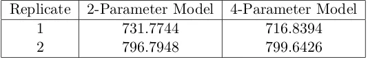
Replicate 2-Parameter Model 4-Parameter Model

1 731.7744 716.8394

2 796.7948 799.6426

Table 5: AICC scores for the 2-parameter model and 4-parameter model for the two

repli-cates.

by:

AICC =AIC+ 2

˜

p(b+p+ 1)

N−(b+p+ 1) (24)

where ˜prepresents the total number of free parameters in the mathematical and statistical models. In our case ˜p=p+ 2 since we estimate σ₀2_i in our statistical error model.

The resulting AICC scores for replicates 1 and 2 for the 2-parameter and 4-parameter

model are given in Table 5. The AICC scores for replicate 1 show that there is slight

improvement using the 4-parameter model. However, for replicate 2, the 2-parameter model has a slightly lower AICC score. We are interested in determining whether there

really is improvement in one model versus the other. To do this, we can calculate the probability of the correct model [37] using Akaike weights [15].

In order to compute the Akaike weights, we need to determine the difference between the best AICC score:

∆i(AICC) =AICCi−minAICC (25)

The Akaike weights are computed using this measure of AICC differences as:

wi(AICC) =

exp−1₂∆i(AICC)

PK

k=1exp

−1

2∆k(AICC)

(26)

Note that PK

k=1wk(AICC) = 1, since the Akaike weights represent the probability that

model i is the correct model. Therefore, the model with the higher Akaike weight is considered to be the better model [37]. We calculate the wi(AICC) for replicates 1 and

two for the 2-parameter and 4-parameter models. For replicate 1, the Akaike weights are 0.0006 and 0.9994 for the 2-parameter and 4-parameter models, respectively. This suggests that the 4-parameter model outperforms the 2-parameter model. However, for replicate 2, the Akaike weights are 0.8059 and 0.1941 for the 2-parameter and 4-parameter models. This suggests that the 2-parameter model outperforms the 4-parameter model.

(18)

5 Discussion and Conclusions

We proposed a continuously structured population model that included both density-dependent and density-indensity-dependent growth, fecundity, and mortality for Daphnia magna

populations. The model that we proposed was used to fit longitudinal experimental data of population dynamics of Daphnia magna.

The model was fit to data using a generalized least-squares framework. We also gener-ated parameter estimates and their associgener-ated confidence intervals. For the two parameters that were estimated, we performed local sensitivity analysis to further understand the ef-fect of changing their values. Additionally, we proposed a slightly more complicated model with two more parameters and showed that our two-parameter model was not inferior at fitting the data, according to the Akaike Information Criteria score. Our two-parameter model had sensible confidence intervals around parameters (non-negative) while the four-parameter model included negative values in the confidence intervals. We learned that, for our data, the density-dependent death rates (equation (4) for the 2-parameter model and equation (22) for the 4-parameter model) should be linear with respect to total biomass,

M(t).

Data collection for this experiment was labor-intensive and we hypothesized whether we could have generated as good a fit with less frequent data collection. To this end, we ran some initial simulations reducing the total number of data points to examine which points were most important to determining parameter estimates. Initial results suggest that such frequent data collection is unnecessary but that consistent collection of data may be more important. We examine the standard errors (SEs) for weekday data collections (M-F every week), 3x a week collection (M/W/F every week), 2x a week collection (M/F or T/T every week) and once weekly collection. The SEs for all of these alternative schedules, with the exception of once weekly, were lower than the SE obtained with our collection schedule (M/W/F for first 3 weeks, thereafter weekly), even though, in some cases, the total number of data points collected were similar. The once-weekly collection SE was on par with the SE generated by our collection schedule for replicate 1 and slightly larger SE value for replicate 2.

The above results suggest that data collection timing is extremely important to the success of our modeling efforts. In order to shrink our standard errors, experimental design will emerge as a powerful tool to dictate experimental efforts. We plan to fully investigate optimal design of experiments in a subsequent paper.

Acknowledgements

(19)

Collection Schedule Replicate 1 Replicate 1 Replicate 2 Replicate 2 (# time points) SE q(105.0066) SE c1(0.0142) SE q(145.2262) SE c1(0.0191)

M-F Weekly (67) 6.6426 4.0209e-04 13.7059 6.0155e-04

M/W/F Weekly (40) 8.5031 51848e-04 17.7146 7.7890e-04

Tu/Th Weekly (27) 10.6405 6.3693e-04 21.6359 9.4698e-04

M/F Weekly (26) 10.6868 6.3771e-04 22.0443 9.5791e-04

Weekly (14) 14.4262 9.0486e-04 30.0295 0.0014

Our Schedule (25) 13.8339 7.0377e-4 27.1972 0.0011

Table 6: SE values for various data collection schedules for Replicate 1 and Replicate 2 for the optimized parameters.

References

[1] Adoteye, K., Banks, H., Flores, K. B., and LeBlanc, G. A. (2015a). Estimation of time-varying mortality rates using continuous models for daphnia magna. Applied

Math-ematics Letters, 44:12–16.

[2] Adoteye, K., Banks, H. T., Cross, K., Eytcheson, S., Flores, K. B., LeBlanc, G. A., Nguyen, T., Ross, C., Smith, E., Stemkovski, M., et al. (2015b). Statistical validation of structured population models for daphnia magna. Mathematical Biosciences, 266:73–84.

[3] Akaike, H. (1974). A new look at the statistical model identification.IEEE Transactions

on Automatic Control, 19(6):716–723.

[4] Ankley, G. T., Bennett, R. S., Erickson, R. J., Hoff, D. J., Hornung, M. W., Johnson, R. D., Mount, D. R., Nichols, J. W., Russom, C. L., Schmieder, P. K., et al. (2010). Adverse outcome pathways: a conceptual framework to support ecotoxicology research and risk assessment. Environmental Toxicology and Chemistry, 29(3):730–741.

[5] Baldwin, W. S. and Leblanc, G. A. (1994). Identification of multiple steroid hydroxy-lases in daphnia magna and their modulation by xenobiotics. Environmental Toxicology

and Chemistry, 13(7):1013–1021.

[6] Banks, H., Banks, J. E., Dick, L. K., and Stark, J. D. (2007). Estimation of dynamic rate parameters in insect populations undergoing sublethal exposure to pesticides. Bulletin

of Mathematical Biology, 69(7):2139–2180.

(20)

[8] Banks, H., Davis, J. L., Ernstberger, S. L., Hu, S., Artimovich, E., and Dhar, A. K. (2009). Experimental design and estimation of growth rate distributions in size-structured shrimp populations. Inverse Problems, 25(9):095003.

[9] Banks, H. T., Catenacci, J., and Hu, S. (2015). Use of difference-based methods to explore statistical and mathematical model discrepancy in inverse problems. Journal of

Inverse and Ill-posed Problems, 24(4):413–433.

[10] Banks, H. T., Everett, R. A., Hu, N. M., and Tran, H. T. (2016) Mathematical and statistical model misspecifications in modeling immune response in renal transplant recipients. Technical Report CRSC-TR16-14, Center for Research in Scientific Compu-tation, N C State University, Raleigh, NC, December. Inverse Problems in Science and

Engineering, submitted.

[11] Banks, H. T., Hu, S., and Thompson, W. C. (2014). Modeling and Inverse Problems

in the Presence of Uncertainty. CRC Press, Boca Raton.

[12] Banks, H. T. and Tran, H. (2009). Mathematical and Experimental Modeling of

Phys-ical and BiologPhys-ical Processes. CRC Press, Boca Raton.

[13] Banks, J. E., Dick, L., Banks, H., and Stark, J. D. (2008). Time-varying vital rates in ecotoxicology: selective pesticides and aphid population dynamics. Ecological Modelling, 210(1):155–160.

[14] Baraldi, R., Cross, K., McChesney, C., Poag, L., Thorpe, E., Flores, K. B., and Banks, H. (2014). Uncertainty quantification for a model of HIV-1 patient response to antiretroviral therapy interruptions. Technical Report CRSC-TR13-13, Center for Research in Scientific Computation, N C State University, Raleigh, NC, October, 2013.

In2014 American Control Conference, pages 2753–2758. IEEE.

[15] Burnham, K. P. and Anderson, D. R. (2002)Model Selection and Multimodel Inference:

A Practical Information-theoretic Approach. Springer, New York.

[16] Caswell, H. (1989). Matrix Population Models: Construction, Analysis, and

Interpre-tation Sinauer Associates, Sunderland, MA.

[17] Caswell, H. (2005). (ed.) Food Webs: From Connectivity to Energetics Advances in Ecological Research 36. Elsevier Academic Press, San Diego, California.

[18] Council, N. R. (2013). Assessing Risks to Endangered and Threatened Species from

Pesticides. The National Academies Press, Washington, DC.

(21)

[20] Diekmann, O., Gyllenberg, M., and Metz, J. (2007). Physiologically Structured

Pop-ulation Models: Towards a General Mathematical Theory. Springer-Verlag, Berlin

Hei-delberg.

[21] El-Doma, M. (2011). Stability analysis of a size-structured population dynamics model of daphnia. International Journal of Pure and Applied Mathematics, 70(2):189–209.

[22] El-Doma, M. (2012). A size-structured population dynamics model of daphnia.Applied

Mathematics Letters, 25(7):1041–1044.

[23] Ellner, S. P., Childs, D. Z., and Rees, M. (2016). Data-driven Modelling of Structured

Populations: A Practical Guide to the Integral Projection Model.Springer-Verlag, Berlin.

[24] Ellner, S. P. and Guckenheimer, J. (2011). Dynamic Models in Biology. Princeton University Press. Princeton, NJ.

[25] Erickson, R. A., Cox, S. B., Oates, J. L., Anderson, T. A., Salice, C. J., and Long, K. R. (2014). A daphnia population model that considers pesticide exposure and demographic stochasticity. Ecological Modelling, 275:37–47.

[26] Farkas, J. Z. and Hagen, T. (2007). Linear stability and positivity results for a gener-alized size-structured daphnia model with inflow. Applicable Analysis, 86(9):1087–1103.

[27] Finkel, D. E. and Kelley, C. T. Convergence analysis of the direct algorithm.

Opti-mization Online, 14(2):1–10.

[28] Hanson, N. and Stark, J. D. (2011). A comparison of simple and complex population models to reduce uncertainty in ecological risk assessments of chemicals: example with three species of daphnia. Ecotoxicology, 20(6):1268–1276.

[29] Keyfitz, N. and H. Caswell, H. (2005). Applied Mathematical Demography, Third

edition Springer-Verlag, New York, NY

[30] Kramer, V. J., Etterson, M. A., Hecker, M., Murphy, C. A., Roesijadi, G., Spade, D. J., Spromberg, J. A., Wang, M., and Ankley, G. T. (2011). Adverse outcome path-ways and ecological risk assessment: Bridging to population-level effects. Environmental

Toxicology and Chemistry, 30(1):64–76.

[31] LeBlanc, G. A., Wang, Y. H., Holmes, C. N., Kwon, G., and Medlock, E. K. (2013). A transgenerational endocrine signaling pathway in crustacea. PloS One, 8(4):e61715.

[32] Leslie, P. H. (1945). On the use of matrices in certain population mathematics.

Biometrika, 33(3):183–212.

(22)

[34] Rider, C. V. and LeBlanc, G. A. (2005). An integrated addition and interaction model for assessing toxicity of chemical mixtures. Toxicological Sciences, 87(2):520–528.

[35] Shampine, L. (2005). Solving hyperbolic pdes in matlab. Applied Numerical Analysis

& Computational Mathematics, 2(3):346–358.

[36] Sinko, J. W. and Streifer, W. (1967). A new model for age-size structure of a popu-lation. Ecology, 48(6):910–918.

[37] Wagenmakers, E. and Farrell, S. (2004) AIC model selection using Akaike weights.

Psychonomic Bulletin & Review, 11(1):192–196.

[38] Wang, H. Y., Olmstead, A. W., Li, H., and LeBlanc, G. A. (2005). The screening of chemicals for juvenoid-related endocrine activity using the water flea daphnia magna.

Aquatic Toxicology, 74(3):193–204.

[39] Wang, Y. H., Kwon, G., Li, H., and LeBlanc, G. A. (2011). Tributyltin synergizes with 20-hydroxyecdysone to produce endocrine toxicity. Toxicological Sciences, 123(1):71–79.