Small Satellite Cloud Detection Based On Deep Learning and Image Compression

Small Satellite Cloud Detection Based On Deep

Learning and Image Compression

Zhaoxiang Zhang1,, Akira IWASAKI2,Guodong Xu1,and Jianing Song1,

1 _{Harbin Institute of Technology, Harbin, China;}

2 _{University of Tokyo, Tokyo, Japan}

Abstract:An effective on-board cloud detection method in small satellites would greatly improve the downlink data transmission efficiency and reduce the memory cost. In this paper, an ensemble method combining a lightweight U-Net with wavelet image compression is proposed and evaluated. The red, green, blue and infrared waveband images from Landsat-8 dataset are trained and tested to estimate the performance of proposed method. The LeGall-5/3 wavelet transform is applied on the dataset to accelerate the neural network and improve the feasibility of on-board implement. The experiment results illustrate that the overall accuracy of the proposed model achieves 97.45% by utilizing only four bands. Tests on low coefficients of compressed dataset have shown that the overall accuracy of the proposed method is still higher than 95%, while its inference speed is accelerated to 0.055 second per million pixels and maximum memory cost reduces to 2Mb. By taking advantage of mature image compression system in small satellites, the proposed method provides a good possibility of on-board cloud detection based on deep learning.

Keywords:Cloud detection; Deep learning; Image Compression.

0. Introduction

The global cloud covers is approximately 66% over land surfaces of the Earth, and it often appears and covers objects on the surface in remote sensing images, which makes much difficulty in image analysis tasks and object detection missions [1]. Good cloud detection algorithms are always necessary especially before the implement of segmentation and object detection methods.

What’s more, with the trend of satellite missions towards lower cost and wide coverage, the on-board cloud detection draws great attention in the research area [2], [3], [4], [5]. Since the convolutional neural networks (CNN) have demonstrated excellent performance in various visual recognition problems such as image classification [6], [7], CNN would provide better possibility of accurate on-board cloud detection in small satellites. Besides, as for the smaller and lighter satellites aiming at lauch cost reduction, which requires smaller and low-cost optical payload, the spectral information is limited for image processing. In general, small satellite images are composed of at most four wavebands including red, green, blue and infrared, thus, most of existing state-of-art threshold-based methods, such as FMask [8], ACCA [9] and MSScvm [10], could not demonstrate satisfactory performance without extra information like far infrared data or atmosphere temperature.

Since the cloud detection tasks applied on the satellite platforms are more constrained by the hardware limits (such as memory storage and power restriction) than the classification algorithms, and the consuming time of on-board deep learning would be intolerable, satellite image compression systems should be considered to concentrate image features and accelerate the algorithms. In most satellites, the images would be transmitted directly to the ground station after compression, and uncompressed data is hard to adopted in small satellites for classification. On the other hands, the low-frequency coefficients of the compressed images show great potential on image detection tasks such as face recognition [11].

This paper proposed a lightweight deep neural networks based on U-Net, and obtained better overall accuracy while reaches to the state-of-art inference speed by applying the LeGall-5/3 wavelet transform [12] on the dataset. The SPARCS dataset based Landsat-8 [13] is utilized here and the

Overall Accuracy on test data achieves 97.43%. Comparing with the state-of-art method F-mask and SPARCS [13], which achieve 99.1% and 98.1% on Overall Accuracy separately by utilizing full 11 bands including Cirrus Band and Thermal Infrared Band, the proposed method shows competitive performance only taking advantage of texture and geometric features from RGB and Infrared Bands. After image compression is applied, the overall accuracy comes to 95.2% on the level-4 compressed images, where the size of the compressed image narrows down to 16×16, and the inference speed of the proposed method reduces from 7.23sto 0.055s, along with the maximum memory cost reducing from 162.2Mbinto 2.07Mb. Therefore, it provides a great possibility of implement of the on-board deep learning algorithms to solve the high-resolution remote sensing image classification problems, especially when rough cloud fraction needs to be calculated before image transmission. A comparison with different algorithms including machine learning based method and threshold-based method on the same dataset proves the validity and efficiency of our algorithm.

1. Background

In recent years, scholars have undertaken a great deal of research into cloud and cloud shadow detection for different types of remote sensing data and several popular algorithms are proposed. Since abundant spatial information is contained in the four waveband images, and since human classifiers can almost always visually identify clouds within a scene, spatial information should be sufficient for discrimination. The convolutional neural networks (CNN) have been proven to gather and utilize image spatial information effectively, and it has shown excellent performance in various visual recognition problems such as image classification, object detection, semantic classification and action recognition.

Methods based on deep learning algorithms have been introduced in this area in very recent years [14], [15]. Sholar [14] illustrates a lightweight constitutional neural network for cloud detection. Shi, etc. [16] proposed a nerual network combined with super-pixel pre-classification method to achieve a rough coud mask. While Xie, etc. [17] demonstrates a segmentation method combined with two neural net works with different input size. However, most of the existing deep learning methods combine with super-pixel segmentation method, which utilize super-pixel areas as input patches and obtain single output for every patch. Therefore, existing methods could not obtain the pixel-wise detection accuracy and is not able to achieve good classification performance on compressed images with small size like 16×16. Therefore, some new deep learning networks designed for semantic segmentation such as U-Net should be introduced here to achieve better accuracy on compressed dataset.

Several works have also taken efforts on other methods. In [18] Chie, etc. demonstrated a cloud classification method on low-resolution images based on texton random forest, which explores the potential possibility of on-board image processing in simple tasks. Weng, etc. [19] introduced deep extreme learning machine to classify the images from HJ-1A/1B satellite and compute the cloud cover fraction. And Bartos, etc. [20] illustrated the performance of segNet model combined with hard negative mining method on cloud detection mission. A threshold-based method in [21] combined the threshold segmentation with geometric feature and texture feature to detect cloud of GaoFen-1 images.

U-Net model was proposed by Olaf Ronneberger in 2015 [22]. By combining the high-resolution layers with decoded low resolution images, and utilizing upsampling operators to reach the pixel-wise result, U-Net framework has shown great performance on large biomedical images and won the ISBI cell tracking challenge 2015. Thus, it shows great potential on pixel-wise classification of remote sensing dataset.

2. Method

2.1. Data set up

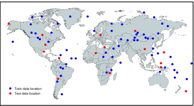
Figure 1.WRS2 path/row data location of imagery utilized for training and test

are several reasons that we select the SPARCS dataset: 1, according to article [13], the pixel-wise cloud masks by the SPARCS dataset is acquired by 11 bands of Landsat-8 datasets and the groundtruth accuracy is high enough considering that we only use four bands for training and testing; 2, different circumstances including large thin cloud area, cloud over ocean, cloud over ice and snow are contained in the dataset, which would make the proposed method more persuasive. 3, the classification results in [13] by utilizing 11 bands provide a good comparison with the proposed method.

The dataset was originally created by M. Joseph Hughes, Oregon State University, from Landsat 8 Operational Land Imager (OLI) Level-1B scenes. The purpose of the data was to validate cloud and cloud shadow masking derived from the Spatial Procedures for Automated Removal of Cloud and Shadow (SPARCS) algorithm. SPARCS data has seven manually labeled classes, including cloud, shadow, flooded, ice/snow, water, shadow over water, and land. Each mask is a 1000×1000 pixel subset of an original Landsat 8 OLI/TIRS Level-1 scene with 11 spectral bands. In this paper, only band 2, 3, 4, 5, which is Red, Blue, Green and infrared bands are utilized for training and testing, and the classes are reclassified as two classes including cloud and non-cloud.

According to the reference [13], the overall 80 images are separated into two groups: 80% as training set and 20% as test set. We carefully pick twelve representative scenes as test images to make sure that every class is included and each class ratio in two groups keep approximately the same. Beside, the geographical location is also considered, and the training and test dataset varies from different hemispheres and latitudes, which is shown in Fig.1. What’s more, considering the limitation of GPU memory, the original image is divided into sub-images with 300×300 size and becomes the input data for the proposed model.

2.2. Neural Network Classification

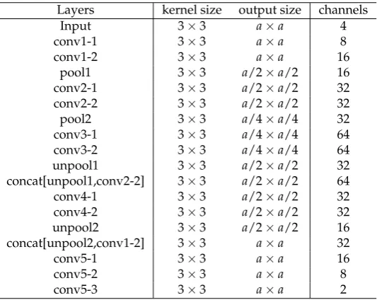
Table 1.Architecture of proposed lightweight U-Net: L-unet;adepends on the input image size

Layers kernel size output size channels

Input 3×3 a×a 4

conv1-1 3×3 a×a 8

conv1-2 3×3 a×a 16

pool1 3×3 a/2×a/2 16

conv2-1 3×3 a/2×a/2 32

conv2-2 3×3 a/2×a/2 32

pool2 3×3 a/4×a/4 32

conv3-1 3×3 a/4×a/4 64

conv3-2 3×3 a/4×a/4 64

unpool1 3×3 a/2×a/2 32

concat[unpool1,conv2-2] 3×3 a/2×a/2 64

conv4-1 3×3 a/2×a/2 32

conv4-2 3×3 a/2×a/2 32

unpool2 3×3 a/2×a/2 16

concat[unpool2,conv1-2] 3×3 a×a 32

conv5-1 3×3 a×a 16

conv5-2 3×3 a×a 8

conv5-3 3×3 a×a 2

Table 2.Architecture of the L-decov.adepends on the input image size

Layers kernel size output size channels

Input 3×3 a×a 4

conv1 3×3 a×a 8

conv2 3×3 a×a 16

fc3 1×1 a×a 32

fc4 1×1 a×a 32

deconv2 3×3 a×a 16

deconv1 3×3 a×a 8

output 1×1 a×a 2

adopted between layers, and Cross-entropy cost function and Adam optimizer are utilized here to train the network. The architecture of the proposed lightweight networks (hereinafter referred to as L-unet) is illustrated in Table.1. The output size a in Table.1depends on the size of the input data. For example,awould change from 300 to 150 when the original dataset is compressed in one level.

Considering that another popular architecture for pixelwise segmentation in deep learning community is deconvolutional layer which was first proposed by Hyeonwoo Noh in 2015. And in order to achieve better comparison with proposed network, another lightweight model (hereinafter referred to as L-decov) based on [14] is developed, The network with only 7 layers is developed based on Segnet [23] and DeconvNet [24]. It shares simliar deconvolution layers with DeconvNet. The deconvolution layers is the transpose convolution layer which is a reverse convolution turning convoluted images into their original size. It would help the neural network achieve the pixel-wise detection precision. Several slight changes are applied for the original network. The input size is adjusted according to the sample size of the training data. Besides, channels of every layer in L-decov network are reduced compared with the original network. We carefully select the channels of each network to make sure that their inference speed and memory cost is close on same dataset in same hardware environment. Therefore, a better comparison could be achieved. The architecture of L-decov is illustrated in Table.2. Similarly, the output sizeawould be adjusted as the input size changes.

LL ↓2 ↓2 H0 H1 LL LH H0 H1 HL HH H0 H1 Image corres. to resolution. level i-1 Image corres. to res. level i

Detail Images at resolution level i

(a) One Filter Stage in 2D DWT

1HL 1LH 1HH 2HH 2LH 3HL 3LL 3LH 3HH 2HL

(b) Structure of wavelet decomposition

Figure 2.Discrete wavelet decomposition

2.3. Image compression

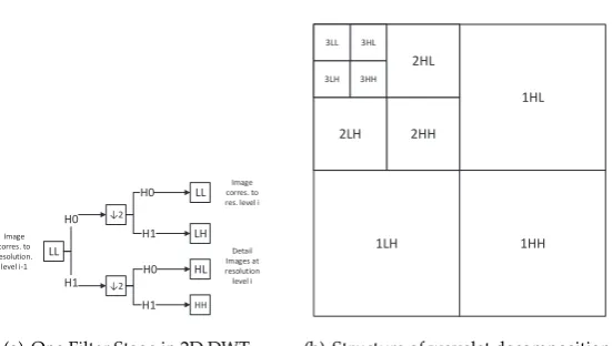
Since proposed neural network would be time-consuming for on-board satellite applications, the compressed images would be considered as the input data. Image compression technology is required to deal with the large volume of data produced by multi-spectral sensors [25]. Discrete Wavelet Transform (DWT) algorithms have been utilized in most of the earth observation satellites during the last few decades. [26]. In a typical data compression system, the first step is the two dimensional DWT based forward transformation, separating images into high-frequency and low-frequency part, in order to concentrate the most essential signal into the few low frequency parts. The DWT algorithm is employed in several systems like JPFG2000 [27], Embedded Zero tree Wavelet algorithm (EZW) [28], or Set Partitioning In Hierarchical Trees (SPIHT) [29]. The on-board compression theory has been developed for decades and mature compression systems have been applied in satellites successfully.

The theory of the two dimensional DWT method has been throughly studied and widely discussed in recent years. Plenty of wavelets, such as Haar wavelet [30], Symmetric wavelet [31], and LeGall-5/3 Wavelet, [32] have been introduced into the image compression system. For the two-dimensional images, the wavelets would be applied three times that scan the image details in horizontal, vertical and diagonal directions. It could be represented as a four channel perfect reconstruction filter bank as shown in Fig.2(a). Then this process could be repeated on the low low (LL) band utilizing the second stage of identical filter bank. Thus, a typical two-dimensional DWT, utilized in image compression, generates the hierarchical structure shown in Fig.2(b).

Table 3. Classification results of different algorithms on 16 test dataset, NN is the neural network developed based on [13]

Algorithms Overall Accuracy Recall F1score Proposed L-unet 0.9745 0.9169 0.9449

L-decov 0.9646 0.8280 0.8904

Adaboost 0.9138 0.7077 0.7977

Random Forest 0.9266 0.7225 0.8119

Neural Network 0.873 0.698 0.776

SVM 0.902 0.684 0.7780

3. Results and Discussion

3.1. Classification results

We trained the proposed models in last section and several algorithms are introduced to compare with our method. A classical random forest method with iteration parameters setting to 20 is applied to the training data, and the result of test data is illustrated. Besides, an Adaboost method is also implemented, while the iteration parameter is also set to 20. And a SVM method with radial basis function kernel(RBF) is introduced and evaluated. According to [13], a pixelwise neural network with a hidden layer of 30 nodes are developed and evaluated. Considering about the lack of spatial information after image compression, the post processing steps developed in [13] is not introduced here. The input size of the neural network is changed since only four bands of the dataset are utilized here while the whole 11 band images are required in [13]. The algorithms are implemented based on the scikit-learn library in Python environment. Four waveband information for each pixel is reshaped as feature vectors to train and test these models. The selection of training and test dataset keeps the same as the two deep learning networks mentioned in last section.

We choose Overall Accuracy, Recall andF1scoreto evaluate the performance of the algorithms.

TheF1scoreis the harmonic mean of Accuracy and Recall:

F1score=

2×Accuracy×Recall

Accuracy+Recall (1)

The cloud detection results of the 16 test images are illustrated in Table. 3. The results show that the proposed method, L-unet expresses the best performance in all indicators on the test dataset. Compared with overall accuracy, the Recall score decreases for all algorithms, while the proposed method still has a obviously good performance, which shows strong capability on cloud detection. The Neural Network developed based on [13] could not achieve satisfactory accuracy because of lack of spectral information especially band 6, band 9, band 10, and band 11. As for the Random Forest, Adaboost and Svm methods which could not take advantage of texture features from neighboring pixels, the overall accuracy and recall is not good enough compared with the two convolutional networks. To make effective comparison without losing impartiality, the segmentation results obtained from the best four methods including L-unet, L-decov, Random Forest and Adaboost are illustrated and further evaluated on compressed dataset.

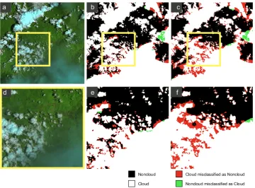
Figure 3. Image classification of a sub-scene from Kyauktazi, South Myanmar (WRS2 path/row 133/49), acquired on 21 May 2014. (a): False color image; (b): Results obtained by proposed method; (c): by L-decov; (d): by Adaboost; (e): by Random Forest

good performance on heavy cloud while L-decov netowrk mis-classified the land between the thin cloud, as illustrated in the yellow rectangle of Fig. 4. The reason that L-unet network has better classification accuracy on thin cloud is, the high resolution layers are participated in the training process in the decoding parts of the networks, which provides a larger vision for the training model. That is, the texture and geometric characteristics are well analyzed and evaluated to make sure a good performance in borders of different classes.

Fig.5shows the scene from Swiss alps, Switzerland (WRS2 path/row 195/28), which is introduced here to evaluate the performance of the proposed method on ice and snow area. Fig.5(b) illustrates the groundtruth of the image, in which the blue areas represent the ice from the Alps, Fig.5(c) illustrates that the proposed network could well distinguish the ice from the cloud based on its geometric features.

Fig.6shows a sub-scene from Carangas, Bolivia (WRS2 path/row 1/73), which belongs to another Landsat dataset Bimoes [33]. The image is introduced here to illustrate that the proposed method still have better performance on different dataset. The comparison of Fig.6(b) and Fig.6(c) has shown that the bright area between the mountains could be well distinguished from cloud by the proposed method.

To further verify the performance of proposed method, the cloud detection recall of different classes in the test dataset are illustrated in Table.4. The results demonstrate that although L-decov method shows slightly better detection recall in land areas, the proposed L-unet method performs better in most classes, especially in the cloud area. That is, thin cloud areas, cloud over water, and cloud over bright areas would be well distinguished by proposed method.

3.2. Compressed image classification

Figure 4.Image classification of a sub-scene from South Sulawesi, Indonesia (WRS2 path/row 114/62), acquired on 27 February 2014. (a): False color image; (b): Results obtained by proposed method; (c): Results obtained by L-decov; (d): sub scene of (a); (e): sub scene of (b); (f): sub scene of (c)

Figure 5. (a) A sub-scene from Swiss alps, Switzerland (WRS2 path/row 195/28), acquired on 12 February 2014. (b): Groundtruth of image (a); (c): Classification result of image (a)

Table 4.Cloud detection error on different classes

Classes Land Cloud Flood Snow Water Shadow Shadow-over-water

Class ratio 63.67% 20.35% 0.16% 2.82% 7.76% 4.92% 0.32%

Figure 6.(a) A sub-scene from Carangas, Bolivia (WRS2 path/row 1/73), acquired on 03 June 2013; (b): Results obtained by proposed method; (c): Results obtained by L-decov;

Table 5.Overall cloud accuracy with compressed images

Classifiers Level1 Level2 Level3 Level4 Accuracy Decrease Proposed L-unet 0.967 0.964 0.9586 0.952 1.5%

L-decov 0.960 0.9373 0.9373 0.927 3.3%

Adaboost 0.91027 0.90937 0.88726 0.86335 4.7% RandomForest 0.92464 0.91893 0.90752 0.90321 2.1%

its performance. The overall accuracy of different algorithms are shown in Table. 5. The results demonstrated that the proposed method shows the best performance in each level of the compression, and most importantly, the overall accuracy also decreased the least after images compression. Hence, by applying image compression strategy, the proposed model would keep the good performance on cloud fraction accuracy while the computation time and required memory would visibly reduced. In Fig. 7, The compressed image of the sub scene in Puerto Aldea, Chile (WRS2 path/row 1/81) is illustrated. The classification results by L-unet demonstrated that the thin cloud area could still be detected on the compressed image. The results shows that compared with other methods, the proposed L-unet is more robust on the noise introduced by compression operation, and keeps sensitive of thin cloud area on the compressed images.

Table.6demonstrated the inference speed of different algorithms. The speed of the algorithms is verified in python-based environment on the i-7 core computer with 16G RAM. Table.7illustrated the maximum cost of the two networks before and after the image compression. The memory cost is composed of size of neural layers and parameters of weights while memory reuse is not considered. And the data type of the input images is 16 bits integers. The inference speed results and the memory cost results illustrate that the compression process dramatically accelerates proposed neural network and reduces its memory cost. The memory cost of proposed L-unet becomes 2.07Mbafter applying the level-4 images, which is small enough for the ARM-based processors in satellites while considering the power limitation. Besides, the comparison between two networks show that L-decov cost less memory but has larger inference speed, because of the less neural layers and less parameters, along with deconvolutional layers, which would cost more time compared with up-pooling layers.

4. Conclusion and future work

Figure 7.A sub-scene from Puerto Aldea, Chile (WRS2 path/row 1/81), acquired on 13 February 2014; (a): False color image of level-4 compressed images; (b): Result obtained by L-unet wherea=16; (c): Result obtained by L-decov wherea=16

Table 6.Inference speeds for different algorithms

Method Inference Speed (Sec/Mil-Pixels)

L-decov (GPU) 0.218

L-unet (GPU) 0.211

L-decov (no-GPU) 7.62

L-unet (no-GPU) 7.23

L-decov(Level-4, no-GPU) 0.058

L-unet(Level-4, no-GPU) 0.055

Adaboost 2.63

RandomForest 2.5195

Table 7.Maximum memory cost of the two networks

Netwok Input Size Maximum memory cost (Mb)

L-decov 300×300 185.6096

L-unet 300×300 162.1826

Adaboost, and RandomForest are demonstrated to compare with our method. The experiment results illustrated that the proposed model keeps high accuracy after 4-level compression. And the inference speed reaches to 0.055 second/per million pixels, while the maximum memory cost of the network is only 2Mb.

There are still several aspects left for future improvement. To explore the possibility of on-board application for cloud detection, details such as on on board image transformation and algorithms implement would be researched further. The small deep learning neural networks with few layers have become a popular topic since last year. Several improved CNN networks such MobileNet could be verified to further reduce the network size and memory cost. Besides, other datasets such as Landsat-7 dataset should also be used to improve the proposed model.

Acknowledgments

We wish to acknowledge the M. Joseph Hughes in Oregon State University for their open source cloud mask dataset, SPARCS. And we wish to acknowledge the Google LLC for the Google Cloud Platform and its free trial opportunity.

1. Saunders, R.W.; Kriebel, K.T. An improved method for detecting clear sky and cloudy radiances from AVHRR data.International Journal of Remote Sensing1988,9, 123–150.

2. ZHENG, S.; others. Real-Time automatic cloud detection during the process of taking aerial photographs. Spectroscopy and Spectral Analysis2014,34, 1909–1913.

3. Tan, Y.; Qi, J.; Ren, F. Real-time cloud detection in high resolution images using Maximum Response Filter and Principle Component Analysis. Geoscience and Remote Sensing Symposium (IGARSS), 2016 IEEE International. IEEE, 2016, pp. 6537–6540.

4. Shan, N.; Zheng, T.y.; Wang, Z.s. Onboard real-time cloud detection using reconfigurable FPGAs for remote sensing. Geoinformatics, 2009 17th International Conference on. IEEE, 2009, pp. 1–5.

5. Zheng, H.; Li, Z.; Li, Z. Real-time cloud detection that uses data parallel and pipeline. Image and Signal Processing (CISP), 2011 4th International Congress on. IEEE, 2011, Vol. 3, pp. 1652–1655.

6. Krizhevsky, A.; Sutskever, I.; Hinton, G.E. Imagenet classification with deep convolutional neural networks. Advances in neural information processing systems, 2012, pp. 1097–1105.

7. Simonyan, K.; Zisserman, A. Very deep convolutional networks for large-scale image recognition. arXiv preprint arXiv:1409.15562014.

8. Zhu, Z.; Woodcock, C.E. Object-based cloud and cloud shadow detection in Landsat imagery. Remote Sensing of Environment2012,118, 83–94.

9. Irish, R.R.; Barker, J.L.; Goward, S.N.; Arvidson, T. Characterization of the Landsat-7 ETM+ automated cloud-cover assessment (ACCA) algorithm. Photogrammetric engineering & remote sensing 2006, 72, 1179–1188.

10. Yang, Z.; Cohen, W.B.; Braaten, J.D. Automated cloud and cloud shadow identification in Landsat MSS imagery for temperate ecosystems2015.

11. Ramesha, K.; Raja, K. Face recognition system using discrete wavelet transform and fast PCA. InInformation Technology and Mobile Communication; Springer, 2011; pp. 13–18.

12. Bramble, J.M.; Huang, H.; Murphy, M.D. Image data compression.Investigative radiology1988,23, 707–712. 13. Hughes, M.J.; Hayes, D.J. Automated detection of cloud and cloud shadow in single-date Landsat imagery

using neural networks and spatial post-processing. Remote Sensing2014,6, 4907–4926.

14. Sholar, J.M. Lightweight Deconvolutional Neural Networks for Efficient Cloud Identification in Satellite Images.

15. Le Goff, M.; Tourneret, J.Y.; Wendt, H.; Ortner, M.; Spigai, M. Deep Learning for Cloud Detection. 16. Shi, M.; Xie, F.; Zi, Y.; Yin, J. Cloud detection of remote sensing images by deep learning. Geoscience and

17. Xie, F.; Shi, M.; Shi, Z.; Yin, J.; Zhao, D. Multilevel Cloud Detection in Remote Sensing Images Based on Deep Learning. IEEE Journal of Selected Topics in Applied Earth Observations and Remote Sensing2017, 10, 3631–3640.

18. Chien, S.; Doubleday, J.; Thompson, D.; Wagstaff, K.; Bellardo, J.; Francis, C.; Baumgarten, E.; Williams, A.; Yee, E.; Fluitt, D.; others. Onboard autonomy on the Intelligent Payload EXperiment (IPEX) Cubesat mission: A pathfinder for the proposed HyspIRI mission intelligent payload module. Proc 12th International Symposium in Artificial Intelligence, Robotics and Automation in Space, Montreal, Canada, 2014.

19. WENG, L.g.; KONG, W.b.; Min, X. Computing Cloud Cover Fraction in Satellite Images using Deep Extreme Learning Machine.International Journal of Simulation–Systems, Science & Technology2016,17. 20. Bartoš, B.M. Cloud and Shadow Detection in Satellite Imagery2017.

21. Li, Z.; Shen, H.; Li, H.; Xia, G.; Gamba, P.; Zhang, L. Multi-feature combined cloud and cloud shadow detection in GaoFen-1 wide field of view imagery. Remote sensing of environment2017,191, 342–358. 22. Ronneberger, O.; Fischer, P.; Brox, T. U-net: Convolutional networks for biomedical image segmentation.

International Conference on Medical image computing and computer-assisted intervention. Springer, 2015, pp. 234–241.

23. Badrinarayanan, V.; Kendall, A.; Cipolla, R. Segnet: A deep convolutional encoder-decoder architecture for image segmentation. IEEE transactions on pattern analysis and machine intelligence2017,39, 2481–2495. 24. Noh, H.; Hong, S.; Han, B. Learning deconvolution network for semantic segmentation. Proceedings of

the IEEE International Conference on Computer Vision, 2015, pp. 1520–1528.

25. Qian, S.E.; Bergeron, M.; Cunningham, I.; Gagnon, L.; Hollinger, A. Near lossless data compression onboard a hyperspectral satellite.IEEE Transactions on Aerospace and Electronic Systems2006,42.

26. Shihab, H.S.; Shafie, S.; Ramli, A.R.; Ahmad, F. Enhancement of Satellite Image Compression Using a Hybrid (DWT–DCT) Algorithm. Sensing and Imaging2017,18, 30.

27. Rabbani, M.; Joshi, R. An overview of the JPEG 2000 still image compression standard. Signal processing: Image communication2002,17, 3–48.

28. Shapiro, J.M. Embedded image coding using zerotrees of wavelet coefficients. IEEE Transactions on signal processing1993,41, 3445–3462.

29. Said, A.; Pearlman, W.A. A new, fast, and efficient image codec based on set partitioning in hierarchical trees. IEEE Transactions on circuits and systems for video technology1996,6, 243–250.

30. Talukder, K.H.; Harada, K. Haar wavelet based approach for image compression and quality assessment of compressed image. arXiv preprint arXiv:1010.40842010.

31. Palanivelu, L.; Vijayakumar, P. A Hybrid Image Compression Technique using Symmetric Wavelet for Multi-Application Smart Card Application. International Journal of Computer Applications2012,53. 32. Usevitch, B.E. A tutorial on modern lossy wavelet image compression: foundations of JPEG 2000. IEEE

signal processing magazine2001,18, 22–35.