Grohsjean, Alexander (2009): Measurement of the Top Quark Mass in the Dilepton Final State using the Matrix Element Method. Dissertation, LMU München: Fakultät für Physik

Measurement of the Top Quark Mass

in the Dilepton Final State

using the Matrix Element Method

Dissertation

vorgelegt der Fakultät für Physik der

Ludwig-Maximilians-Universität München

von

Alexander Grohsjean

1. Gutachter: Prof. Dr. Otmar Biebel

2. Gutachter: Prof. Dr. Martin Faessler

Zusammenfassung

Das Top-Quark, das 1995 durch die CDF- und DØ-Experimente am Tevatron-Beschleuniger ent-deckt wurde, ist das schwerste aller bisher beobachteten Elementarteilchen. Eine genaue Vermes-sung seiner Masse erlaubt Rückschlüsse auf die Masse des noch unentdeckten Higgs-Bosons und eine Sondierung der Physik jenseits des Standardmodells.

In der vorliegenden Arbeit wird die erste Messung der Top-Quark-Masse mit der Matrix-Element-Methode im dileptonischen Zerfallskanal am DØ-Experiment präsentiert. Nach einer kurzen Beschreibung des Tevatron-Beschleunigers und des DØ-Experiments folgen die Darstel-lung der Rekonstruktion der physikalischen Objekte aus Signalen im Detektor sowie eine de-taillierte Diskussion der Matrix-Element-Methode. Diese basiert auf der Wahrscheinlichkeit, ein bestimmtes Ereignis unter der Annahme der zu messenden Größe, etwa der Top-Quark-Masse, zu beobachten.

Im Vergleich zu bisherigen Messungen im Lepton+Jets-Kanal wird die Methode signifikant verbessert. Die beiden nicht detektierten Neutrinos erfordern ein neues Verfahren zur Rekonstruk-tion der Ereigniskinematik. Die geringe Anzahl an Ereignissen im dileptonischen Kanal macht die Modellierung von zusätzlichen Jets in der Signalwahrscheinlichkeit notwendig. Zur Beschreibung des Hauptuntergrundes von tauonisch zerfallendenZ-Bosonen wird eine neue

Ereigniswahrschein-lichkeit entwickelt.

Die Validierung der erweiterten Matrix-Element-Methode erfolgt mit simulierten Ereignissen auf Generatorniveau. Zur Kalibrierung der Methode werden Monte-Carlo-generierte Ereignisse, die eine vollständige Detektorsimulation durchlaufen haben, verwendet. Die Methode wird auf den verfügbaren Run-II-Datensatz, der zwischen April 2002 und Mai 2008 aufgezeichnet wurde und einer integrierten Luminosität von 2.8 fb−1entspricht, angewendet.

Ins-gesamt werden 107 Ereignisse mit einem Elektron und einem Myon im Endzustand selektiert. Die Anwendung der Matrix-Element-Methode auf diesen Datensatz ergibt eine Top-Quark-Masse von

mRun IIa_top = 170.6_±6.1(stat.)+2.1_−1.5(syst.)GeV

mRun IIb_top = 174.1_±4.4(stat.)+2.5_−1.8(syst.)GeV

mcomb_top = 172.9_±3.6(stat.)_±2.3(syst.)GeV.

Im Anschluss werden die systematischen Unsicherheiten der Messung diskutiert und die Ergebnisse im Rahmen des Standardmodells interpretiert. Da die größte systematische Unsicher-heit durch die absolute Energieskala der Jets bedingt ist, werden Studien für eine gleichzeitige Messung der Top-Quark-Masse und der Energieskala der b-Jets vorgestellt. Die Möglichkeiten,

Abstract

The top quark, discovered in 1995 by the CDF and DØ experiments at the Fermilab Tevatron Collider, is the heaviest known fundamental particle. The precise knowledge of its mass yields important constraints on the mass of the yet-unobserved Higgs boson and allows to probe for physics beyond the Standard Model.

The first measurement of the top quark mass in the dilepton channel with the Matrix Ele-ment method at the DØ experiEle-ment is presented. After a short description of the experiEle-mental environment and the reconstruction chain from hits in the detector to physical objects, a detailed review of the Matrix Element method is given. The Matrix Element method is based on the likelihood to observe a given event under the assumption of the quantity to be measured, e.g. the mass of the top quark.

The method has undergone significant modifications and improvements compared to previous measurements in the lepton+jets channel: the two undetected neutrinos require a new

reconstruc-tion scheme for the four-momenta of the final state particles, the small event sample demands the modeling of additional jets in the signal likelihood, and a new likelihood is designed to account for the main source of background containing tauonicZdecay.

The Matrix Element method is validated on Monte Carlo simulated events at the generator level. For the measurement, calibration curves are derived from events that are run through the full DØ detector simulation. The analysis makes use of the Run II data set recorded between April 2002 and May 2008 corresponding to an integrated luminosity of 2.8 fb−1. A total of 107_tt¯

candidate events with one electron and one muon in the final state are selected.

Applying the Matrix Element method to this data set, the top quark mass is measured to be

mRun IIa_top = 170.6_±6.1(stat.)+2.1_−1.5(syst.)GeV

mRun IIb_top = 174.1_±4.4(stat.)+2.5_−1.8(syst.)GeV

mcomb_top = 172.9_±3.6(stat.)_±2.3(syst.)GeV.

Systematic uncertainties are discussed, and the results are interpreted within the Standard Model of particle physics. As the main systematic uncertainty on the top quark mass comes from the knowledge of the absolute jet energy scale, studies for a simultaneous measurement of the top quark mass and thebjet energy scale are presented. The prospects that such a simultaneous

Contents

1 Introduction 1

2 Experimental Environment 3

2.1 The Tevatron Accelerator Complex . . . 3

2.2 The DØ Experiment . . . 5

2.2.1 The Coordinate System . . . 5

2.2.2 The Tracking System . . . 6

2.2.3 The Calorimeter . . . 7

2.2.4 The Muon Spectrometer . . . 8

2.2.5 The Luminosity Monitors . . . 11

2.2.6 The Trigger System and Data Acquisition . . . 12

3 Event Reconstruction and Simulation 14 3.1 Tracks . . . 14

3.2 Vertices . . . 14

3.2.1 Primary Vertex . . . 15

3.2.2 Secondary Vertex . . . 15

3.3 Electrons . . . 15

3.4 Muons . . . 16

3.5 Calibration of Charged Leptons . . . 17

3.6 Jets . . . 17

3.7 Jet Energy Scale . . . 18

3.7.1 Overall Jet Energy Scale . . . 18

3.7.2 Bottom Quark Jet Energy Scale . . . 25

3.7.3 Jet Energy Resolution . . . 25

3.8 Missing Transverse EnergyE/T . . . 25

3.9 Data Quality . . . 25

3.10 Monte Carlo Simulation . . . 26

4 The Top Quark and the Concept of Mass 27 4.1 The Top Quark within the Standard Model . . . 27

4.2 Top Quark Production . . . 28

4.3 Top Quark Decay . . . 31

4.4 The Concept of Mass . . . 32

4.5 Relevance of the Top Quark Mass . . . 33

4.6 Measurement Methods of the Top Quark Mass . . . 35

VIII Contents

5 The Matrix Element Method 37

5.1 Event Likelihood . . . 37

5.2 Process Likelihood . . . 38

5.3 Description of the Detector Response . . . 40

5.3.1 Parameterization of the Jet Energy Resolution . . . 42

5.3.2 Parameterization of the Muon Momentum Resolution . . . 51

5.3.3 Parameterization of theτLepton Decay . . . 53

5.4 Parameterization of the Top Pair Transverse Momentum . . . 54

5.5 Calculation of the Signal Likelihood . . . 57

5.6 Normalization of the Signal Likelihood . . . 59

5.7 Calculation of the Background Likelihood . . . 60

5.8 Normalization and Performance of the Background Likelihood . . . 61

5.9 Likelihood Evaluation . . . 64

5.10 Ensemble Testing . . . 65

6 Measurement of the Top Quark Mass 67 6.1 Data Samples and Event Selection . . . 67

6.2 Parton-Level Studies . . . 76

6.2.1 Monte Carlo Samples . . . 76

6.2.2 Normalization . . . 77

6.2.3 Signal-Only Studies . . . 77

6.2.4 Studies Including(Z_→ττ) j jand(Z_→ττ)bbEvents . . . 79

6.2.5 Studies Including(Z_→ττ) j jandWW j jEvents . . . 80

6.2.6 Measurement of the Signal Fraction . . . 80

6.3 Calibration of the Method . . . 88

6.3.1 Monte Carlo Samples . . . 88

6.3.2 Normalization . . . 89

6.3.3 Validation of the Integration over the Top Pair Transverse Momentum . . 90

6.3.4 Calibration for Run IIa and Run IIb . . . 91

6.4 Measurement . . . 95

6.5 Systematic Uncertainties . . . 95

6.5.1 Detector Modeling . . . 97

6.5.2 Physics Modeling . . . 98

6.5.3 Uncertainties from the Measurement Method . . . 100

6.5.4 Summary of Systematic Uncertainties . . . 101

6.6 Combination of the Run IIa and Run IIb Mass Measurements . . . 101

6.6.1 The Best Linear Unbiased Method . . . 101

6.6.2 Combination . . . 103

7 Improved Mass Measurement 105 7.1 Motivation . . . 105

7.2 Modifications . . . 105

7.2.1 Event Likelihoods . . . 106

7.2.2 Normalization of the Jet Transfer Functions . . . 107

7.2.3 Likelihood Evaluation . . . 107

Contents IX

7.3.1 Monte Carlo Samples . . . 108

7.3.2 Normalization . . . 108

7.3.3 Signal-Only Studies . . . 109

7.3.4 Studies Including(Z_→ττ) j jand(Z_→ττ)bbEvents . . . 109

7.3.5 Studies Including(Z_→ττ) j jandWW j jEvents . . . 110

8 Conclusion 121 8.1 Summary and Interpretation . . . 121

8.2 Outlook . . . 124

A Solving for the Event Kinematics 127

1 Introduction

The discovery of the top quark in 1995 by the CDF [1] and DØ experiments [2] at the Fermilab Tevatron collider in the mass range of 173+18

−20 GeV1 predicted from the fits to the electroweak

data of the LEP and SLD experiments [3] was a great success for the Standard Model of particle physics. Of all known fundamental particles, the top quark has the largest mass. This makes it unique from a theoretical point of view. Due to its high mass, the Yukawa coupling of the top quark is close to unity, suggesting that it may play a special role in electroweak symmetry breaking [4]. Moreover, precise measurements of the top quark mass constrain the mass of the yet-unobserved Higgs boson through radiative corrections to theW boson mass and allow for a restriction of

possible extensions to the Standard Model [5]. Experimentally, the top quark is one-of-a-kind due to its short lifetime of about 5·10−25 s [6]. The top quark is the only quark that cannot form

hadrons and it therefore allows direct measurements of its properties. Various techniques are used to measure the top quark mass in different final states [7]. Their average value of

172.4_±0.7(stat.)_±1.0(syst.)GeV[8]

is in striking agreement with the prediction of 179+12

−9 GeV from indirect constraints within the

Standard Model [9].

Up to the start of the Large Hadron Collider (LHC) in 2009, the Tevatron, the proton-antiproton collider at the Fermi National Accelerator Laboratory (Fermilab), is the only place on Earth where top quarks can be produced directly. At a center-of-mass energy of 1.96 TeV, top quarks are

dominantly produced in top-antitop pairs via quark-antiquark annihilation. Both top and antitop are predicted to decay almost exclusively to aW boson and abquark. According to the number

of leptonicW decays, top quark events are classified into dilepton, lepton+jets, and alljets.

During the so-called Run I period of the Tevatron collider, the Matrix Element method has been developed at the DØ experiment to extract the mass in the lepton+jets final state from a

small data sample [10]. Still today, the Matrix Element method yields the single most precise measurement of the top quark mass [11]. In April 2006, CDF published the first measurement with this method in the dilepton channel using 340 pb−1_{of data [12].}

The Matrix Element method is based on the likelihood to observe a given event under the as-sumption of a certain value for the quantity to be measured, e.g. the mass of the top quark. Com-pared to conventional methods, the statistical measurement uncertainty is significantly smaller. Although the world average of the top quark mass is dominated by the lepton+jets channel so far,

the dilepton channel is of interest as a cross check and to search for possible differences. In addi-tion, as systematic uncertainties become more and more important with increasing statistics, the dilepton channel has the potential to contribute significantly to the world average. It is therefore desirable to use the Matrix Element method in both the lepton+jets and the dilepton final states.

1_{Throughout this thesis, the convention}~₌1_,c=1 is followed.

2 1. Introduction

In the present thesis, the first measurement of the top quark mass in the dilepton channel at the DØ experiment is discussed. After significant improvements to the method [13, 14], a preliminary result based on 2.8 fb−1 of electron₊muon data collected at the DØ experiment until May 2008

has been published [15].

In contrast to the lepton+jets channel with four jets, one charged lepton and one neutrino, the

event topology in the dilepton channel is characterized by two jets, two charged leptons and two undetected neutrinos. Thus, the kinematic reconstruction of the final-state particles poses a special challenge in this channel. Given the small dilepton event sample, it is not desirable to restrict the analysis to events with exactly two jets, and the modeling of additional jets in the Matrix Ele-ment method has been developed. In addition, the dominant background ofZbosons produced in

association with jets includes the decay of twoτleptons which required the design of a completely new process likelihood. As the main systematic uncertainty on the top quark mass arises from the limited knowledge of the jet energies, studies of a simultaneous measurement of the top quark mass and the energy scale of jets frombquarks have been performed.

2 Experimental Environment

The measurement presented in this thesis is based on a data set collected between April 2002 and May 2008 with the DØ experiment at the Fermilab. The collected data set corresponds to an

integrated luminosity of2.8 f b−1. Besides the DØ detector, a second omni-purpose detector has

been built at the Tevatron to study proton-antiproton collisions, CDF. During the so-called Run I period of the Tevatron accelerator (1991-1996), both CDF and DØ reported the discovery of the top quark in 1995.

The following chapter gives an overview of the experimental setup of this analysis. After a short description of the accelerator complex in Section 2.1, Section 2.2 describes the different components of the DØ detector, as well as the trigger system and the data acquisition.

2.1

The Tevatron Accelerator Complex

The Tevatron is a proton-antiproton collider with a circumference of 6.3 km and a center-of-mass energy of√s= 1.96 TeV. Up to the start of the LHC in 2009, it is the most energetic accelerator

in the world, and the only place on Earth where top quarks can be produced directly. In the Run I period of the Tevatron, the center-of-mass energy was √s = 1.8 TeV, and both CDF and

DØ collected an integrated luminosity of around 100 pb−1_{. Starting in 1996, the accelerator was}

upgraded to achieve a center-of-mass energy of 1.96 TeV and a higher instantaneous luminosity. Nowadays peak luminosities are generally around 300µb−1s−1.

Figure 2.1 shows the accelerator complex at the Fermilab, where the Tevatron itself is only the last one in a chain of seven accelerators. The most important parts of this complex are the following:

• Cockroft-Walton preaccelerator

Hydrogen gas is ionized to create H−_{ions which are then accelerated to 750 keV.}

• Linear accelerator (Linac)

The Linac is 150 m long and accelerates the H−ions to an energy of 400 MeV.

• Booster

The Booster is the first synchrotron in the accelerator chain and has a circumference of about 475 m. A carbon foil strips the electrons from the H−_{ions at injection and leaves bare}

protons. The intensity of the proton beam is increased by injecting additional H− _{ions into}

the same orbit as the circulating ones. The protons are accelerated from 400 MeV to 8 GeV by a series of RF cavities.

• Main Injector

The Main Injector is a synchrotron with a circumference of 3 km and two important key

4 2. Experimental Environment

Figure 2.1:Schematic overview of the Fermilab accelerator complex [17].

tasks. First of all, it accelerates protons from 8 to 120 GeV to produce antiprotons by directing the protons to a nickel target in the fixed target hall. Secondly, it accelerates both protons from the Booster and antiprotons from the Recycler to 150 GeV to inject them into the Tevatron.

• Accumulator

In the Accumulator, a pulsed magnet separates the antiprotons from other particles and a lithium current lens is used to focus the beam. Additionally, the beam width is reduced by the so-called stochastic cooling. Here, pickup sensors sample the average transverse excursion for portions of each bunch, so that kicker magnets can apply correction forces to damp the antiproton beam on average.

• Recycler

The Recycler is located in the same ring as the Main Injector. It recycles the antiprotons when the beam becomes poor after many collisions and integrates the cooled antiprotons in a stack.

• Tevatron

In a last step, the Tevatron accelerates protons and antiprotons in opposite directions from 150 to 980 GeV. Superconducting magnets with a field of 4.2 T are used to keep the 36 bunches of protons and antiprotons on track. Each proton bunch contains 3·1011 particles,

each antiproton bunch, 3·1010. Finally they are brought to collision where the CDF and DØ

detectors are built. The distance in time between two bunch crossings is 396 ns.

2.2. The DØ Experiment 5

2.2

The DØ Experiment

The DØ detector shown in Figure 2.2 is one of the two omni-purpose detectors built at the Tevatron accelerator to study proton-antiproton collisions. It consists of three major subsystems: a tracking detector for vertex identification and momentum measurements, a uranium-liquid argon calorime-ter to measure the energy of electromagnetic and hadronic showers, and a muon spectromecalorime-ter to detect and measure muon momenta. After a short introduction of the coordinate system used at the DØ experiment, the most important aspects of the different subcomponents of the detector are discussed. A detailed description of the DØ detector is provided by the DØ collaboration [19].

Figure 2.2:Schematic profile of the DØ detector [20].

2.2.1 The Coordinate System

The right-handed coordinate system of the DØ detector is chosen such that its origin is at the nominal collision point. The x axis points to the center of the Tevatron ring, the y axis upwards, and the z axis along the direction of the proton beam. Alternatively to the polar angle θ, the pseudorapidityηis used. It is given by

η = ₋ln

tanθ₂. (2.1)

Consequently, the spatial separation between two particles is quantified in terms of

∆R = p∆η2+∆φ2 , (2.2)

6 2. Experimental Environment

2.2.2 The Tracking System

The barrel-shaped tracking system consists of the silicon microstrip tracker (SMT) and the central fiber tracker (CFT) within a solenoidal magnetic field of 2 T. First, it is designed to measure the momentum of charged particles via the curvature of their track within |η|<3. Secondly,

it separates electrons from pions, and detects secondary vertices for bquark identification. The

primary interaction vertex resolution is about 35µm and the momentum resolution in the central

region about∆pT/pT =17% for pT =100 GeV [21].

Solenoid Preshower

Fiber Tracker

Silicon Tracker

η = 0 η = 1

η = 2

[m]

η = 3

–0.5 0.0

–1.5 –1.0 0.5 1.0 1.5

–0.5 0.0 0.5

Figure 2.3:Schematic drawing of the central tracking system [22].

Silicon Microstrip Tracker

The SMT shown in Figure 2.4 uses reverse biased p-n junctions to detect particle tracks. It covers a range up to|η|<3. Any passing charged particle causes ionization and electron-hole pairs are

produced in the semiconductor. Reading out the charge deposition separately on every strip, the position of the particle can be measured with excellent resolution.

The SMT is composed of three subdetectors: the central barrels, the F disks and the H disks. The central barrels are made out of five (before 2005 only four) double layers of silicon detectors, and the twelve F disks, out of twelve double-sided wedge detectors. Six F disks are located in between the barrels with one attached to each end of the barrel detector, and six F disks, in a small distance from either end of the barrel detector. The two large-diameter H disks consisting of 24 wedges are mounted about one meter from the interaction point. Each of the 24 wedges is constructed out of two back-to-back single-sided wedges. The barrels are used to measure the

r₋φcomponent of a particle, while the disks can measure bothr₋φandr₋z. The SMT provides

a hit resolution of around 10µm.

Central Fiber Tracker

2.2. The DØ Experiment 7

Figure 2.4:Arrangement of the disks and barrels in the SMT [23].

emits light via a rapid fluorescence decay. To increase the mean free path length of the light in the fiber, the fiber absorbs well atλ=340 nm and emits atλ=530 nm. The light is finally collected

on one side of the fiber by a wave guide carrying the scintillation light to visible light photon counters for readout.

For each cylindrical layer, there is one doublet layer of fibers oriented parallel to the beam axis and one doublet layer enclosing an angle ofφwith the beam axis, whereφalternately is+3◦

and−3◦starting with₊3◦ from the innermost layer. To fill all gaps, each doublet is made of two

layers with an offset of half a fiber width to each other. The CFT has a hit resolution of about 100µm.

The Preshower Detectors

Outside the solenoid magnet, two additional tracking detectors are located: the central and the forward preshower detectors (CPS and FPS). The CPS is mounted on the solenoid and covers the range of|η|<1.3, the FPS is on the inner surface of the end-calorimeter cryostat and covers the

range of 1.5<_|η_|<2.5. The lead absorbers of the preshower detectors convert electromagnetic

particles (electrons and photons) into showers, and the shower energy is measured by several layers of scintillator strips. Besides the precise measurement of tracks in addition to the central tracker, the preshower detectors are used to correct the electromagnetic energy measurement of the central and the end calorimeters for losses in the solenoid and upstream material. In addition, they help to identify electrons and reject background.

2.2.3 The Calorimeter

The calorimeter shown in Figure 2.5 consists of three parts embedded in three separate cryostats with a temperature of 90 K: the central calorimeter (CC) covering a range up to|η|=1, and two

end-cap calorimeters, one south of the interaction point (ECS) and one north (ECN) extending the covered range up to|η|=4.

8 2. Experimental Environment

Each of the three calorimeters contains an electromagnetic (EM) section closest to the inter-action region followed by fine (FH) and coarse hadronic (CH) sections. The active medium of the calorimeter is always liquid argon, whereas the absorber in the electromagnetic section is depleted uranium, in the fine hadronic modules, uranium-niobium (2%) alloy, and in the coarse hadronic modules, copper (CC) or stainless steel (EC). The active medium is needed to sample and measure the energy of the shower through ionization, while the absorber causes the particles to shower.

The so-called inter-cryostat detector (ICD) is situated in between the CC and EC to compensate for the dead region between the cryostats. It consists of one layer of scintillating tiles mounted on the cryostat and is read out by photo-tubes that are connected by wavelength-shifting fibers.

Figure 2.5:Schematic drawing of the Run II DØ calorimeter [22].

The transverse size of the readout cells are comparable to the one of showers: 1−2 cm for

electromagnetic showers and about 10 cm for hadronic showers. The granularity in ηand φ is 0.1_×0.1. The third layer of the EM modules, located at the electromagnetic-shower maximum,

is segmented twice as finely to allow a more precise location of the electromagnetic-shower cen-troids.

The energy resolution of electromagnetic and hadronic objects in the calorimeter can be pa-rameterized as

∆E

E =

s

S2

E/GeV+

N2

E2/GeV2+C

2_{, (2.3)}

whereSdescribes fluctuations in the energy deposition,N, instrumental effects like uranium noise,

and C, uncertainties in the calibration. These parameters are measured from data and listed in

Table 2.1.

2.2.4 The Muon Spectrometer

2.2. The DØ Experiment 9

C S(√GeV) N(GeV)

electron,photon 0.041 0.15 0.29

jet 0.036 1.05 2.13

Table 2.1:Parameters for the energy resolution in the calorimeter [24, 25].

of 1<_|η_|<2. A toroidal magnet of 1.8 T allows a separate measurement of the muon momentum

in the muon spectrometer. Gas filled tubes are used to collect and to measure the ionization created by the passing muons.

For a central muon with a transverse momentum of 40 GeV, the momentum resolution is measured to be ∆pT/pT = (9.6±0.3)% [26]. The resolution is limited by multiple scattering

at low momentum and the individual hit resolution at high momentum. Nevertheless, it allows a cleaner matching with the central tracks, rejection of π and K in-flight decays, and yields an

improved momentum resolution at high muon momenta.

The Central Muon System

The central muon system consists of three layers A, B, and C of proportional drift tubes (PDTs), see Figure 2.6. While layer A is located between the cryostat and the toroidal magnet, layer B and C are outside the toroidal magnet. Since the drift time of the PDTs (750 ns) is longer than the bunch crossing time of the Tevatron, two additional layers of scintillators shown in Figure 2.7 are used to trigger muon events: the A-φ counters between the calorimeter and layer A, and the cosmic caps mounted outside layer C. The A-φcounters are also used to reject cosmic muons and scattered particles from the calorimeter, the cosmic caps are used to reject cosmic muons. Due to the support structure of the DØ detector, the bottom part of the detector is only partly covered with scintillator counters. The resolution of the PDTs is about 1 mm.

The Forward Muon System

10 2. Experimental Environment

Figure 2.6:Arrangement of the PDTs and MDTs in the muon system [19].

2.2. The DØ Experiment 11

2.2.5 The Luminosity Monitors

The instantaneous luminosity is given by

L ₌ 1

σeff

pp¯

dNpp¯

dt , (2.4)

whereσeff

pp¯ denotes the effective inelastic pp¯ cross section measured by the luminosity monitors

taking detector acceptance and efficiency into account. The luminosity monitors are two ho-doscopes built from plastic scintillators mounted on the cryostats of the end-cap calorimeters. They cover a pseudorapidity of 2.7<_|η_| <4.4. In order to distinguish between pp¯

interac-tions and beam halo, thezcoordinate of the interaction vertex is calculated from the difference in

time-of-flight between the two luminosity monitors. Particles from inelastic pp¯collisions have a

smaller time-of-flight difference than particles from the beam halo. The overall estimated error on the luminosity is 6.5%.

The integrated luminosity is calculated in so-called luminosity blocks. Each luminosity block is indexed by a luminosity block number. After each run or store transition the number mono-tonically increases. The time period is chosen such that for each luminosity block the integrated luminosity is about the same.

Figure 2.8: Integrated luminosity delivered to and recorded by the DØ experiment in Run II until July 2008.

Figure 2.8 shows the integrated luminosity delivered to and recorded by the DØ experiment. The average data taking efficiency is about 89% and up to now, 4 fb−1 _{are stored on tape by the}

DØ experiment. The measurement presented in this analysis uses the full reconstructed data set of 2.8 fb−1. The data set is split in two periods, Run IIa from April 2002 to February 2006 with

1.1 fb−1_{, and Run IIb from June 2006 to May 2008 with 1.7 fb}−1_{. It has to be noticed that the Run I}

12 2. Experimental Environment

2.2.6 The Trigger System and Data Acquisition

The trigger system is designed to reduce the event rate delivered by the Tevatron to an event rate that can be written to tape and is practical to analyze. Most of the events produced in pp¯

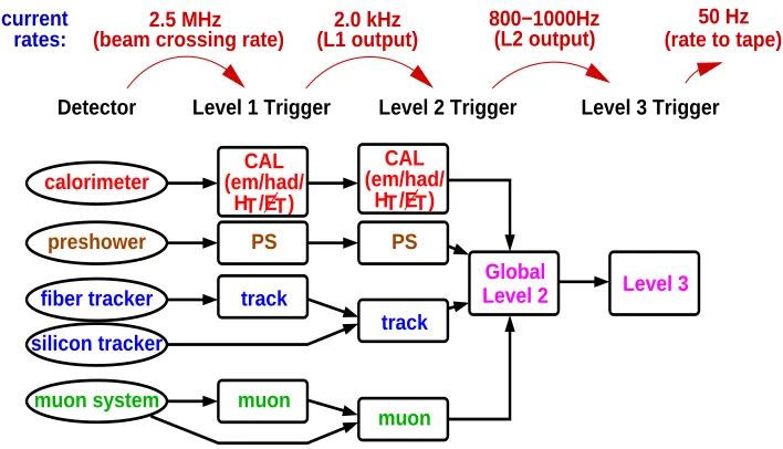
collisions are multijet events, while the production cross section of massive bosons, top quarks, or particles beyond the Standard Model is extremely small. To select these events, the trigger system is designed to select events with high transverse momentum jets or leptons. The DØ trigger system consists of three levels: Level 1 (L1), a pure hardware trigger using electronic signals from the detector, Level 2 (L2), using both electronic signals and reconstructed physics objects, and Level 3 (L3), a pure software trigger, using only reconstructed objects. A diagram of the trigger system is shown in Figure 2.9.

2.5 MHz

(beam crossing rate) (L2 output)

800−1000Hz 50 Hz

(rate to tape)

current rates:

CAL (em/had/

T H /E )_T

CAL (em/had/

T H /E )T

2.0 kHz (L1 output)

Detector Level 1 Trigger Level 2 Trigger Level 3 Trigger

calorimeter

preshower

muon system

fiber tracker

Global

muon

muon

PS PS

silicon tracker

track

track

Level 2 Level 3

Figure 2.9:Outline of the DØ trigger system.

Level 1 Trigger

The L1 trigger reduces the event rate from 2.5 MHz to about 2 kHz in about 4.2µs. It consists of

a luminosity trigger, a calorimeter trigger, a central-track trigger and a muon-system trigger. The luminosity system provides indication that a collision occurred, and the tracking system recon-structs tracks and stores seed track candidates to be used by other trigger units. The calorimeter performs a fast summation of electromagnetic and hadronic towers to look for towers that exceed a certain threshold. The muon triggers require coincidence between signals in layer A and either B or C.

Level 2 Trigger

The L2 trigger reduces the event rate to 1 kHz and takes about 100 µs to make a decision. The

2.2. The DØ Experiment 13

trigger, the L2 preshower trigger, the L2 muon-system trigger, the L2 SMT trigger, and the L2 central-track trigger.

Level 3 Trigger

The L3 trigger finally reduces the rate to about 50 Hz. This software trigger uses a simplified event reconstruction algorithm and is fully based on reconstructed physics objects.

The Data Acquisition System

3 Event Reconstruction and Simulation

Before triggered tt candidate events can be analyzed, physics objects, such as jets, leptons, muons¯

and missing transverse energy, need to be reconstructed from the raw data output of the detector. The measured energies and momenta of the decay products then allow an extraction of the top quark mass from the selected data sample. In order to study the properties of the data sample and to calibrate the method for the mass measurement, Monte Carlo simulated events are used. In the following sections, the reconstruction of the physics objects is described with a focus on objects used in this analysis: electrons (3.3), muons (3.4), jets (3.6), and missing transverse energy (3.8). The calibration of the charged leptons is discussed in Section 3.5, the calibration of the jets, in Section 3.7. At the beginning of this chapter, a brief description of the basic objects, such as tracks (3.1) and vertices (3.2), is given. After the reconstruction of the physics objects, the data quality criteria used at the DØ experiment are summarized in Section 3.9. The chapter ends with a discussion of the event simulation used to verify and calibrate the measurement technique.

3.1

Tracks

The reconstruction of tracks is one of the most important steps in the reconstruction of physical objects. Vertices are identified by clustering tracks, and the identification of electrons and muons requires a central track match, while photons are required to have no central track. In addition, the reconstruction of jets can be significantly improved by combining calorimeter and tracking information.

Charged particles passing the tracking detector leave hits in the detector that can be recon-structed as a track. The track finding is done in two steps. First of all, a set of track candidates is made using two different algorithms [27, 28]. Finally, the combined candidate list is passed to a track fitter based on a Kalman Filter algorithm [29]. Removing ambiguities and refitting all tracks with the Kalman Filter, the final track parameters are calculated with proper uncertainties.

3.2

Vertices

Particles traveling through the detector cause tracks that originate in one vertex. The so-called primary vertex (PV) represents the point of the hard interaction of the proton and antiproton, while the secondary vertices (SV) correspond to decaying heavy hadrons. The exact knowledge of vertices is important to determine precisely the direction of any calorimeter object.

3.3. Electrons 15

3.2.1 Primary Vertex

The primary vertex is defined as the interaction point of the proton and antiproton. A reliable reconstruction of the primary vertex is needed to distinguish objects from the hard interaction and the inelastic scattering. The primary vertex is reconstructed in three steps using the Adaptive Vertex Fitting [30]. First of all, tracks with a minimum transverse momentum of 0.5 GeV and at least two hits in the acceptance region of the SMT are selected. Then, all tracks of a cluster within 2 cm around the beam axis are constrained to a common vertex, and the vertex position, as well as all track parameters are recalculated. The fitting is repeated until theχ2_{distance of all tracks}

to the fitted vertex converges. Finally, the hard scattering vertex is selected as the vertex with the lowest probability to arise from a collision without hard interaction, i.e. with low transverse momentum [31].

3.2.2 Secondary Vertex

Heavy hadrons travel up to several millimeters in the detector before they decay. The decay results in a secondary vertex displaced from the primary vertex. Thus, secondary vertices can be used to detect heavy hadrons and to identify jets from the decay of a b hadron. The reconstruction of

secondary vertices is based on a Kalman Filter [32] and consists of four steps. First of all, jets are reconstructed based on tracker information only, then a list of tracks from these jets is selected, the vertex finding is performed, and the secondary vertices are finally selected.

3.3

Electrons

Electrons are identified as narrow clusters in the electromagnetic calorimeter, where all towers in a cone of radius∆R=0.2 around the most energetic seed are numbered among the cluster. The

cluster is required to have a minimum transverse energy of 1.5 GeV.

Since electrons lose most of their energyEtotin the electromagnetic calorimeter, the cluster is

required to deposit 90% of its energy in the electromagnetic layersEEM. In addition, the cluster

has to be isolated, i.e. no significant additional activity in a cone of radiusR=0.4 is allowed,

Etot(R<0.4)₋EEM(R<0.2)

EEM(R<0.2) < 0.15. (3.1)

To distinguish electrons from other particles, the shower of each electron candidate is compared to average distributions from simulated electron showers, and aχ2_{as a measure of compatibility}

is assigned. An electron candidate must fulfillχ2_{<50. As electrons are charged particles, at least}

one reconstructed track with a transverse momentum of at least 5 GeV is required to point to the cluster of the electron candidate with

|∆η| × |∆Φ| < 0.05_×0.05. (3.2)

The major remaining background arises from photons which happen to overlap with a track from a nearby charged particle. To discriminate against this background, an electron likeli-hood LEM,7 is calculated using seven different variables [33]. Electrons are required to have

16 3. Event Reconstruction and Simulation

Because of the poor energy resolution of electrons reconstructed in the inter-croystat region, electron candidates with a pseudorapidity between 1.1 and 1.5 are rejected. To suppress multiple scattering background, electrons are also not allowed to exceed a pseudorapidity of 2.5.

Comparing the reconstructed mass peak inZ_→ eedata and Monte Carlo simulated events,

a better resolution and a shifted peak has been observed in Monte Carlo. Hence the electron energies in Monte Carlo simulated events have to be smeared and scaled accordingly to reproduce the data [34].

3.4

Muons

The reconstruction of muons uses information from both the muon system and the tracking detec-tor. The former provides an unambiguous identification of the muon, the latter a precise measure-ment of its momeasure-mentum.

To discriminate muons against misidentified hadrons, the central track of the muon in the tracking chamber extrapolated to the muon system is required to match the reconstructed track in the muon detector. In addition, muon candidates are required to lie in the fiducial region of the muon system, i.e. the pseudorapidity must be less than 2. According to the number of wire and scintillator hits in the muon system and the quality of the matched track, muons are classified into different muon and track qualities, which are described by P. Calfayanet al. [26].

To reduce the number of non-isolated muons from semimuonic heavy-hadron decays in jets, a distance of at least 0.5 inRbetween the reconstructed muon and all jets in the event is required.

For tight isolated muons two additional isolation criteria are applied. One variable is computed by summing up the energies of the reconstructed tracks, the other variable is derived from energy deposited in the calorimeter. For background muons, the size of either of these sums is correlated with the muon energy, while for signal, it is not. Therefore, scaling the sums by the transverse muon momentum generates variables that tend to be higher for background than for signal. The track-based variable is computed as

εtrk

halo = _p1µ

T∆R

∑

ptrk_T , (3.3)

where the track matched to the muon is excluded from the sum. Similarly, the calorimeter-based isolation is defined as

εcal_halo = 1

pµ_T0.1<

∑

cell

T , (3.4)

where the sum is over individual calorimeter cells. Tight isolated muons are required to have values of bothεtrk

halo andεcalhalo that are less than 0.15.

Cosmic ray muons are rejected by requiring a timing window of 10 ns for all hits in the scintillator starting at the expected time of arrival from the hard interaction point. If any hit in the three layers lies outside this window, a muon is tagged as cosmic.

3.5. Calibration of Charged Leptons 17

3.5

Calibration of Charged Leptons

The calibration of electrons and muons is done usingZ_→ eeorZ_→µµevents, as well ascc¯and bb¯ resonance decays. These events have a clear back-to-back signature in the detector and can be

identified with low backgrounds. The energy of the electrons is measured in the electromagnetic calorimeter, the momentum of the muons, in the central tracking chamber, and thus both can be calibrated.

The total efficiency to reconstruct an electron or a muon is the product of several contribu-tions: the trigger efficiency, the efficiency of track identification, and the efficiency of applied quality cuts. All individual efficiencies are measured with the so-called tag-and-probe method using Z_→ eeor Z_→µµ events. Here, the criterion to be studied is only applied to one of the

leptons. The fraction of selected events where the second lepton also fulfills this requirement then yields a measurement of the efficiency. An illustration of this procedure is shown in Figure 3.1.

track ??

’’ µ ‘‘TAG −

µ

central track > 30 GeV

T

p isolated

µ > 15 GeV T p

’’ µ ‘‘PROBE −

’’ µ ‘‘TAG −

muon identified in the trigger and offline

muon identified − in the trigger? − offline? central track

> 30 GeV T p

isolated

isolated

> 20 GeV T p

’’ µ ‘‘PROBE −

central track

Figure 3.1: Illustration of the tag-and-probe method [35]; left: measurement of the tracking efficiency; right: identification of a muon in the trigger system and offline.

3.6

Jets

Quarks and gluons hadronize immediately and form showers of mesons and baryons in the hadronic calorimeter. The more energetic the parton is, the tighter the final hadrons are con-centrated around the direction of the parton. At the DØ experiment, a cone algorithm with a radius of∆R=0.5 is used to reconstruct jets [36]. The transverse energy of a jet relative to the beam line

is defined under the assumption that it originates at the primary vertex position.

The reconstruction of jets is done in three steps. First of all, preclusters are formed from calorimeter towers. Then, all preclusters are associated iteratively with a jet until the energy weighted center of the so-called proto jet is stable. Finally, the proto jets get either split or merged according to their energy overlap. All reconstructed jets with a transverse energy of less than 6 GeV are removed.

18 3. Event Reconstruction and Simulation

in the coarse hadronic calorimeter to be less than 40%. To suppress jets clustered around single cells that fired erroneously, two additional cuts are applied. First, the hot fraction, i.e. the energy ratio of the highest to the next-to-highest calorimeter cell assigned to a jet, must be less than 10%. Secondly, it is not allowed that a single cell contains 90% of the total jet energy. Far forward jets with a pseudorapidity of more than 2.5 are eliminated to reduce background from beam remnants. The cut values quoted above refer to jets measured in the central region of the detector. A detailed list of the cut values for the different detector regions is given by A. Harel [37].

Jets with a distance of less than 0.5 inRto a high energetic electromagnetic object are rejected.

3.7

Jet Energy Scale

For any measurement at app¯collider, it is mandatory to have a good knowledge of the jet energy

scale (JES) and the jet resolution. Their determination is more difficult than that for a charged lepton and the uncertainties on the jet energy scale and resolution are the dominant source of systematic uncertainty in the measurement of the top quark mass.

Figure 3.2:Evolution from a parton to a calorimeter jet[38].

3.7.1 Overall Jet Energy Scale

The goal of the jet energy scale is to correct the energy of the calorimeter jet back to the one of the stable-particle jet before any interaction with the detector took place, see Figure 3.2. After this is done for both light andbjets, an additional correction is applied to jets from bottom quarks. The

3.7. Jet Energy Scale 19

Energy Offset EO

EOrepresents an offset to the jet energy that includes contributions from noise coming from

elec-tronics and radioactive decays of the uranium absorber, additional pp¯interactions, and previous

crossings. The energy contributed by the spectator quarks to the hard-scattering process, the so-called underlying event, is not included in the offset as it already affects jets at the particle level. The offset energy depends on the cone size of the jet, its pseudorapidity with respect to the primary vertex, the number of reconstructed vertices and the instantaneous luminosity.

The offset is estimated from the energy density in minimum-bias and zero-bias events. Minimum-bias events are triggered by the luminosity monitors signaling the presence of a po-tential inelastic proton-antiproton collision. Their energy density is a measure for the effect from multiple proton-antiproton collisions. To eliminate contributions from the spectator quarks, the difference of the energy density in events with more than one primary vertex and exactly one primary vertex is used. Zero-bias events are triggered at every bunch crossing with the explicit requirement of no vertex in the event. Their energy density is a measure of contributions from pile-up, electronics, and uranium noise.

The energy offset of a jet with cone radius 0.5 is shown for different primary vertices as a functions of its pseudorapidity in Figure 3.3.

jet

η

-3 -2 -1 0 1 2 3

Offset Energy [GeV]

0 5 10 15 20 25 30

NP NP+1MI NP+2MI NP+3MI NP+4MI

DØ Run II RCONE=0.5

Figure 3.3:Offset energy for a cone radius of 0.5 as a function of the jet pseudorapidity [38]. The different lines show the prediction for the offset energy from noise and pile up (NP) and multiple interaction (MI).

Absolute Calorimeter Response R

The largest correction is the one that accounts for the calorimeter response of the jet. It is measured inγ+jet events where the detector response of the photon is known with little uncertainty from Z_→ eeevents.

The so-called MissingET Projection Fraction method (MPF) allows a measurement of the

calori-meter response from the pT imbalance in the event. In the calorimeter, the response of the photon

20 3. Event Reconstruction and Simulation

calorimeter

R_γ~pγ_T+Rhad~phad_T = ₋~p/T, (3.5)

whereRγ~pγ_Tcorresponds to the measured photon momentum, andRhad~phad_T , to the jet momentum.

Taking into account that the true hadronic recoil and the photon momentum balance each other, Equation (3.5) can be written as

R_had

Rγ = 1+

~p/T·~pγT

~pγ_T2 . (3.6)

Thus, the response of the hadronic recoil relative to the response of the photon can be estimated from the photon momentum and the projection of the imbalance of the transverse momentum~p/T

onto the direction of the photon in the transverse plane.

The absolute response measurement is performed using events with one single photon candi-date in the central region of the detector, and exactly one jet with an absolute pseudorapidity of less than 0.4. The photon and the jet are required to be back-to-back, so∆φ(γ,jet)>3.0.

Since the energy resolution of jets is broader than the one of photons, the dependency on the true jet energy is estimated from the transverse energy of the photon by

E0 = pγ_T cosh(η_jet), (3.7)

where ηjet is measured with respect to the reconstructed primary vertex. The estimator E0 is

strongly correlated with the particle-level-jet energy since it is calculated using the transverse momentum of the photon and the direction of the jet which are measured with good precision. The energy dependence of the jet response is described by a quadratic logarithm function.

R(E0) = p0+p1log(E0/100(GeV)) +p2log(E0/100(GeV)). (3.8)

Due to uncertainties in the detector simulation, the calorimeter response is measured separately in data and Monte Carlo simulated events. The response for jets with a cone radius of 0.5 inγ+jet

data events is shown in Figure 3.4. Extrapolating the fit to very high jet energies, the response uncertainty is about 2%.

Relative Calorimeter Response Fη

While the central part and the end caps of the calorimeter are almost uniform, the region in between is not as well instrumented which causes a non-uniformity in the response as a function of the pseudorapidity. The relative response correction aims to calibrate forward jets with respect to the central ones, and gives the final response correction in combination with the absolute scale.

The relative response is measured as the absolute response in γ+jet data and Monte Carlo

events using the Missing ET Projection Fraction method. The tag object, i.e. the photon, is

required to have a pseudorapidity of less than 0.4, and the response of the probe jet is determined using a fine binning of the pseudorapidity (mostly about 0.1). The relative response as a function of the pseudorapidity for different values of the energy estimatorE0 defined in Equation (3.7) are

depicted in Figure 3.5. As expected, the correction is largest in the region of 1.0<_|η_|<1.5. Due

3.7. Jet Energy Scale 21 jet R 0.60 0.65 0.70 0.75 0.80 0.85 = 0.5 cone R

| < 0.4 jet det η | +jet ptcl γ

/ndf = 1.65 2

χ

E’ (GeV)

30 40 100 200 300

rel. difference (%) _-4-3 -2 -1 0 1 2 3 4 stat.

DØ Run II

Figure 3.4:Measured response inγ+jet data events for a jet cone size of 0.5 [38].

The estimated uncertainties on the relative response are shown on the right side of Figure 3.5. The dominant uncertainty arises from imperfections on the energy-dependent parameterization and η interpolation (average residuals). In the very forward region, there is also a significant contamination from background.

jet det η

-3 -2 -1 0 1 2 3

η +jet γ F 0.60 0.65 0.70 0.75 0.80 0.85 0.90 0.95 1.00 1.05 1.10

E’ = 25 GeV E’ = 50 GeV E’ = 100 GeV E’ = 200 GeV E’ = 400 GeV E’ = 700 GeV

= 0.5 cone R

DØ Run II

|

jet det η

|

0.0 0.5 1.0 1.5 2.0 2.5 3.0 3.5

[%]_η /F η F ∆ -3 -2 -1 0 1 2 3 +jet γ = 0.5 cone R total

stat. at pT’ = 50 GeV/c average residual

background corr. at pT’ = 50 GeV/c

Figure 3.5: Left: measured calorimeter response as a function of the pseudorapidity for different values of

the jet energy estimatorE0inγ+jet data events; right: corresponding uncertainties [38].

Showering S

22 3. Event Reconstruction and Simulation

showers in the calorimeter and the finite size of calorimeter cells. Typically, the net correction is smaller than unity. It strongly depends on the cone size of the jet and its pseudorapidity with respect to the primary vertex. The showering correction is measured separately in data and Monte Carlo simulatedγ+jet events. To reduce the impact of multiple interactions, exactly one primary

vertex is required.

First, the jet energy density profile from calorimeter towers is measured as a function of the radial distance to the jet axis. Then, templates of various contributions to the jet profile from Monte Carlo simulated events are fitted to the measured jet profile adjusting the relative size of the specific pro-file source. Finally, the showering correction is determined as the ratio of the visible energy in the jet cone to the visible energy of all particles from the particle jet. In Monte Carlo simulated events, the showering correction also can be determined using information about the energy de-posit of each particle in the different calorimeter cells. The results are in good agreement with the template-based method.

The size of the showering correction is shown in Figure 3.6. It is much bigger for forward than for central jets, as the solid angle of a jet decreases with increasing jet rapidity making the detector showering effects more important.

E’ (GeV)

810 20 30 100 200 1000

shower

F

0.80 0.85 0.90 0.95 1.00 1.05 1.10

DØ Run II

= 0.5 cone R

0.0 < | | < 0.4η 0.4 < | | < 0.8η 0.8 < | | < 1.2η 1.6 < | | < 2.0η 1.2 < | | < 1.6η

2.0 < | | < 2.4η

3.2 < | | < 3.6η 2.8 < | | < 3.2η 2.4 < | | < 2.8η

Figure 3.6: Showering correction for jets with a cone size of 0.5 in data as a function of the jet energy

estimatorE0[38].

Remaining Bias kbias

To achieve an accuracy on the order of 2%, an additional factor is applied to correct for the major remaining biases.

3.7. Jet Energy Scale 23

Moreover, additional activity in the event or the splitting and merging of jets can bias the measurement of the jet response. These effects have been studied using Monte Carlo simulated events where individual particle energy depositions in different calorimeter cells can be used to compute the true jet response to which the response from the Missing ET Projection Fraction

method can be compared.

Taking all corrections into account, the true energy of the particle jet,Ecorr, can be calculated

from the measured jet energy,Emeas, as

Ecorr = Emeas−E0

R_·F_η·S ·kbias , (3.9)

whereE₀,R,F_η,Sandk_biasare the corrections described above.

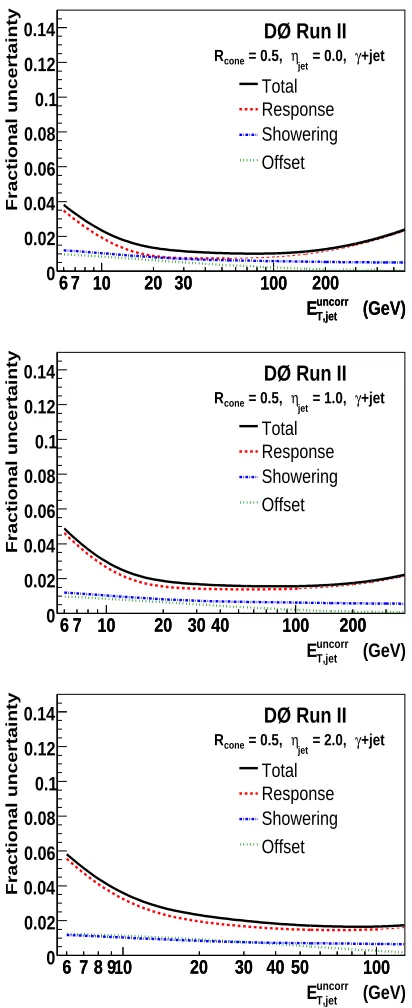
The relative uncertainty on the jet energy scale in data as a function of the energy estimator

E0 is shown in Figure 3.7 for jets with a cone size of 0.5 and three different pseudorapidity bins

of 0.0-0.5, 1.0-1.5, and 2.0-2.5. Besides the total relative uncertainty, the contributions from the different subcorrections are displayed, where the relative and the absolute response corrections have been lumped together. The relative uncertainty is mainly caused by the uncertainty on the response, especially at low and high transverse energies. The dominant source here is the uncer-tainty on the photon energy scale coming from the absolute scale unceruncer-tainty from theZ_→ ee

mass peak and the relative electron-to-photon scale uncertainty. At low transverse energies and in the very forward region, the background contamination inγ+jet events plays an important role,

at high transverse energies the main problem is the limited statistics to constrain the high energy extrapolation. All technical details and studies regarding the Run II JES are given by A. Juste

24 3. Event Reconstruction and Simulation

(GeV) uncorr T,jet E

6 7 10 20 30 100 200

(GeV) uncorr T,jet E

6 7 10 20 30 100 200

Fractional uncertainty 0 0.02 0.04 0.06 0.08 0.1 0.12 0.14 Total Response Showering Offset DØ Run II

+jet γ = 0.0, jet η = 0.5, cone R (GeV) uncorr T,jet E

6 7 10 20 30 40 100 200

(GeV)

uncorr T,jet

E

6 7 10 20 30 40 100 200

Fractional uncertainty 0 0.02 0.04 0.06 0.08 0.1 0.12 0.14 Total Response Showering Offset DØ Run II

+jet γ = 1.0, jet η = 0.5, cone R (GeV) uncorr T,jet E (GeV) uncorr T,jet E

6 7 8 910 20 30 40 50 100

(GeV)

uncorr T,jet

E

6 7 8 910 20 30 40 50 100

Fractional uncertainty 0 0.02 0.04 0.06 0.08 0.1 0.12 0.14 Total Response Showering Offset DØ Run II

+jet γ = 2.0, jet η = 0.5, cone R (GeV) uncorr T,jet E

Figure 3.7:Relative uncertainty on the jet energy scale for jets with a cone radius of 0.5 in data as a function

of the uncorrected transverse energy and three different pseudorapidity bins; top: 0.0<|ηjet|<0.5; middle:

1.0<|ηjet|<1.5; bottom: 2.0<|ηjet|<2.5. Besides the total fractional uncertainty, the one from the

3.8. Missing Transverse EnergyE/T 25

3.7.2 Bottom Quark Jet Energy Scale

Jets from bottom quarks and light-flavor jets, i.e. all jets not initiated by a bottom quark, show different frequencies in the production of hadrons and their momentum spectra. Thus, the ratio of electromagnetic and hadronic energy is different for both kinds of jets leading to a different response. In addition, bjets may contain a semileptonic heavy-hadron decay causing a different

response in case this decay is not detected. An explicit correction of the jet energy is applied when the charged lepton is identified inside the jet. Due to the large mass of a bottom quark, the showering for light-flavor andb jets is also different. So far, there is no certified jet energy

scale for jets initiated frombquarks at the DØ experiment. Thus, the overall jet energy scale is

used for both light-flavor andb jets and the additional systematic uncertainty is assigned to the

reconstructed energy ofbjets.

3.7.3 Jet Energy Resolution

The jet energy resolution is measured usingγ+jet andZ+ jet events [40]. Its parameterization is

given in Equation (2.3). Comparing the energy resolution in measured and simulated events, the resolution of the simulated jets needs to be smeared and shifted to reproduce the data. In addition the reconstruction and identification efficiencies are different for data and Monte Carlo simulated events, such that some of the simulated jets need to be discarded. All this is done in the so-called Jet Shifting, Smearing and Removal (JSSR) [41].

3.8

Missing Transverse Energy E

/

Since neutrinos escape the detector without any interaction, they can only be identified indirectly by the imbalance of the transverse momentum of the event. The missing transverse momentum is calculated from the vector sum of all calorimeter cells1 _{which pass the T42 algorithm [42].}

The missing momentum vector is corrected for the jet energy scale and the scale of any charged lepton in the event. In addition, it is corrected for the energy loss of muons in the calorimeter through ionization that is substantially smaller than the muon momentum measured in the tracking chamber.

The unclustered transverse energy is defined as the magnitude of the vector sum of the trans-verse momenta of all calorimeter objects that are not assigned to a jet or a charged lepton.

3.9

Data Quality

In order to ensure a good data quality, the following selection criteria are applied. A whole run or luminosity block, see Section 2.2.5, is excluded if one of the subdetector systems is declared as bad during data taking. In addition, a list of bad luminosity blocks is created based on certain calorimeter information that is checked per luminosity block. Events belonging to a bad luminosity block are discarded.

In addition, there are calorimeter noise patterns, for which single events are discarded. The noise patterns include the so-called noon noise, which is caused by external noise, coherent noise,

1_{Due to the large noise in the coarse hadronic layers, cells here are only considered if clustered into a reconstructed}

26 3. Event Reconstruction and Simulation

where for all crates a synchronous shift in the pedestals occur, and ring of fire, where a ring of energy in the transverse plane occurs based on grounding problems. Events are tagged with empty crates in case one of the crates could not be read out.

3.10

Monte Carlo Simulation

Monte Carlo (MC) simulation is one of the key tools in experimental high energy physics. It is used for several purposes in the present analysis. First of all, Monte Carlo events are used to optimize the selection of tt¯events, and to check the sample composition of the selected data

sample. Secondly, simulated events are used to calibrate the method for measuring the top quark mass, and to compare the expected uncertainties to the measured ones.

The simulation of Monte Carlo events is based on the leading-order matrix element of the con-sidered process. The MC generator ALPGEN [43] is used to generate the hard parton-scattering

process for the signal processtt¯and the main background process(Z_→ττ) +jets. PYTHIA[44]

is used to simulate the background processes involving two weak vector bosons (WW+jets, W Z+jets). The simulation of the hard-scattering process is interfaced with PYTHIA to model

initial- and final-state gluon radiation. To avoid an overlap of the phase-space regions covered by the hard-gluon radiation and the gluon emission from the matrix-element calculation, a matching procedure [45] has been used. PYTHIAis also used to model the fragmentation and

hadroniza-tion. They are interfaced with EVTGEN[46] and TAUOLA [47] to describe the heavy hadron and

τlepton decays.

Afterwards, the MC simulated events are processed with a detailed simulation of the DØ detector based on GEANT[48], and the same reconstruction and selection criteria as for the data

are applied.

Depending on the instantaneous luminosity, more than one pp¯collision may take place in the

same bunch crossing. To simulate this effect, minimum-bias events are measured, and added to the simulated events. In a similar way, pile-up of signals from previous collisions is recorded with a random trigger and added.

4 The Top Quark and the Concept of Mass

The present chapter describes the fundamental elements of this thesis: the top quark and the concept of mass. After a short review of top quark properties in Section 4.1, its production (4.2) and decay (4.3) are described. Afterwards, different concepts of mass and the relevance of the top quark mass are discussed in Sections 4.4 and 4.5. The chapter ends with a short overview of different mass measurement concepts.

4.1

The Top Quark within the Standard Model

When the bottom quark was discovered in 1977, the Standard Model of particle physics [49, 50] predicted the top quark as the weak-isospin partner of the bottom quark. Indirect evidence for the top quark became compelling over the years, and constraints from electroweak data [3] pointed exactly to the range where the top quark was finally discovered 18 years later. The discovery of the top quark in 1995 by the CDF [1] and DØ experiments [2] was a great success for the Standard Model, but compared to the other quarks and leptons far less is known about the top. The strong interaction is mostly studied in the pair production of top quarks, the weak interaction, in its decay and in the production of single top quarks. An overview of the particles in the Standard Model as well as their masses is given in Figure 4.1.

Four fundamental parameters of the Standard Model are directly associated with the top quark: its mass and the three CKM matrix elements involving top. With the current world average of 172.4_±0.7(stat.)_±1.0(syst.)GeV [8], the top quark is the heaviest of the observed fundamental

particles and it is often discussed to play a special role in the electroweak symmetry breaking. Besides the large mass of the top, the top quark is also unique due to the theoretical expected lifetime of 5·10−25s [6], where the experimental bound is_cτtop<52_µm at 95% C.L. [52]. The

top quark is predicted to decay so quickly that it cannot hadronize and the spin of the top is not depolarized by chromomagnetic interactions within bound states. Thus, it is possible to measure observables which depend directly on the spin of the top quark giving an excellent test of the Standard Model.

The electric charge of the top quark is predicted by the Standard Model to beQ= +2/3, but

is not yet measured. Thus, the fact that the discovered particle at the Tevatron could be an exotic quark with charge Q=₋4/3 decaying into a negatively chargedW boson and bottom quark is

only excluded at the 92% C.L. [53].

In the Standard Model, the top quark is predicted to have the same V-A charged current weak interaction as the other fermions. In the limit of a massless bottom quark, thebquark has to be

left-handed, so that theW boson cannot be right-handed assuming angular momentum conservation

and the top quark to be a spin-1/2 particle. Since the coupling of the top quark to a longitudinal (zero helicity)W boson is similar to its Yukawa coupling, the branching ratio is predicted to be

28 4. The Top Quark and the Concept of Mass

Figure 4.1:Overview of the leptons and quarks within the Standard Model as well as the gauge-mediating bosons and the yet-unobserved Higgs boson [51]. The particles are ordered according to their mass. Two particles in the Standard Model are massless: the photon and the gluon.

about 70%. The by-now most precise measurement yields a branching ratio of−0.03_±0.07 for

the coupling of the top quark to a right-handedW boson, and 0.66_±0.16 for the longitudinal. So

both measurements are in perfect agreement with the Standard Model.

4.2

Top Quark Production

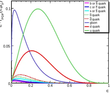
Until the start of the LHC in 2009, the Tevatron collider is the only place on Earth where top quarks can be produced directly. Due to the high energies, the production can be described by quantum chromodynamics and factorized in three different parts: the modeling of the partons of the incoming hadrons, the hard-scattering process of two partons, and the hadronization of the final-state particles. A schematic illustration of these parts is given in Figure 4.2. The constituents of the colliding hadrons are modeled using the so-called parton distribution functions (PDFs). The PDF fPDF(ε,µ2_F)describes the probability to find a gluon or quark of given flavor with longitudinal

momentum fraction εwithin the colliding parton. The factorization scaleµ2_F denotes the energy

region where the PDFs are probed and finally allows the separation of the parton modeling and the hard-scattering process. Since the PDFs cannot be calculated directly, they have to be measured in fits to experimental data [54]. As an example, the CTEQ6L1 parameterization at a scale of

µF=170 GeV used in the present analysis is shown in Figure 4.3.

4.2. Top Quark Production 29

P

ε_{1 1}

P

ε_{2 2}

PDF µF2 f ( , )ε₁

PDF µF2 f ( , )ε2 P 1

P₂

(Q )

σ^ 2

2 1

hadronization

Figure 4.2: Schematic illustration of a hard-scattering process between two hadrons. Due to the high en-ergies the internal structure of the colliding hadrons can be resolved, and the hard interaction takes place

between the two partons with momentum fractionsε1P1andε2P2from the incoming hadrons with

momen-tumP1andP2. The partonic cross section ˆσcan be calculated perturbatively using the factorizationµFand

the renormalization scaleµR. The formation of the final-state particles cannot be calculated in perturbation

theory, but again is independent of the hard interaction.

∈ 0 0.2 0.4 0.6 0.8 1

)

2 F

µ

,

∈

(

PDF

f

⋅

∈

0 0.05 0.1

quark b b or

quark c c or

quark s s or

quark u

quark d gluon d quark u quark

Figure 4.3: CTEQ6L1 parametrization of the parton distribution functions depending on the momentum

fractionεof the parton. The factorization scaleµFis chosen to be 170 GeV.

top quarks are produced via the electroweak one. The leading-order Feynman diagrams for both production processes are shown in Figures 4.4 and 4.5.

Thett¯production cross section is given by

σ=

∑

p1,p2 Z

dε1dε2fPDF(ε1,µ_F2)fPDF(ε2,µ2_F)σˆ

ε1,ε2,αS µ2F

,Q

2

µ2_R

, (4.1)