The influence of numerical models on determining the drag coefficient

The influence of numerical models on determining the drag coefficient

Josef Dobeš1,a, Milada Kozubková1,b

1

Department of Hydromechanics and hydraulics equipment, Technical University of Ostrava, Ostrava, Czech republic

Abstract. The paper deals with numerical modelling of body aerodynamic drag coefficient in the transition from laminar to turbulent flow regimes, where the selection of a suitable numerical model is problematic. On the basic problem of flow around a simple body – sphere selected computational models are tested. The values obtained by numerical simulations of drag coefficients of each model are compared with the graph of dependency of the drag coefficient vs. Reynolds number for a sphere.Next the dependency of Strouhal number vs. Reynolds number is evaluated, where the vortex shedding frequency values for given speed are obtained numerically and experimentally and then the values are compared for each numerical model and experiment. The aim is to specify trends for the selection of appropriate numerical model for flow around bodies problem in which the precise description of the flow field around the obstacle is used to define the acoustic noise source. Numerical modelling is performed by finite volume method using CFD code.

1 The basic problem definition

For the drag coefficient numerical modelling is selected the basic problem of flow around sphere by given diameter. The diameter of the sphere is 36 mm, relative roughness of the sphere surface is 0 (smooth body). The aim of modelling is to compare the drag coefficient values Cd computed numerically with the values reported

in the literature [1, 2] for the range of Reynolds number Re = 23000 to 230000, where the experimentally obtained data is consistent from multiple authors. The drag coefficient Cd is given by equation [1]:

S u

F C

⋅ ⋅

⋅

= ₂D

d

2

ρ (1)

where FD represents the drag force component parallel

with velocity u in the flow direction, ȡ is density of fluid flowing around the object and S is the largest surface perpendicular to the main flow direction of velocity u. Also Strouhal number is compared in relation on Reynold number, St = f (Re), by vortex shedding frequency obtained by finite volume method and experimental measurement in wind tunnel. Strouhal number calculation can be [2]:

u l f

St= ⋅ (2)

where f presents vortex shedding frequency, l characteristic dimension (diameter sphere) and u velocity.

2 Turbulence mathematical models

Modelling of turbulence is still in the research stage,

which is constantly changing with the progress in the mathematical, physical and technical sectors. In numerical simulation of turbulent flow theory, there are three different approaches that result from simplifying modifications of the starting equations describing the flow, and a method of direct simulation (DNS), which is almost unusable for technical reasons, the method of time-averaging (RANS), which is highly used in engineering applications, but least accurate method and a large vortex method (LES), which is some compromise between the DNS and RANS. We have made a complex comparison of RANS and LES models that are available in the ANSYS FLUENT [3], while the best results of the RANS group drawn Transition k-kl-omega model and from the LES group we should be able to choose more results, but to illustrate LES Lilly Smagorinski model and LES WALE model were selected.

2.1 Transition k-kl-omega model

This model [6] can be used for exact numerical solution of boundary layer transition from laminar flow regime to turbulent flow regime. It is considered a three linear equation model of vortex viscosity, where transport equations are defined for time-averaging quantities, while the minutes are used Einstein's summation rule. Continuity equation for incompressible fluid has the form [5]:

0

j j ₌

∂ ∂ x u

where member uj represents j-th velocity component,

index j expresses the summation index.

Navier - Stokes equations for incompressible fluid:

i 2 j i 2 i i 1 D D f x u x p t u + ∂ ∂ ⋅ + ∂ ∂ ⋅ − = ν

ρ (4)

where member t D

D

indicates substantial derivative,

which is a kind of total derivatives, tracking movement. In addition, a member Ȟ represents the kinematic viscosity, ui is i-th velocity vector component, p denotes

pressure, ȡ the density of fluid and member fi represents

i-th component of the general external body force (gravity, centrifugal force) [5].

Transition stress model further defines turbulent kinetic energy kT:

¸ ¸ ¹ · ¨ ¨ © § ∂ ∂ ¸¸¹ · ¨¨© § ₊ ∂ ∂ + − ⋅ − + + = j T K T j T T NAT K T T D D x k a a x D k R R P t k ν ω (5)

Laminar kinetic energy kL is defined:

¸ ¸ ¹ · ¨ ¨ © § ∂ ∂ ⋅ ∂ ∂ + − − − = j T j L NAT K L L D D x k x D R R P t k

ν (6)

and inverse turbulent timescale Ȧ:

(

)

Ȧ1 1

D D T x a a x d k f a f C C R R k f C P k C t ω ν ω ω ω ω (7)

More details about this model are discussed in literature [6]. Using Ȧ as time scale defining the variable can reduce the effect of discontinuities in the outer region of the turbulent boundary layer and thus eliminate the transition region in the velocity profile.

2.2 LES Lilly Smagorinski model

The LES method solves directly large eddies, while small eddies are modelled. LES thus falls between DNS and RANS methods at a fraction of the time solved. Justification of LES method can be summarized as follows:

• momentum, mass, energy, and other scalars are moved mainly to large vortices,

• larger vortices are more dependent on the problem. They are determined by the geometry and boundary conditions of flow,

• small vortices are less dependent on the geometry, tend more towards isotropy, therefore they are more general or universal (they are present in every turbulent flow) [5].

The basic principle of LES is the decomposition of the large and small scales and filtration. The result is the Schumann method leading to the following form of the equation for the distribution of flow and temperature fields. 0 j j = ∂ ∂ x u (8)

(

)

j i j j i j i i 1 D D u u x x u x u x x p t u − ∂ ∂ + °¿ ° ¾ ½ °¯ ° ® ­ » » ¼ º « « ¬ ª ∂ ∂ + ∂ ∂ ⋅ ∂ ∂ + ∂ ∂ ⋅ − = ν

ρ (9)

From the filtering operations subgrid turbulent stress scale IJij issued as unknown which must be modelled.

Subgrid scale using Boussinesq hypothesis as in the RANS models, subsequently subgrid turbulent stress scale is modelled by equation:

ij t ij kk ij 2 3 1 S ⋅ ⋅ − = ⋅ ⋅ − τ δ μ

τ (10)

where the isotropic part of subgrid scale stress IJkk is not

modelled, but it adds to the filtering expression for the static pressure. Sij is the strain rate tensor for the resolved

scale [6]. μt is subgrid scale of the turbulent viscosity, where the first simple model was designed by Smagorinski. It defines the scale turbulent viscosity:

S L ⋅ ⋅ = 2 s t ρ

μ (11)

where Ls is the mixing length for subgrid scale and S

the size of the strain rate tensor for resolved scale [6].

2.3 Wall-Adapting Local Eddy model (WALE LES)

This model was desingned in 1999 by Nicoud and Ducros. It governs the relationship of scale modelling of turbulent viscosity μt [6]. Furthermore, it provides even more accurate expression for the stress tensor speed SijD.

This model is suitable for a wide range of applications.

3

Computing mesh, Calculation

structure, boundary conditions

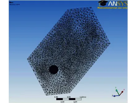
3.1 Computing mesh

Computing mesh is created in the program Ansys Workbench – Ansys Meshing by method Patch Conforming Method – Tetrahedrons. There is also made cylindrical mesh compression for the better rendering of vortex structures, and also because of the saving of the total cells number, the other area is meshing by coarser mesh.

On the surface flow past sphere boundary layer by First Layer Thickness is created of these defined parameters:

• height/thickness of the first boundary layer – 0.0005 m,

• number of layers – 10,

• growth scale of different layers from the first – 1.2. The number of grid cells is 484 279. They are the tetrahedral elements.

3.2 Calculation structure

Calculations for the three turbulent models will be selected for a velocity of 10 m s-1, 20 m s-1, 40 m s-1, 60 m s-1, 80 m s-1 a 100 m s-1, which covers the range investigated Reynolds number from 23000 to 230000. The calculation is performed as a time-dependent with time step ¨t = 0.0001 s, as an initial step the calculation with 2048 time steps is done, followed by the calculation itself containing 4096 time steps at the same time step ¨t. When calculating the 4096 steps the option to save data to evaluate the time-averaging variable is checked.

3.3. The boundary conditions

For all calculations basic conditions are given – gravitational acceleration g = 9.81 m s-2 in the direction – Y, when in the direction + X is given velocity u around the object, the atmospheric pressure, pATM = 98 kPa. At

the input the velocity condition velocity inlet is given and at the output the pressure condition - pressure outlet - is given. For turbulent model Transition k-kl-omega it is also necessary to define the input and output parameters of the hydraulic diameter dH:

O S

d_H =4⋅ (13)

and turbulence intensity IT[8]: 8 / 1 T 0,16

− ⋅

= Re

I (14)

and for this model it is necessary to define the value of laminar kinetic energy kL = 0.001 m

2

s-2, this value is the default and is the same for all the simulations using that model. Boundary conditions for LES models are set as follows: the input – velocity u, the output – gauge pressure p = 0 Pa.

4 Evaluation of the drag coefficient

C

and dimensionless criteria

y+

This section is an evaluation of the drag coefficient Cd for

the turbulence models and a comparison with values reported in the literature for a given range of Reynolds number, according to various authors numerically and graphically.

For the range of Reynolds number < 3Â105 Brauer defined drag coefficient Cd subsequently [4]:

4 , 0 4 24

d = + +

Re Re

C (15)

Newton defined the value of the drag coefficient for

The actual evaluation of the drag coefficient is performed for the directional vector of drag coefficient: Direction Vector – X = 1, Y = 0, Z = 0.

Prior to the evaluation it is needed, however, to set the correct reference values for calculating the drag coefficient. Their numeric values are given in Table 1, where all values outside the velocity will always be constant.

Table 1. Reference Values.

Quantity Value

Area 0.001017876 m2

Density 1.20391 kg m-3

Enthalpy 0 J kg-1

Length 0.036 m

Pressure 0 Pa

Temperature 293.15 K

Velocity 10, 20, 40, 60, 80, 100 m s-1

Viscosity 1.849Â10-5 Pa s

Ratio of Specific

Heats 1.4

In Table 2 drag coefficients Cd for various turbulence

models and the Reynolds number Re are evaluated together with the values reported in the literature [4].

Table 2. Drag coefficient.

Cd

Velocityu / Reynolds NumberRe

10 m s-1

23440 20 m s-1

46880 40 m s-1

93760 60 m s-1

140641 80 m s-1

187521

100 m s-1

234401 Transition

k-kl-omega 0.51 0.40 0.32 0.29 0.25 0.25 LES Lilly

Smagorinski 0.4 0.35 0.35 0.48 0.45 0.30 LES WALE 0.51 0.44 0.42 0.42 0.35 0.32 Newton 0.44 0.44 0.44 0.44 0.44 0

Brauer 0.43 0.42 0.41 0.41 0.41 0.41

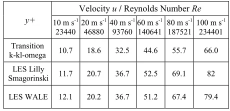
The values for the dimensionless criterion y+ at the wall of the object which is flown around object for each turbulence models are listed in Table 3.

Table 3. Non-dimensional criteria y+ for mesh.

y+

Velocityu / Reynolds NumberRe 10 m s-1

23440 20 m s-1

46880 40 m s-1

93760 60 m s-1

140641 80 m s-1

187521

100 m s-1

234401 Transition

k-kl-omega 10.7 18.6 32.5 44.6 55.7 66.0 LES Lilly

EPJ Web of Conferences

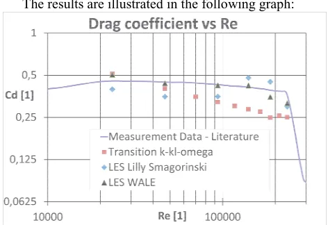
The results are illustrated in the following graph:

Figure 2. Drag coefficient for sphere.

5 Evaluation of the Strouhal number,

compared with the experiment

Strouhal number (Equation 2) can be evaluated using the frequency of vortex shedding behind flown-around body. The measurement and simulation involves scanning the instantaneous velocity at a precisely defined point in both numerical simulation and the experimental device. This comparison is done for speed u = 10 m s-1. Point X2 has the defined coordinates relative to the zero point, which is located in the center of flow-past sphere:

Table 4. Coordinates of measurement point X2.

Coordinates [m]

X Y Z

X2 0.09 0 0

In the program Ansys Fluent a measuring point with given coordinates will be specified, see Table 4, and the average speed will be recorded at a given point for each time step of the calculation (4096 time steps). Total time record in point is therefore 0.4096 s

The experiment was conducted on wind tunnel at the Department of Hydrodynamics and Hydraulics equipment Technical university of Ostrava. To measure the hot-wire anemometer was used, which works on the principle of convection heat transfer from the heated sensor (wire with a diameter of 5 mm) into the environment. The heat transfer is primarily dependent on the fluid velocity. Using sensors placed in the flow field of electronics and the feedback loop fluctuations rate of small scale and high frequencies can be measured. CTA probes usually have a tungsten wire, 1 mm long and 5 mm in diameter, mounted on two needle-shaped spikes. They can have 1, 2 or 3 wires. For liquids it is needed to cover the wires with a thin protective film. The measurement is performed using one-wire probe bent by 90 °, marked 55P14. The parameters for measuring by the hot-wire anemometer for subsequently performed spectral analysis are:

• sampling frequency - set to 120 Hz, where we assume the value of Strouhal number 0.2;

• the value of antialiasing filter set to 140 Hz frequency; here is the need to comply with Nyquist criterion;

• number of samples - 4096.

Figure 3. Probes type 55P14 for measurement one component of velocity perpendicular to probe axis [7]

The measured data was converted to a text file with the OUT extension due to the evaluation of FFT analysis in the Ansys Fluent. Data obtained by numerical simulation was also evaluated by the software; thereby avoiding error occurring while processing FFT by different software. After the FFT of the experimental data the vortex shedding frequency value was subtracted:

211752 . 0 10

036 . 0 82 . 58

82 .

58 MEAS

MAES MEAS

= ⋅ =

= ⋅ = →

=

u d f St

Hz f

(17)

The table 5 summarizes the values of frequencies obtained from the FFT and their corresponding Strouhal numbers calculated for different numerical models:

Table 5. Frequencies and Strouhal Number; u = 10 m s-1.

Quantity Unit

Numerical Model

Transition k-kl-omega

LES Lilly

Smagorinski LES WALE f Hz 20 65 40

St 1 0.072 0.234 0.144

From the comparison of the drag coefficient Cd

numerically, Table 2, or graphically, Graph 1, and comparison Strouhal number St, Table 5, it can be concluded that a for a comprehensive aerodynamic modelling task, according to the results the model LES Lilly Smagorinski appears to be the best. For modelling the drag coefficient Cd the LES WALE model gets the

results closest to the literature, but the value of vortex shedding frequency and the value of the Strouhal number is strongly underestimated in comparison with the value StMEAS (17). However, for the comprehensive comparison

6 Graphical results of the flow around

the sphere, comparison of turbulent

models

Graphically, it is possible to compare the distribution of the instantaneous velocity field and time-averaging velocity field for each turbulent model. Comparison of turbulence models is set for speed u = 40 m s-1.

• Transition k-kl-omega model

Figure 4. Instantaneous velocity field turbulent Transition k-kl-omega model

Figure 5. Time-averaging velocity field turbulent Transition k-kl-omega model

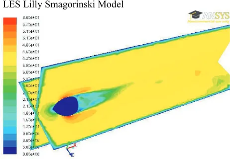
• LES Lilly Smagorinski Model

Figure 6. Instantaneous velocity field LES Lilly Smagorinski model

Figure 7. Time-averaging velocity field LES Lilly Smagorinski model

• LES WALE Model

Figure 8. Instantaneous velocity field LES - WALE model

Figure 9. Time-averaging velocity field LES - WALE model

From the comparison of the time-averaging velocity field and velocity field at any given time for each model: • Transition k-kl-omega – pulsations are detected in the X direction, but the actual modelling of vortices is not captured; wake behind the object is the smallest of the three turbulence models;

Furthermore, it is possible to graphically compare the pathlines for each turbulence models, velocity u = 100 m s-1:

• Transition k-kl-omega model

Figure 10. Pathlines Transition k-kl-omega model

• LES Lilly Smagorinski model

Figure 11. Pathlines LES Lilly Smagorinski model

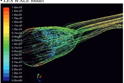
• LES WALE model

Figure 12. Pathlines LES WALE model

The figures (Figure 10-12) illustrate the flow shown by pathlines showing the instantaneous velocity at time 0.6144 s. From the comparison of pathlines for different turbulence models we can see strong swirl at LES models, especially LES WALE model. Transition turbulence model k-kl-omega model reveals a slight reverse swirl, wrap right behind the sphere which is flown around. With the increasing distance behind the ball the flow seem free of any swirl. LES models better

capture the pulsation and private swirl flow, appearing while wrapping of the obstacle. For model LES WALE area affecting the flow field barrier is appears greater than that of the model LES Lilly Smagorinski. We can identify a large swirl area swirl large area in the near distance for flow around body and then drift of the modelled vortices.

7 Final evaluations

In this paper, a comparison of three turbulent models for calculation of complex aerodynamic problems was made. These models were:

• Transition k-kl-omega model • LES Lilly Smagorinski model, • LES WALE model.

Aerodynamic task consisted of comparison of the drag coefficient Cd depending on the value of the

Reynolds number, for the flow around object - a sphere, obtained by finite volume method with the values reported in the literatures. We were also compared Strouhal number, also depending on the Reynolds number, for a given speed, obtained from experimental measurements and numerical data.

Comparison of the drag coefficient is performed in Graph 1. We can declare that the best results are acquired from the LES Lilly Smagorinski model, LES WALE model placed second in the preference and the Transition k-kl-omega model is the last.

The results of numerical modelling Strouhal numbers are listed in Table 5. By comparing the value StMEAS (17)

it can be concluded that the Strouhal number for a given speed, u = 10 m s-1 was assessed with the highest accuracy by the LES Lilly Smagorinski model, then by the LES WALE model, and finally by the Transition k-kl-omega model again.

The exact description of the turbulent flow field model is needed to define the source field for solving acoustic wave propagation in a given environment.

References

1. Bird, B. R., Warren, E. S. Transport Phenomena, 914 (2002)

2. Constantinescu, G. Numerical investigations of flow over a sphere in the subcritical and supercritical regimes, 18 (2004)

3. Dobeš, J. Kozubková, M. Modelování aerodyne-mického odporového souþinitele, 4 (SKMTaT, 2013) 4. Janalík, J. Obtékání a odpor tČles 43 (2002)

5. Kozubková, M. Drábková, S. ŠĢáva, P. Matematické modely nestlaþitelného a stlaþitelného proudČní, 112 (1999)

6. Ansys, Inc. ANSYS FLUENT V14.0 – Theory Guide, 826 (2011)

7. Dantec Dynamics. Probes for Hot-wire anemometry, 25.

8. Turbulence intensity, CFD ONLINE.