Simulation of the Propeller Disk Inside the Symmetrical Channel
Martin Kyncl1,aand Jaroslav Pelant1,b
1V´yzkumn´y a Zkuˇsebn´ı Leteck´y ´Ustav, a.s., VZL ´U, Beranov´ych 130, 199 05 Praha - Letˇnany, Czech Republic
Abstract. We work with the system of equations describing non-stationary compressible turbulent fluid flow, and we focus on the numerical solution of these equations, and on the boundary conditions. The computational simulation of the propeller disk is a demanding and time-consuming task. Here the propeller disk is represented by the distribution of the vector of velocities along its radius. The main purpose is to describe the special com-patible conditions used to simulate the propeller disk on the both its sides. In order to construct these conditions we analyze the equations in the close vicinity of the boundary. We use the analysis of the exact solution of the Riemann problem in order to solve this local boundary problem. The one-side modification of this problem has to be complemented with some other conditions. At the back side of the propeller disk, it is advantageous to use total density and the total pressure distribution, coming from the known distribution of axial velocities on the disk and the total state values at the inlet, and extra added velocities of rotation. At the front side of the disk, it is preferable to use the distribution of the flowing mass, known from the state values computed on the back side of the disk. We analyze the solution of these particular problems. We show the computational results of the flow around such propeller disk, obtained with the own-developed code for the solution of the 3D axis-symmetrical compressible turbulent gas flow.
1 Introduction
The numerical simulation of the propeller disk is always a difficult, and time-demanding task. For the proper simula-tion it is usually needed to work in 3D, using some sofisti-cated meshes. In this paper we work with the simple rotor, represented by the distribution of the velocity. Furthermore we assume the problem to be axis-symmetrical. We simu-late this rotor with the use of two connected boundaries. At these boundaries we solve the conservation laws, using the modification of the Riemann problem by the preference of the total quantities at the inlet, and the modification by the preference of the mass flow at the outlet. Numerical example of this approach is shown. In our simulation we consider the Reynolds- Averaged Navier-Stokes equations with the k-ωmodel of turbulence, rewritten into the axis-symmetrical form.
2 Formulation of the Equations
for an Axis-symmetrical Flow
For a symmetrical three dimensional flow we use the fol-lowing system of the equations
∂ ∂tq+
∂ ∂xf(q)+
∂ ∂yg(q)−
∂ ∂xr(q)+
∂ ∂ys(q)
=−1yF(q)+1
yG(q)
(1)
where
q=(, u, v, w,E)
f(q)=u, u2+p, uv, uw,(E+p)u a e-mail:[email protected]
b e-mail:[email protected]
g(q)=v, vu, v2+p, vw,(E+p)v
r(q)=0, τxx, τxy, τxz,
uτxx+vτxy+wτxz+γ(μ
Pr+ μT
PrT
)∂ε ∂x
s(q)=0, τxy, τyy, τzy,
uτxy+vτyy+wτzy+γ( μ
Pr + μT
PrT
)∂ε ∂y
F(q)=v, uv, (v2−w2),2vw,(E+p)v
G(q)=
0, μX
1 3
∂v ∂x+
∂u ∂y
, μX
4 3
∂v ∂y−
v y
, μX
∂w ∂y −
w y
,
μX
−4
3v ∂u ∂x+
1 3u
∂v ∂x+u
∂u ∂y−w
∂w ∂y
+
+γ( μ Pr +
μT
PrT
)∂ε ∂y−
2k 3 v
withμX=μ+μT,and
τxx=
+4
3 ∂u ∂x−
2 3
∂v ∂y
μX−
2k 3 τyy=
−2
3 ∂u ∂x+
4 3
∂v ∂y
μX−
2k 3 τxy=τyx=
∂v ∂x+
∂u ∂y
μX
τxz=
∂w ∂x
μX, τyz=
∂w ∂y
μX.
Herepis the pressure,the density, (u, v, w) is the av-erage value vector of velocity:uis the velocity in the direc-tionx, the componentsv,ware radial and circle velocities, DOI: 10.1051/
C
Owned by the authors, published by EDP Sciences, 2014 /2 01
x, y,zdenote the cylindrical coordinates: ydenote the ra-dius,zthe angle of rotation, andtthe time. Further,kis the turbulent kinetic energy of flux components of the veloc-ity,ωis the specific turbulent dissipation,Pris laminar and
PrT is turbulent Prandtl constant number,μis the dynamic
viscosity coefficient dependent on temperature,μT =k/ω
is the eddy-viscosity coefficient. In the energy equation,E denotes the total energy
E=ε+1 2(u
2+v2+w2),
whereε = p/(γ−1) is the internal energy of a unit mass of the fluid where the constantγ >1. This system of equations (1) is an open system for turbulent flow. The sys-tem studied (1) can be rewritten into the differential sym-bolic form
∂αi
∂t + ∂βi
∂x + ∂γi
∂y = fi
and in the integral form it reads
∂Ω((αi, βi, γi),n) ds=
Ω fi(x, y,t) dxdydt, (2) wherei = 1,2,3,4,5, Ωis from the spaceR3(t,x, y), and (,) denotes the scalar product.nis a normal vector to∂Ω. The positive orientation is given by the outward direction. Heresis the integral measure in the surface∂Ω. Using the integral form we can study a flow with shock waves, too.
3 Modification of the k -
ω
Standard
Turbulence Model for Axis-symmetrical
Flow
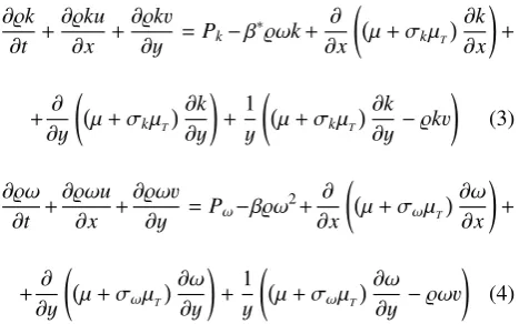
Turbulent model is described by following equations ∂k
∂t + ∂ku
∂x + ∂kv
∂y =Pk−β∗ωk+ ∂
∂x
μ+σkμT
∂k ∂x
+
+∂ ∂y
μ+σkμT
∂k ∂y
+1 y
μ+σkμT
∂k ∂y−kv
(3)
∂ω ∂t +
∂ωu
∂x +
∂ωv
∂y =Pω−βω2+ ∂ ∂x
μ+σωμT
∂ω ∂x
+
+∂y∂
μ+σωμT
∂ω ∂y
+1y
μ+σωμT
∂ω
∂y −ωv
(4) wherekthe turbulent kinetic energy andω the turbulent dissipation are functions of timet and space coordinates x, y. The production termsPkandPωare given by formulas
Pk=τxx∂
u ∂x+τxy
∂u
∂y+τyx∂∂v
x+τyy ∂v ∂y+
+μT
⎡ ⎢⎢⎢⎢⎢ ⎣
∂w ∂y
2 −4
3 ∂v ∂y v y−2
∂w ∂y
w y+
+4
3
v y
2
+
w y
2 −4
3 ∂u ∂x v y +
∂w ∂x
2⎤ ⎥⎥⎥⎥⎥
⎦−23ykv,
Pω= αωωPk
k , where αω= β β∗ −
σωκ˜2 √
β∗.
Here functions τ are defined in Sect. 2. for μ = 0, and σk,β∗,β,σω,κ˜are given constants, see [1]. This turbulent
modelk-ω(3), (4) with equations (1) presented the closed system of equations.
4 1D Riemann Problem for the Euler
Equations
We are concerned with one-dimensional Euler equations. ∂q
∂t + ∂f(q)
∂x =0, inQ∞=(−∞,+∞)×(0,+∞) (5) with notationq=(, u,E)T, f(q)=(u, u2+p,(E+ p)u)T.We assume equation of state for ideal gas holds
p=(γ−1)(E−u2/2) inQ∞.
u denotes velocity,density, p pressure.E denotes total energy. The system is hyperbolic. The Riemann problem for hyperbolic system (5) consists in finding its entropy weak solutioninQ∞, which satisfies the initial condition formed by two known constant statesqL, qR
q(x,0)=qL=(L, LuL,EL)T, x<0, (6)
q(x,0)=qR=(R, RuR,ER)T, x>0. (7)
The physical analogue to this problem is so-called shock-tube problem.
The general theorem on the solvability of the Riemann problem can be found in [4, page 88]. The solution q =
q(x,t) of Riemann problem (5),(6),(7) is piecewisesmooth
and its general form can be seen from figure 1, where a sys-tem of half lines is drawn. These half lines define regions,
-6t
x
0
@ @ @ @ @ @
l l l l l l l l
,, ,,
,, ,,
x
t=sHL sTL=xt xt=u xt=sTR sHR=xt
ΩHTL ΩL
ΩL ΩR
ΩR
ΩHTR
Fig. 1. Structure of the solution of the Riemann problem (5),(6),(7)
whereqis either constant or smooth. Let us define the open sets calledwedges(see figure 1):
ΩL=wedge(L−∞,sHL),
ΩHTL=wedge(sHL,sTL), ΩL=wedge(sTL,u∗),
ΩR =wedge(u,sTR),
ΩHTR=wedge(sTR,sHR), ΩR =wedge(sHR,L+∞).
The solution inΩL, ΩL, ΩR, ΩRis constant (see e.g. [4,
page 128])
q|ΩL =qL, q|ΩL =qL,
q|ΩR =qR, q|ΩR =qR.
1-shock wave, or 1-rarefaction wave). There is acontact discontinuity in between regions ΩL and ΩR. Wedges
ΩR andΩR are separated by right wave (either 3-shock
wave, or 3-rarefaction wave). Therefore there are four pos-sible wave patterns in the solution.
– Contact DiscontinuityPressurepand velocityudon’t change acrosscontact discontinuity, which separates ΩL andΩR region in general, and moving at speed
u
p|ΩL∪ΩR =p,
u|ΩL∪ΩR =u,
In general, there is a discontinuity in densityacross half line xt =u
|ΩL |ΩR in general.
It is clear, that there must be a jump in temperature, if there is a jump in density, but not in pressure. There is also a jump in entropy. Contact discontinuity is some-times calledentropy wave. In reality, contact disconti-nuities are smeared out due to diffusive effects, which are neglected and not included in hyperbolic system (5).
It is more convenient to use the vector of primitive vari-ables rather then the vector of conservative varivari-ables in solving the Riemann problem. We can denote these vec-tors of primitive variables in particular regions as
(,u,p)|ΩL =(L,uL,pL),
(,u,p)|ΩL =(L,u,p),
(,u,p)|ΩR=(R,u,p),
(,u,p)|ΩR=(R,uR,pR).
Here we show the equations for the primitive variables inΩL∪ΩHT L∪ΩL. For the solution of the whole system
see [4].
– 1-shock wave
One of the possible wave patterns connectingΩL and
ΩL is a shock wave. RegionΩHT L degenerates into
single half-line. Primitive variables,u,p“jump“ ac-cross this wave. It isu <uL,p >pL. Inviscid shock
jump relations can be derived, we call them
Rankine-Hugoniot relations. These leads us to following rela-tions across the 1-shock wave (see 4, or [4, page 125])
u=uL−(p−pL)
⎛ ⎜⎜⎜⎜⎜ ⎜⎝
2 (γ+1)L
p+γγ−+11pL
⎞ ⎟⎟⎟⎟⎟ ⎟⎠ 1 2
(8)
L=L
γ−1 γ+1
pL
p +1
pL
p + γ−1 γ+1
(9)
s1=uL−aL
γ+1 2γ
p pL +
γ−1
2γ , (10)
s1denotes speed of the 1-shock wave. Half line xt =s1 shapes the boundary between ΩL andΩL. It can be
shown (see [3]), that (8) can be rewritten in the form p=E1Ls(u), (11)
where
E1Ls(u)=pL+γ+
1
4 L(uL−u)
2+ (12)
+(uL−u)
2
4LγpL+
γ+1 2
2
2
L(uL−u)2,
andu<uL.
– 1-rarefaction wave
Another possible left wave pattern israrefaction wave. It formsΩHT Lregion.Variables changes smoothly within
this wave. Across the 1-rarefaction wavep≤pL,u≥ uL. Following equations are true.
u=uL+
2 γ−1aL
⎡ ⎢⎢⎢⎢⎢ ⎣1−
p pL
(γ−1)/2γ⎤ ⎥⎥⎥⎥⎥
⎦ (13)
L=L
p pL
1 γ
(14)
sT L=u−aL
p pL
(γ−1)/2γ
. (15)
HereaL=
γpL
ρL is the speed of sound in theΩL.sT L
is speed of the tail of the 1-rarefaction wave. Speed of the head of the rarefaction wave can be expressed
sHL=uL−aL. (16)
Half line xt = sT L shapes the boundary between ΩL
andΩHT L. Pressure positivity in (13) gives condition
u < uL+ γ2−1aL. Equation (13) can be written in the
form
p=pL
⎛ ⎜⎜⎜⎜⎜
⎜⎝−u+uL+ 2 γ−1aL 2
γ−1aL ⎞ ⎟⎟⎟⎟⎟ ⎟⎠ 2γ γ−1
. (17)
State variables inΩHT Lchanges continuously, and can
be expressed using equations (see [4], (3.1.97), page 118.)
(x,t)=L
2 γ+1+
γ−1 (γ+1)aL
uL−
x t
2 γ−1
, (18)
u(x,t)= 2 γ+1
aL+γ−
1 2 uL+
x t
, (19)
p(x,t)=pL
2 γ+1+
γ−1 (γ+1)aL
uL−
x t
2γ γ−1
. (20)
We combine both possibilities (11), (17) and we get equation for pressure pusing valuesL,uL,pL
p= ⎧⎪⎪⎪ ⎪⎪⎨ ⎪⎪⎪⎪⎪ ⎩
2pL+γ+1
2 L(uL−u)2+(uL−u)2
4LγpL+2L(γ+
1 2 )2(uL−u)2
2 , u<uL
pL
−u+uL+ 2 γ−1aL
2 γ−1aL
2γ γ−1
, uL≤u<uL+γ−21aL.
(21) Combining (9) and (14) we get equation for densityL
and pressurep
L=
⎧⎪⎪ ⎪⎪⎨ ⎪⎪⎪⎪⎩L
γ−1 γ+1pLp+1
pL p+γγ−1+1
, p>pL
L
p
pL
1 γ, p
≤pL.
Let us denotesL?the “wave speed” as follows:
sL?= !
s1, p>pL
sT L,p≤pL.
In case of 1-shock wave it denotess1 wave speed, in the case of 1-rarefaction wave it is the speed of the tail of the wavesT L. We combine (10) and (15) to obtain relation
be-tweensL?andp:
sL?= ⎧⎪⎪⎪ ⎨ ⎪⎪⎪⎩uL−aL
γ+1
2γ ppL +
γ−1
2γ ,p>pL
u−aL
p
pL
(γ−1)/2γ
, p≤pL.
(23)
There are four unknowns inΩLto resolve in order to get
the solution across left wave and the position of this wave. Relations of these unknownsL,p,uand the wave speed
sL?to left state variablesL,uL,pLare given by three
equa-tions (21),(22),(23). To get state variables across left wave, i.e. inΩL∪ΩS T L∪ΩL, and position of the wave, we have to
add another equation into the system (21),(22),(23). There is a jump in density across contact discontinuity. This brings another unknownRto unknownsL,p,u,sL?. We have to add two properly chosen equations into this system of equations in order to get uniquely solvable system for 5 unknowns sought inΩL∪ΩS T L∪ΩL∪ΩRregion.
5 Boundary Condition by the Preference of
Total Pressure and Total Density
In this section we will analyze the initial-boundary value problem formed by the Euler equations (5), equipped with the left-hand side initial condition (6) and the complemen-tary conditionsgiven as
p=po
⎛
⎜⎜⎜⎜⎝1−γ−1 2a2
0 u2
⎞ ⎟⎟⎟⎟⎠γ/(γ−1)
, (24)
θR=θo
1−γ−1 2a2
o
u2
, (25)
u<0. (26)
Hereθo > 0,po > 0 are given constants anda2o = γRθo.
FurtherRdenotes the characteristic gas constant, andγis the adiabatic constant. The equations (24),(25) are consid-ered for the velocityu ∈
− 2a2
o
(γ−1),
2a2
o
(γ−1)
. Using (26), the interval of interest is
−
2a2
o
(γ−1) <u<0. (27) The equations (25),(24) come from the idea, that the total pressure po and thetotal temperatureθo are known
(prescribed) in the regionΩR.Theboundary stateqBis
the solution of the system (5),(6),(24),(25) at the half line SB = {( ˜x1,t); ˜x1=sB t; t>0}, sB = 0. At first, we
re-solve the velocityuin theStar RegionΩR∪ΩL,
intro-duced in Section 4.
Solution for the velocityu The condition (24) has the form
p=Epo(u), (28)
whereEpo(u)=po
1−γ2−a12
ou
2 γ/(γ−1).We will use the anal-ysis in Section 4, and discuss the condition (28) together with the equation for the pressure (21) and the condition (26). We get the velocityusolving the equation
F(u)=0, (29)
where
F(u)=Epo(u)−
!
E1Ls(u),uL>u,
E1Lr(u),uL≤u<uL+γ2−1aL,
−
2a2
o
(γ−1) <u<0.
HereaL denotes the speed of sound inΩL, the functions
E1Ls(u) and E1Lr(u) are defined in (11),(17). We seek the
velocityuin the interval (27).
There is no admissible solution of the system (5),(6), (24), (25) if uL+ γ−21aL < −
2a2
o
(γ−1), the extreme value yields the zero pressure p =0.In practical applications, we may prescribe the closest velocityu =−
2a2
o
(γ−1) +, with >0 being a small positive constant, though it is not the solution of the system.
Let us analyze the functionF(u) for the 1-shock and for the 1-rarefaction wave separately.
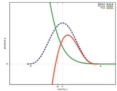
Fig. 2.Example of the functionsEpo(u),E1L(u),F(u) for the
ini-tial datapo=101325, θo =273.15,pL=70000, L=1.25,uL=
−100.HereA=
2a2
o
(γ−1).
1-shock wave
For the 1-shock wave it is u < uL. Using the function
for the pressure (11), we write
F(u)=po
1−γ−1 2a2
o
u2 γ/(γ−1)
−pL−γ+
1
4 L(uL−u) 2
−(uL−u)
2 "
4LγpL+2L(γ+
1 2 )
2(u
considered for
u<uL,−
2a2
o
(γ−1) <u<0.
We cannot use the form (30) in the case ofuL≤ −
2a2
o
(γ−1), as u < uL for the 1-shock wave. The formulation (30)
makes sense also foru∈ {uL,0}. If−
2a2
o
(γ−1) <uLthen we seek the root of (30) in the interval (−
2a2
o
(γ−1),min{uL,0}). It holdsF(u)>0 in this interval, andF(−
2a2
o
(γ−1))<0.If F(min{uL,0})>0, then the solutionuis unique.
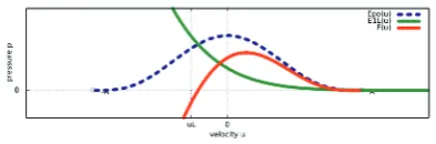
Fig. 3.Example of the functionsEpo(u),E1L(u),F(u) for the
ini-tial datapo =101325, θo=273.15,pL=70000, L=1.25,uL=
40.In this example the problem (29) has one solution with the 1-shock wave. It isu<0.
1-rarefaction wave
ForuL ≤u <uL+γ−21aLwe use the velocity function for
the 1-rarefaction wave, defined in (17). Let us find the root of the functionF(u)=Epo(u)−E1Lr(u). It is
F(u)=po
1−γ−1 2a2
o
u2 γ/(γ−1)
−pL
⎛ ⎜⎜⎜⎜⎜
⎜⎝uL−u+ 2 γ−1aL 2 γ−1aL
⎞ ⎟⎟⎟⎟⎟ ⎟⎠ 2γ γ−1 ,
(31) in the interval of interest
uL≤u<uL+
2
γ−1aL, −
2a2
o
(γ−1) <u<0. ForuL>0 there is no solution with the 1-rarefaction wave.
IfF(max{uL,−
2a2
o
(γ−1)})<0 andF(min{0,uL+ 2 γ−1aL})> 0, then there is a unique root of the function (31), see [3]. It is
u= 2
uL+γ−21aL −
√ DIS
2 #
1+ 2a2L
(γ−1)a2
o
p
o
pL
(γ−1)/γ$, (32)
DIS=4
po pL
(γ−1)/γ 2a2
L
(γ−1)a2o ⎡ ⎢⎢⎢⎢⎢ ⎢⎢⎣ 2a2o
(γ−1)+ 4a2
L
(γ−1)2
po pL
(γ−1)/γ −
uL+γ2aL−1
2⎤⎥⎥⎥⎥⎥
⎥⎥⎦.
Fig. 4.Example of the functionsEpo(u),E1L(u),F(u) for the
ini-tial datapo=101325, θo=273.15,pL=100000, L=1.25,uL=
−200.In this example the problem (29) has one solution with the 1-rarefaction wave.
Summarizing the above possibilities of the 1-shock and the 1-rarefaction wave we can construct the algorithm in figure 5 for the computation of the velocityu in thestar region.
The problem (29) has a unique solution for the initial data satisfying
uL+
2
γ−1aL>−
2a2
o
(γ−1), F(min{0,uL+ 2
γ−1aL})>0. (33) In the case ofuL+γ−21aL ≤ −
2a2
o
(γ−1) there is no solution of the system (5),(6),(24),(25) with (26). In this case we prescribe the velocityu=−
2a2
o
(γ−1)+,with >0 being a small positive constant. If F(min{0,uL + γ−21aL}) ≤ 0
then the problem (29) does not have a negative solution, and for the practical applications we choose the velocity u=min{0,uL+γ2−1aL}.
-yes
uL≥0
?
no
F(0)≥0 yes- u=root of (30)
?no
Failed, chooseu=min{0,uL+γ−21aL}
uL+γ−21aL>−
2a2
o
(γ−1) yes- F(min{0,uL+ 2
γ−1aL})<0 6yes
?no ?no
Failed, choose
u=−
2a2
o
(γ−1)+
− 2a2
o
(γ−1) ≥uL yes- use (32)
?no
F(uL)<0 yes- use (32)
?no
u=root of (30)
Fig. 5.Algorithm for the velocity solutionu<0 of the problem (29). In the case of failure, the problem doesn’t have a solution, and the values are chosen.
Solution inΩL∪ΩHT L∪ΩL∪ΩR
Knowing the velocityu we compute the pressurep us-ing (28), and the density L using (22) uniquely. In the
case of the 1-rarefaction wave, the solution inΩHT Lis
com-puted using the equations (18), (19), (20). At last we are interested in the densityR. The equation of state holds
in the regionΩ∗R
R=
Further we use the equation for thetotal temperature(25) and the equation (28). We write
R=
p RθR =o
1−γ−1 2a2
o
u2
1/(γ−1)
. (34)
Hereo= Rpθoo denotes thetotal densityinΩR.
Solution in(−∞,∞)×(0,∞)
At first we compute the solution inΩL∪ΩHT L∪ΩL∪
ΩR, as shown in 5. Further we add thecomplementary
condition
pR=p. (35)
Then it isu =uR,andR =R, see [3].u =uR,and
R =R. This way the prescribedtotal pressureandtotal
temperatureare preferred also inΩRregion.
The complementary conditions (24),(25),(35) with (26) yield the well-posedinletboundary condition for the sys-tem (5),(6) only if (33) is satisfied. If (33) is not satisfied, then thetotal quantitiescannot be preferred at the bound-ary. In the practical application we prescribe the closest ad-missible value for the velocityuand compute the bound-ary state accordingly, or we use the boundbound-ary condition preferring the static pressure p = po, see [2, 3], in this
case.
5.1 Boundary Condition by the Preference of Mass Flow
In this section, we attempt to solve the incomplete modi-fied Riemann problem for the Euler equations (5),(6), seek-ing the solution in the general form of the Riemann prob-lem solution, consisting of 4 constant states separated by 3 waves. VariablesL,uL,pLare known from the initial
con-dition, also the speed of soundaL is known. We add the
boundary condition for the mass flow inΩLgiven as
uL=G, (36)
whereG ≥ 0 is given constant (G = mass f lof ace areaw). Here u, L denotes unknown parts of the solution in the
re-gionΩL.Velocityu(x,t) and density(x,t) are constant
in this region, as was mentioned in 4.
Here we note, that the system (5),(6),(36) may not have any solution for a givenG or it may have multiple solu-tions for the certain choice ofG. In this article we will prefer the solutions with the left rarefaction wave. We will transfer the problem (5),(6),(36) into the boundary prob-lem described in [2] with the velocityugiven. It is basi-cally the use of the equations (8),(9),(10), or (13),(14),(15) for known u.If G = 0, then apparently u = 0, and we may use the analysis for the boundary condition by the preference of velocity shown in [2].
– 1-rarefaction wave
Here we will try to find the primitive variablesL,u, psuch that (13),(14),(36) wihuL ≤u <uL+γ2−aL1 is
satisfied. From (13),(14),(36) it is
uL
1−γ−1 2aL
(u−uL)
2 γ−1
−G=0. (37)
We find the velocityuas the root of the functionF(u)= uL
1−γ2−a1
L(u−uL)
2 γ−1 −
G on the appropriate in-terval. Then the unknownsL,pare evaulated from (13), (14). It isF(0)=F(uL+γ2−aL1)<0. The first
deriva-tive F(u) = L
1−γ2−a1
L(u−uL)
2 γ−1#
1− u
aL−γ−12 (u−uL)
$
is zero at the pointsu0 = γγ−+11
uL+γ2−aL1 , u1 = uL+
2aL
γ−1. Derivative F(u) > 0 in the interval (0,u0) and F(u)<0 foru ∈(u0,u1).The maximum of the func-tionF is at the pointu0. The problem of the existence of the roots depends on the sign of F(max(uL,u0)). If F(max(uL,u0)) ≥ 0 then there exists such u sat-isfying (37), and the problem (5),(6),(36) has a solu-tion with 1-rarefacsolu-tion wave. IfuL < u0 andF(uL) ≤
0, F(u0)>0 then the problem (37) has two solutions, and we choose the smaller one. There is no solution if F(max(uL,u0))<0.
LetuL < 0. In the case of 1-shock wave it is u < uL, uL < 0, and (36) cannot be satified. Therefore
the solution with 1-rarefaction wave is the only solution possible anducan be found as the solution of the (37). If F(u0)<0 then the problem doesn’t have any solution and one may choose the solution withu=u0as this gives the mass flow closest toGforuL<0.
LetuL≥0. IfF(max(uL,u0))≥0 then there exists a so-lution of the problem (5),(6), (36) with 1-rarefaction wave. With the velocity u known, we use the analysis for the boundary condition by the preference of velocity shown in [2].
If F(max(uL,u0)) < 0 then there is no solution with 1-rarefaction wave andLuL−G < 0.We will show that for LuL−G < 0,uL < aL there is no solution with
1-shock wave either. ForuL<aLit is s1<0.The Rankine-Hugoniot condition hold across 1-shock wave (see [4, page 120 (3.1.109)])L(uL−s1)=L(u−s1).It isL< Lfor
1-shock and thereforeLuL−G=s1(L−L)<0.This is
in contradiction withLuL−G>0. In the case ofuL<aL
there is no solution with the 1-rarefaction nor the 1-shock wave. We chooseu=max(u0,uL). In the case ofuL>aL
the solution may not exist, though for an existing solution it iss1>0 orsHL>0. We choose (B,uB,pB)=(L,uL,pL)
at the boundary in this case.
6 Examples
Here we present the computational simulation of the pro-peller disk by a given velocity profile. The computational results are shown in figure 6 and figure 7. The results were obtained with the own-developed codes (the RANS with the k-w model of turbulence). The gas constants for the air are κ = 1.4 andR = 287.04 J kg−1 K−1. We use the viscosity coefficient (depending on the local temperature) computed with the use of the Sutherland’s law
μ=μre f
T Tre f
3/2
Tre f +S
T +S ,
withS = 110.4 K,Tre f =273.15 K,μre f = 1.716e−05
– geometry - the given geometry is shown in figure 6.
– initial condition - constant state in the whole domain, To=273.15 K,u=(0,0,0), po=101325 Pa.
– inlet boundary condition (left) - total quantities and zero tangential velocity (no rotation at the inlet). This boundary condition was described in Sect. 5, total pres-surepo=101325 Pa, total temperatureTo=273.15 K,
and zero tangential velocity (v=0 m s−1).
– outlet boundary condition (right) - preference of the pressure, shown in [2, 3]. Given pressurep=101325 Pa was used.
– wall boundary condition (up, bottom) - preference of the velocity, shown in [2, 3]. Zero velocity at the wall was given together with the wall temperatureTW ALL =
273.15 K.
– the propeller disk:
– back side: the total density and the total pressure distribution, and the given velocity of the rotation (tangential components). Here the total pressurepDo
and the total densityDo (at the given point) are
given (constant in time) as
pDo=po
1+κ−1
2 M
2 κ
κ−1
Do=o
1+κ−1
2 M
2 1
κ−1
HereM2 =v2
ax/(κRTo) andvax is the axial
compo-nent of the velocity at the given point andpo,Toare
the values from the inlet boundary condition.
– front side: the preference of the mass flow, values computed from the back side of the disk.
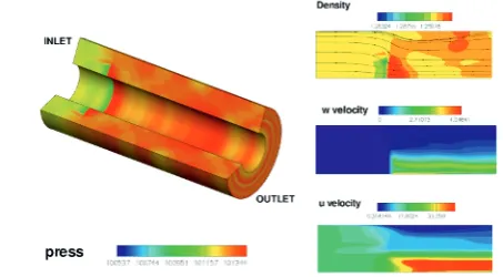
Fig. 6.The propeller disk simulation, computational mesh con-sisted of 211x95 elements (left). Red line represents the propeller disk.
Fig. 7.Compressible gas flow through the propeller disk, the pressure isolines, the density isolines, the radial and the axial ve-locity components in the meridian plane.
Conclusion
This paper shows the analysis of the boundary condition for the simulation of the propeller disk by the given veloc-ity profile. This procedure is then used in the finite volume method for the simulation of the propeller placed in the three-dimensional axis-symmetrical channel.
Acknowledgment
This result originated with the support of Ministry of In-dustry and Trade of Czech Republic for the long-term strate-gic development of the research organisation. The authors acknowledge this support.
References
1. C. J. Kok. AIAA Journal, Vol.38., No. 7., (2000). 2. M. Kyncl and J. Pelant. Applications of the
Navier-Stokes equations for 3d viscous laminar flow for symmet-ric inlet and outlet parts of turbine engines with the use of various boundary conditions.Technical report R3998, VZL ´U, Beranov´ych 130, Prague, (2006).
3. M. Kyncl. Numerical solution of the three-dimensional compressible flow.Master’s thesis, Prague, (2011). Doc-toral Thesis.