FULL PAPER
Improvements and validation of the IRI
UP method under moderate, strong, and severe
geomagnetic storms
Alessio Pignalberi
1*, Marco Pietrella
2, Michael Pezzopane
2and Rolando Rizzi
1Abstract
This work describes several important improvements made to the International Reference Ionosphere UPdate (IRI UP) method, and a careful validation of its performances under disturbed conditions. The IRI UP method has been improved developing an algorithm capable to properly filter wrongly autoscaled ionosonde data to be assimilated, avoiding the use of these in the assimilation process. Furthermore, the preliminary quality check used to choose the variogram model in the Universal Kriging method has been replaced with a new quality check routine (NQCR), based on statistical tests carried out using the variables Q1, Q2, and cR, built on variogram’s residuals. NQCR objectively identi-fies the best variogram model from which to get more reliable effective indices maps to be ingested in the IRI model to obtain updated foF2 and hmF2 maps. IRI UP has been applied on 30 different time intervals, between January 1, 2004, and December 31, 2016, characterized by moderate, strong, and severe geomagnetic conditions, over the European region. A statistical comparison between IRI UP and IRI at the truth sites located at Fairford (51.7°N, 1.5°W, UK) and San Vito (40.6°N, 17.8°E, Italy), for foF2 and hmF2, has been performed. From the statistical validation clearly emerges how IRI UP, for foF2, performs significantly better than IRI, for each of the 30 geomagnetic storms considered. Regarding hmF2, IRI UP performances are lower than those for foF2, although still better than IRI ones. In the light of the results achieved in this investigation, the IRI UP method represents an interesting approach to Space Weather forecast in the ionospheric domain.
Keywords: IRI UP, Universal Kriging, Ionospheric data assimilation, Nowcasting maps
© The Author(s) 2018. This article is distributed under the terms of the Creative Commons Attribution 4.0 International License (http://creat iveco mmons .org/licen ses/by/4.0/), which permits unrestricted use, distribution, and reproduction in any medium, provided you give appropriate credit to the original author(s) and the source, provide a link to the Creative Commons license, and indicate if changes were made.
Introduction
Space Weather events can significantly affect the func-tioning of radio systems, with effects that can be rapid (immediately after the event) or delayed (a few days after the event). High-frequency (HF) point-to-point com-munications exploit the terrestrial ionosphere and rep-resent a valid and complementary alternative to satellite communications. The ionosphere is a complex dynamic propagation environment, and this makes HF commu-nications problematic even during not so intense Space Weather events, because of its intrinsic variability (e.g., Kouris et al. 1998; Kouris and Fotiadis 2002). Extreme
events occurring on the Sun, such as flares and coronal mass ejections, produce important variations of the cor-puscular (solar wind) and electromagnetic [ultraviolet (UV) and X-ray emissions] component arriving on the Earth, which have a deep impact on the magnetosphere– ionosphere–atmosphere system (Zolesi and Cander
2014). As a consequence of such events, under particu-lar conditions [i.e., when the north-south component Bz
of the Interplanetary Magnetic Field is orientated south-ward (Bz < 0)], moderate, strong, and severe geomagnetic storms can occur giving rise to ionospheric storms, since the dynamics and structure of the ionosphere are signifi-cantly affected by the geomagnetic activity (Buonsanto
1999). Under ionospheric storm conditions, empirical climatological models, like the International Reference Ionosphere (IRI) model (Bilitza et al. 2014, 2017; Bilitza and Reinisch 2008), are not able to properly predict the
Open Access
*Correspondence: [email protected]
1 Dipartimento di Fisica e Astronomia, Università di Bologna “Alma Mater Studiorum”, Bologna, Italy
ionospheric behavior, in particular during severe geo-magnetic storms, as recently demonstrated for instance by Pignalberi et al. (2016). Moreover, ionospheric storms give rise to an abnormal behavior of the HF operative band, with important repercussions on the reliability of radio communications at both regional and global scale. In these circumstances, in order to select the best fre-quencies to be used for HF communications, timely and accurate information about the ionospheric channel is required. That is why, as established by the IRI com-munity (Bilitza et al. 2011, 2014, 2017), real-time space-sparse ionosonde data should be used in conjunction with climatological models in order to get a picture of the ionospheric plasma variability as near as possible to the real conditions.
Currently, this is made possible thanks to the modern ionospheric stations which are equipped with software that provides, in almost real time, the electron den-sity profile and the ionospheric characteristics among which, from the radio propagative point of view, the most important are the critical frequency of the F2 ionospheric layer, foF2, and the propagation factor M(3000)F2.
Assimilating F2 layer characteristics and electron den-sity profiles, obtained from ionosonde measurements, into background ionospheric models, it was possible to develop nowcasting models which have been repeatedly proved to be effective in providing a better comprehen-sive specification of the ionosphere (Angling and Khatta-tov 2006; Thompson et al. 2006; Decker and McNamara
2007; McNamara et al. 2007, 2008, 2010, 2011; Nava et al.
2011; Shim et al. 2011; Galkin et al. 2012; Pezzopane et al.
2011, 2013; Pietrella 2015; Pignalberi et al. 2018a, b). Nowcasting models provide foF2, M(3000)F2, hmF2, and electron density maps, which have great value from the operative point of view, because their use is aimed at maximizing the reliability and availability of HF services, especially under very disturbed ionospheric conditions as those occurring during geomagnetic and ionospheric storms.
In the light of these considerations, it is easy to under-stand how important is to supply maps as reliable as possible. To this regard, a method, called International Reference Ionosphere UPdate (IRI UP), has been recently developed by Pignalberi et al. (2018a, b) as a valid alter-native to both the Simplified Ionospheric Regional Model UPdating (SIRMUP) model (Zolesi et al. 2004; Tsagouri et al. 2005) and the IRI-SIRMUP-P (ISP) model (Pezzo-pane et al. 2011, 2013).
The IRI UP method, which has the potentiality to work over any area where an appropriate number of autoscaled ionosonde measurements are available, assimilates ionosonde foF2 and M(3000)F2 data and, rely-ing on the Universal Krigrely-ing geostatistical interpolation
technique (Kitanidis 1997), produces maps of effective values IG12eff of the 12-months smoothed ionospheric index IG12 [derived by the IG index as calculated by Liu et al. (1983)], and maps of effective values R12eff of the 12-month smoothed sunspots number R12 (Houminer et al. 1993).
IG12eff and R12eff maps are then taken as input by the IRI climatological model to update the ionospheric back-ground, thus providing an instantaneous two-dimen-sional (2-D) mapping of foF2 and M(3000)F2 and, hence, of hmF2 in the region of application. Its validation was early conducted for a case study taking into account only the severe St. Patrick geomagnetic storm occurred on March 17, 2015 (Pignalberi et al. 2018a, b).
It must be kept in mind that the goodness of IRI UP nowcasting maps depends mainly on two important issues: (a) foF2 and M(3000)F2 data, autoscaled in some reference stations, constitute a discrete dataset which must be as reliable as possible because this dataset is used to compute the values of IG12eff and R12eff at each reference station; (b) the Kriging interpolation method which, starting from the discrete values of IG12eff and R12eff, provides IG12eff and R12eff nowcasting maps over the area under consideration, depends crucially on the choice of the variogram model which fits the experimental one. Therefore, in order to get a proper interpolation and con-sequently reliable IG12eff and R12eff maps, it is extremely important that selected variogram models have a good quality.
With regard to these two issues, in the work of Pignal-beri et al. (2018a, b), the reliability of foF2 and M(3000) F2 autoscaled data was based on a quality check of ionograms: for the reference stations equipped with the Automatic Real-Time Ionogram Scaler with True height analysis (ARTIST) software (Reinisch and Huang 1983; Reinisch et al. 2005; Galkin and Reinisch 2008), only ionograms with a Confidence Score (CS) greater than 75 (see http://www.ursi.org/files /Commi ssion Websi tes/ INAG/web-73/confi dence _score .pdf) were selected; for the reference stations equipped with the Autoscala soft-ware (Scotto and Pezzopane 2002, 2008; Pezzopane and Scotto 2005, 2007; Scotto 2009; Scotto et al. 2012), a care-ful visual inspection was adopted to select the reliable ionograms. Furthermore, to avoid unrealistic IG12eff and R12eff maps, a preliminary quality check of the variogram model, based on the exponent s of the power variogram model was also implemented.
2004, to December 31, 2016. The validation of the IRI UP method is carried out comparing the IRI UP perfor-mance with the one of the IRI model with the STORM option “ON,” at the two truth sites of Fairford (51.7°N, 1.5°W, UK) and San Vito (40.6°N, 17.8°E, Italy).
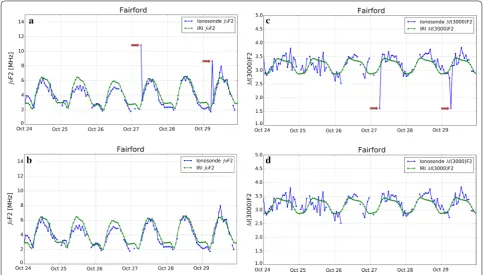
Moreover, an appropriate filter (F) was implemented in the IRI UP method to automatically discard those iono-sonde data clearly wrong (spikes) which, once assimi-lated, would affect negatively the ionospheric modeling. Its application turned out to be more effective than CS and visual inspection methods.
In addition, a new quality check routine (NQCR), based on statistical tests carried out using the statistical vari-ables Q1, Q2, and cR, built on the residuals [differences between the observed (experimental variogram) and the modeled (variogram model) semivariance values], has also been proposed with the intention of replacing the quality check based on the exponent s of the power vario-gram model. This allowed to select more objectively, and with a more acceptable degree of confidence, the “best” variogram model to be used.
The data used and periods under study are presented in “Data used and periods under study” section. The description of the F algorithm implemented in the IRI UP method is provided in “Description of the filter implemented to select ionosonde data” section. A recall to the Kriging interpolation method is outlined in “The Kriging interpolation method: a brief recall” section. The description of the NQCR procedure is provided in “On the choice of the best variogram model in the Uni-versal Kriging procedure: a new quality check routine (NQCR)” section. The validation of the IRI UP method and results obtained applying the NQCR procedure are the subject of “Validation of IRI UP method including the F algorithm and the NQCR procedure: some results” sec-tion. The discussion about the results and possible future developments is given in “Discussion, conclusions, and future developments” section.
Data used and periods under study
The data used in this study consist of: (a) Ap geomag-netic index data (Rostoker 1972); (b) Kp geomagnetic index data (Menvielle and Berthelier 1991); (c) foF2 and
M(3000)F2 data.
Geomagnetic indices were downloaded from the OMNIWeb Data Explorer—NASA site at https ://omniw eb.gsfc.nasa.gov/form/dx1.html.
foF2 and M(3000)F2 data were downloaded from the interactive ionogram scaling software, SAO Explorer, developed at the University of Massachusetts Lowell Center for Atmospheric Research (UMLCAR) (http:// ulcar .uml.edu/SAO-X/SAO-X.html) (Khmyrov et al.
2008; Reinisch and Galkin 2011).
In particular, foF2 and M(3000)F2 values from Rome and Gibilmanna were autoscaled from the ionograms recorded by an AIS-INGV ionosonde (Zuccheretti et al.
2003), and those from Warsaw were autoscaled from the ionograms recorded by a VISRC2 ionosonde (Pezzopane et al. 2009).
The ARTIST system was instead applied to autoscale
foF2 and M(3000)F2 data from the ionograms recorded by digisondes (Bibl and Reinisch 1978) installed in the remaining ionospheric stations.
Table 1 provides an overview of the ionospheric sta-tions considered, highlighting the ionosonde type, the autoscaling software, and the state of the station. The state “assimilated” means that foF2 and M(3000)F2 hourly values are assimilated to update the background model, while the state “used as test site” indicates that foF2 and
M(3000)F2 hourly values are used only to test the IRI UP performance. The ionospheric stations available for data assimilation are listed for each year in Table 2. Figure 1
shows the geographical distribution of the ionospheric stations under consideration.
The IRI UP performance was evaluated at the testing stations of Fairford and San Vito over 30 time intervals characterized by geomagnetic storms occurred between January 1, 2004, and December 31, 2016. Such period embraces part of the past 23rd solar cycle (August 1996– December 2008) and the current one. Ap daily mean values > 50 and Kp maximum values > 5+ (see https :// www.space weath erliv e.com/en/help/the-kp-index ), as recorded during the main phase day of the storm, are the thresholds adopted to discard minor storms, thus select-ing only the moderate, strong, and severe ones.
Specifically, each time interval was selected consider-ing the day before the main phase of the storm (which in the selected cases is always a quiet day), the day of the main phase, and the next 4 days of the recovery phase, for a total number of 6 days for each time interval. Nev-ertheless, when the storm is characterized by substorms with Ap daily mean > 50, then from the last substorm occurred, 4 days of the recovery phase are further con-sidered; this means that, in these cases, the period under study can be characterized by more than 6 days. Some information about the geomagnetic storms considered in this study is summarized in Table 3.
Description of the filter implemented to select ionosonde data
reliability of assimilated data; (b) to speed up the selec-tion process of data which are going to be assimilated.
The way the F algorithm works is as follows. In order to understand whether a value of foF2 or M(3000)F2 at a given hour hr [foF2hr and M(3000)F2hr, respectively] has been correctly autoscaled, foF2 and M(3000)F2 data, autoscaled in the previous 15 days at the same considered hour, are taken into account to calculate the mean val-ues m¯foF2,hr,15prevdays and m¯M(3000)F2,hr,15prevdays and the
corresponding standard deviations sdfoF2,hr,15predays and sdM(3000)F2,hr,15predays. Specifically, standard deviations are calculated when time series have a number N of available data greater than 5; otherwise, they are fixed to 0.5 MHz and 0.15 for foF2 and M(3000)F2, respectively.
Subsequently, if sdfoF2,hr,15predays ≥ 0.5 MHz, foF2hr is considered reliable if the following inequalities are fulfilled
otherwise, if sdfoF2,hr,15predays < 0.5 MHz, foF2hr is consid-ered reliable if the following inequalities are fulfilled
(1) ¯
mfoF2,hr,15prevdays−5sdfoF2,hr,15prevdays≤foF2hr
≤ ¯mfoF2,hr,15prevdays+5sdfoF2,hr,15prevdays;
(2) ¯
mfoF2,hr,15prevdays−5(0.5)≤foF2hr ≤ ¯mfoF2,hr,15prevdays+5(0.5). Table 1 European ionosonde network involved in the study
List of ionospheric stations considered in the study and their geographical coordinates. The ionosonde type, the autoscaling software, and the state of the station are also highlighted. In italics the stations used as test site
Ionospheric stations Lat (°) Lon (°) Ionosonde type Autoscaling software State
Athens (Ath) 38.0°N 23.5°E Digisonde DPS-4D ARTIST 5 Assimilated
Chilton (Chi) 51.5°N 0.6°W Digisonde DPS-1 ARTIST 4 Assimilated
Dourbes (Dou) 50.1°N 4.6°E Digisonde DPS-4D ARTIST 5 Assimilated
El Arenosillo (ElA) 37.1°N 6.7°W Digisonde DPS-4D ARTIST 5 Assimilated
Fairford (Fai) 51.7°N 1.5°W Digisonde DPS-4D ARTIST 5 Used as test site
Gibilmanna (Gib) 37.9°N 14.0°E AIS-INGV Autoscala 4.1 Assimilated
Juliusruh (Jul) 54.6°N 13.4°E Digisonde DPS-4D ARTIST 5 Assimilated
Moscow (Mos) 55.5°N 37.3°E Digisonde DPS-4 ARTIST 5 Assimilated
Nicosia (Nic) 35.0°N 33.2°E Digisonde DPS-4D ARTIST 5 Assimilated
Pruhonice (Pru) 50.0°N 14.6°E Digisonde DPS-4D ARTIST 5 Assimilated
Rome (Rom) 41.8°N 12.5°E AIS-INGV Autoscala 4.1 Assimilated
Roquetes (Roq) 40.8°N 0.5°E Digisonde DPS-4D ARTIST 5 Assimilated
San Vito (SaV) 40.6°N 17.8°E Digisonde DPS-4D ARTIST 5 Used as test site
Warsaw (War) 52.2°N 21.1°E VISRC2 Autoscala 4.1 Assimilated
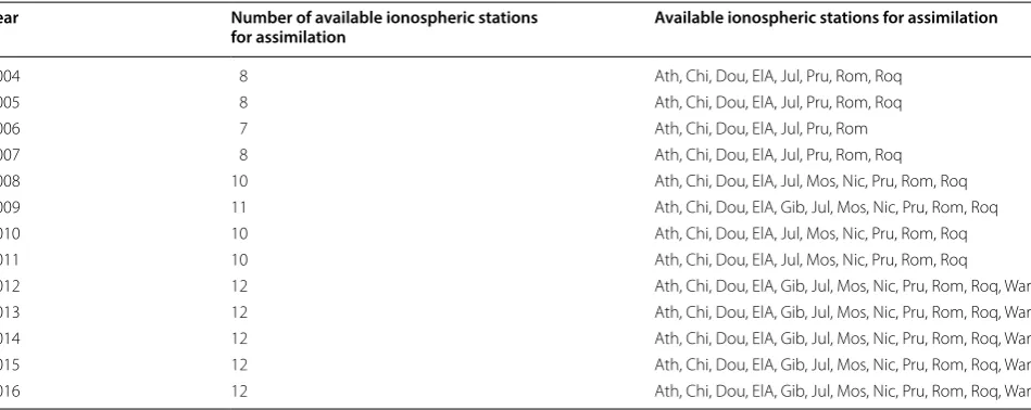
Table 2 Ionosonde stations temporal availability
Ionospheric stations available for data assimilation for each year, from 2004 to 2016
Year Number of available ionospheric stations
for assimilation Available ionospheric stations for assimilation
2004 8 Ath, Chi, Dou, ElA, Jul, Pru, Rom, Roq
2005 8 Ath, Chi, Dou, ElA, Jul, Pru, Rom, Roq
2006 7 Ath, Chi, Dou, ElA, Jul, Pru, Rom
2007 8 Ath, Chi, Dou, ElA, Jul, Pru, Rom, Roq
2008 10 Ath, Chi, Dou, ElA, Jul, Mos, Nic, Pru, Rom, Roq
2009 11 Ath, Chi, Dou, ElA, Gib, Jul, Mos, Nic, Pru, Rom, Roq
2010 10 Ath, Chi, Dou, ElA, Jul, Mos, Nic, Pru, Rom, Roq
2011 10 Ath, Chi, Dou, ElA, Jul, Mos, Nic, Pru, Rom, Roq
2012 12 Ath, Chi, Dou, ElA, Gib, Jul, Mos, Nic, Pru, Rom, Roq, War
2013 12 Ath, Chi, Dou, ElA, Gib, Jul, Mos, Nic, Pru, Rom, Roq, War
2014 12 Ath, Chi, Dou, ElA, Gib, Jul, Mos, Nic, Pru, Rom, Roq, War
2015 12 Ath, Chi, Dou, ElA, Gib, Jul, Mos, Nic, Pru, Rom, Roq, War
The inequalities (2) are considered because it may hap-pens that when very quiet days occur, the previous 15 days are characterized by foF2 values very close to each other; in these cases, the value of sdfoF2,hr,15predays would be too small and, consequently, the inequalities (1) would constitute a too selective filter.
The values of foF2hr considered reliable are then used to calculate IG12eff values at the hour hr in the correspond-ing assimilated ionosonde station (Pignalberi et al. 2018a,
b).
Likewise, if sdM(3000)F2,hr,15predays > 0.15, M(3000)F2hr is considered reliable if the following inequalities are fulfilled
otherwise, if sdM(3000)F2,hr,15predays < 0.15, M(3000)F2hr is considered reliable if the following inequalities are fulfilled
As already said for foF2, the inequalities (4) replace the inequalities (3) which would constitute a too selective filter.
The values of M(3000)F2hr considered reliable are then used to calculate R12eff at the hour hr (Pignalberi et al. 2018a, b).
The aim of the proposed F algorithm is to remove spikes, that is values of foF2 and M(3000)F2 which are
(3) ¯
mM(3000)F2,hr,15prevdays−5sdM(3000)F2,hr,15prevdays
≤M(3000)F2hr ≤ ¯mM(3000)F2,hr,15prevdays +5sdM(3000)F2,hr,15prevdays;
(4) ¯
mM(3000)F2,hr,15prevdays−5(0.15)≤foF2hr
≤ ¯mM(3000)F2,hr,15prevdays+5(0.15).
evidently wrongly autoscaled. Figure 2 shows an exam-ple of the effectiveness of the filter applied on foF2 and
M(3000)F2 data recorded at Fairford over the period October 24–29, 2016 (storm number 30 of Table 3).
The Kriging interpolation method: a brief recall In this section some basic concepts concerning the Krig-ing Interpolation Method (KIM) are recalled and, at the same time, the fundamental notions on which the experimental variogram is based are provided, in order to improve the understanding of next sections.
The KIM estimates the value zˆ(x0) at a given point x 0 through a linear combination of n measurements of the variable z taken at locations with spatial coordinates
x1,x2,. . .,xn, i.e.,
where the bold letter stands for the array of coordinates of the measurements locations.
Therefore, the problem consists in selecting a set of coefficients λ1, λ2, …, λn that fulfill the conditions of
unbi-asedness and minimum variance (see for details Pignal-beri et al. 2018a, b).
The fundamental brick of the KIM is the experimen-tal variogram from which it is possible to get indications about the spatial correlations between the measurements.
Generally speaking, if we consider a relatively small number n of measurements z(x1), z(x2), …, z(xn) as it can be assumed in this investigation (because the number of reference stations is at most 12), it is possible to form
(5) ˆ
z(x0)=
n
i=1 iz(xi),
n(n−1)
2 pairs of measurements, to define the distance of
each pair hk = |xk − xk′|, and hence the corresponding semivariance γ (hk) as follows
where k = 1, …, n(n2−1) refers to each pair of measurements.
The plot formed by the n(n−1)
2 points of coordinates ( hk , γ (hk) ) constitutes the experimental variogram.
For cases where a huge number n of measurements is considered, it would be better to arrange the n(n−1)
2 pairs
of measurements in K bins having all the same width
(6) γ (hk)=
1 2
z(xk)−z(x′
k)
2
,
W = hmaxK−hmin, being hmin and hmax the absolute
mini-mum and maximini-mum distance among the n(n−1)
2 pairs of
measurements.
The lower and upper limit of each bin is defined through an iterative procedure which starts from hmin (the lower limit of the first bin) and ends with hmax (the upper limit of the last bin). For example, the first, second, third and last bins correspond to the intervals [ hmin , hmin + W), [ hmin + W, hmin +2W), [ hmin + 2W,hmin + 3W) and [hmin + (K − 1)W, hmax ], respectively.
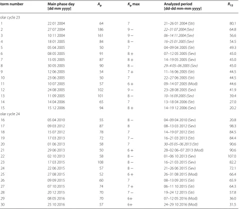
As each bin can contain a different number, NK, of pairs of measurements, the distance pertinent to each bin is Table 3 Storm time periods analyzed in this study
The main phase day (MPD), Ap daily mean, and Kp max geomagnetic indices values as recorded during the MPD, analyzed periods, and the R12 solar activity index are shown for each considered moderate (Mod), strong (Str), and severe (Sev) geomagnetic storm. Periods characterized by significant substorms are highlighted in italics
Storm number Main phase day
[dd mm yyyy] Ap Kp max Analyzed period [dd-dd mm-mm yyyy] R12
Solar cycle 23
1 22 01 2004 64 7 21–26 01 2004 (Str) 80.1
2 27 07 2004 186 9 − 22–31 07 2004 (Sev) 64.8
3 10 11 2004 161 9 − 06–14 11 2004 (Sev) 56.6
4 18 01 2005 84 8 − 16–25 01 2005 (Sev) 54.5
5 05 04 2005 50 7 04–09 04 2005 (Str) 49.3
6 08 05 2005 91 8 + 07–12 05 2005 (Sev) 45.0
7 15 05 2005 87 8 + 14–19 05 2005 (Sev) 45.0
8 30 05 2005 90 8 − 29–4 05–06 2005 (Sev) 45.0
9 12 06 2005 54 7 + 11–16 06 2005 (Str) 44.5
10 23 06 2005 50 7 22–27 06 2005 (Str) 44.5
11 10 07 2005 57 6 + 09–14 07 2005 (Mod) 44.6
12 24 08 2005 102 9 − 23–28 08 2005 (Sev) 41.9
13 11 09 2005 101 8 − 10–16 09 2005 (Sev) 39.4
14 14 04 2006 65 7 13–18 04 2006 (Str) 27.0
15 15 12 2006 94 8 + 14–19 12 2006 (Sev) 20.2
Solar cycle 24
16 05 04 2010 55 8 − 04–09 04 2010 (Sev) 20.8
17 09 03 2012 87 8 08–13 03 2012 (Sev) 98.3
18 15 07 2012 78 7 14–19 07 2012 (Str) 84.5
19 17 03 2013 72 7 − 16–21 03 2013 (Str) 84.4
20 01 06 2013 58 7 30–05 05–06 2013 (Str) 90.6
21 29 06 2013 50 6 + 28–02 06–07 2013 (Mod) 90.6
22 02 10 2013 58 8 − 01–06 10 2013 (Sev) 107.0
23 17 03 2015 108 8 − 16–21 03 2015 (Sev) 82.2
24 22 06 2015 57 8 − 21–26 06 2015 (Sev) 72.1
25 27 08 2015 52 6 + 26–31 08 2015 (Mod) 66.4
26 09 09 2015 60 7 08–13 09 2015 (Str) 65.9
27 07 10 2015 74 7 + 06–11 10 2015 (Str) 64.3
28 20 12 2015 70 7 − 19–24 12 2015 (Str) 57.8
29 08 05 2016 70 6+ 07–12 05 2016 (Mod) 36.0
then defined as the average value, h¯
K , of the distances hk “falling” inside the bin
As a consequence, the semivariance associated with a given bin is the average value of the semivariances γ(hk) “falling” inside that bin
the plot obtained with the K points (one for each bin) of coordinates ( h¯
K , γ¯K ) constitutes the experimental variogram.
It is hence possible to “build” an experimental vari-ogram based on the assimilated measurements recorded in the reference stations. It depends essentially on how the reference stations are distributed over the consid-ered area. Data assimilation from many reference sta-tions located close to each other is important to catch the small-scale spatial structures, because it populates the
(7) ¯
hK = NK
k=1hk NK
.
(8) ¯
γK =
NK
k=1γ (hk) NK
= 1 2(NK)
NK
k=1
z(xk)−z(x′
k)
2 ;
part of the variogram near the origin. The assimilation of data from reference stations placed far from each other is instead fundamental for the description of the large-scale spatial behavior.
Once the variogram is “built,” there is the need to find a mathematical function which fits the experimental data. The mathematical expressions that can be used to fit the experimental variogram correspond to five commonly used variogram models: linear and power (non-stationary models), gaussian, spherical, and exponential (stationary models).
The distinction between stationary and non-stationary models depends on their behavior at distances compa-rable to the size of the domain. When the experimental variogram presents a steady trend around a value, called
sill (σ2), as the distance increases, it is possible to define a length scale, called range (α), at which the sill is obtained.
mathematical functions describing the various variogram
exhibiting a parabolic behavior around the origin; 4. Spherical:
exhibiting a linear behavior around the origin; 5. Exponential:
exhibiting a linear behavior around the origin.
It is important to keep in mind that each variogram model embeds, with a different degree of reliability, the information concerning the small- and large-scale behav-ior of the parameter under study. That is why the selec-tion of the variogram model plays a fundamental role in determining the quality and reliability of the prediction map over the area under consideration.
The observation at the point of coordinate x0 can be represented as
where m(x0) is the deterministic part of z(x0) represent-ing the large-scale spatial variability, while ε(x0) is the stochastic part of z(x0) which describes, particularly for stationary variogram models, the small-scale spatial vari-ability. In the Ordinary Kriging method, m(x0) = m, i.e., it is a constant which does not depends on the spatial coordinates. Since the electron density presents values at mid-low latitudes higher than the ones at mid-high latitudes, there exists a latitudinal spatial gradient char-acterizing the ionospheric characteristics which we are
(9)
going to describe. This fact makes the Universal Krig-ing method (UKM) particularly suitable to describe the variability of the ionospheric characteristics under study, because UKM takes into account also the spatial gradi-ents by means of additional terms, so that the term m(x0), also called drift part, is written as
where f1(x0),…., fp(x0) are functions of spatial coordinates generally known, and β1,…, βp are the so called drift coef-ficients, which are usually unknown.
In our specific case the term m(x0) is written as:
being φ0 and λ0 the longitude and latitude of the point x0, which are known, while the coefficients A, B, and C must be determined. The combination of Eq. (15) with Eq. (16) gives f1(xi) = 1, f2(xi) = φ0, and f3(xi) = λ0.
Combining Eq. (14) with Eq. (15), we get
With regard to the issue dealing with the stochastic part
ε(x0), being the topic out of the context of this work, we invite the interested reader to refer to Section 3.3 of Pig-nalberi et al. (2018a) and to Kitanidis (1997).
On the choice of the best variogram model in the Universal Kriging procedure: a new quality check routine (NQCR)
As already explained by Pignalberi et al. (2018a, b), reli-able foF2, M(3000)F2, and hmF2 maps can be obtained when the IRI model is updated with a realistic IG12eff and R12eff representation. Such representation is obtained applying the UKM on a discrete set of IG12eff and R12eff values, obtained at the locations of selected reference sta-tions. It must be pointed out that the UKM provides a variogram model which, in principle, should be the one that best fits the experimental variogram (i.e., the vari-ogram built on the discrete set of IG12eff and R12eff values). Therefore, the problem of how to choose among the possible variogram models described in “The Kriging interpolation method: a brief recall” section is of cru-cial importance, because this choice greatly affects the goodness of the IG12eff and R12eff maps and, consequently, the capability of delivering an accurate and trustworthy
the preliminary quality check of the variogram model, based on the evaluation of the exponent s (0 < s < 2) of the power variogram model, was developed in the IRI UP method.
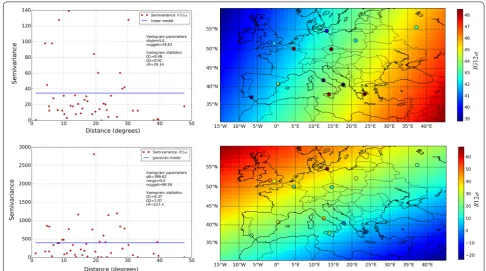
In cases for which s is close to 0, the variogram model is an approximately straight horizontal line, while in cases for which s tends to 2 the variogram model has an approximately parabolic behavior at both small and large scales (Kitanidis 1997). For s ≪ 1 the semivariance does not vary with the distance, as it should be expected; therefore, these cases correspond to unrealistic situations which would lead to unrealistic maps of IG12eff and R12eff. For this reason, for the preliminary quality check of the variogram model, we have set a very low threshold value for s (sthrs = 0.1) discarding those variograms for which s < sthrs. Examples of variogram models and related maps of IG12eff and R12eff discarded by the IRI UP method are shown in Fig. 3. The meaning of the associated statistics parameters Q1, Q2, and cR written in the legend will be clarified in the next sections.
It should be noted that s < sthrs does not provide an objective criterion, because sthrs is the same for each vari-ogram model. That is why in this work the IRI UP method has been updated by the NQCR procedure to choose the best variogram model, through appropriate statistical tests.
Q1 statistics
Residuals are the differences between observations and model predictions. In statistical modeling (regression, time series, analysis of variance, and geostatistics), the param-eter estimation and the model validation depend heavily on the examination of residuals.
We can define the variable
where n is the number of observations and εk = Sδk
k are the normalized residuals, being δk the common residuals and Sk the variance of their distribution. It can be proven (see Kitanidis 1997) that Q1 is a statistical variable which follows the normal distribution with a probability density function (PDF) given by
with a mean value m= 0 and a variance σ2= n−11. Therefore, we have a probability of about 95% that Q1 is ranged in the interval
(18) Q1=
1 n−1
n
k=2
εk,
(19)
f(Q1)= 1
2π
n−1 e
−
Q21
2
n−1
,
and a probability of about 68% that Q1 is ranged in the interval
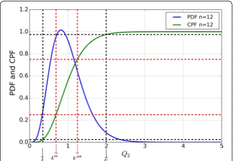
An example of the PDF and the cumulative probability function (CPF) of the variable Q1, obtained for n = 12, is shown in Fig. 4.
When the condition (20) is fulfilled, the variogram model under examination is accepted and it is signifi-cant from the statistical point of view with a probability of about 95%; this implies that there exists a 5% of prob-ability to accept an incorrect variogram model. However, a 5% cutoff is customary in statistics. Therefore, when (20) is met, we can assume that the variogram model has passed the Q1 statistical test.
Q2 statistics
Another test that can be carried out to test the goodness of the variogram model is that relying on the statistical variable Q2 defined as
(20) −2σ <Q1<+2σ i.e. |Q1|<
2 √
n−1,
(21) −σ <Q1<+σ i.e. |Q1|<
1
√
n−1.
(22) Q2=
1
n−1
n
k=2 ε2k.
It can be proven (see Kitanidis 1997) that Q2 is a statisti-cal variable whose PDF is
with a mean value m → 1, for n → ∞ , and a variance σ2= n−21.
An example of the PDF and CPF of the variable Q2, obtained for n = 12, is shown in Fig. 5.
Therefore, according to Fig. 5, if the value of Q2 given by Eq. (22) is included in the interval
the variogram model under examination is significant from the statistical point of view with a probability of 95%. When this condition is met, we could say that the variogram model has passed the Q2 statistical test to the usual confidence level of 5%, in the sense that there exists, however, a 5% probability that an incorrect vari-ogram model is accepted.
It is worth noting that the form of PDF and CPF depends on the number n of assimilated ionosonde data and, consequently, the same stands for the values of the two thresholds (L, U) and (L1st, U3rd).
(23)
f(Q2)=
(n−1)n−21Q
n−3 2 2 e
− (n−1)Q
2 2
2n−21Γ
n−1
2
,
(24)
L<Q2<U,
Fig. 4 Probability density function and cumulative probability function for the Q1 variable. Example of PDF (solid blue line)
and CPF (solid green line) for Q1, for n = 12. Red and black
arrows (corresponding to red and black dashed vertical lines) indicate, respectively, the thresholds ± 1σ and ± 2σ. Black and red dashed horizontal lines represent the values referred to the CPF corresponding to the conditions (20) and (21) which, for the considered case, provide, respectively, the numerical solutions
− 0.60 < Q1 < + 0.60 and − 0.30 < Q1 < + 0.30
Fig. 5 Probability density function and cumulative probability function for the Q2 variable. Example of PDF and CPF for Q2 for n = 12. The black dashed horizontal lines intersect the CPF at the two points of coordinates (L, 0.025) and (U, 0.975), while the red dashed horizontal lines intersect the CPF at the two points of coordinates (L1st, 0.25) and (U3rd, 0.75), where L1st and U3rd identify the
The cR criterion
The residuals are particularly important in evaluat-ing how closely the variogram model fits the data, since smaller residuals imply a better fit. To construct stable (i.e., less affected by random error) criteria for the choice of the best variogram model, we may also use the stabi-lized geometric mean of the residuals’ variance (Sk), sub-ject to the constraint Q2 = 1 (see Kitanidis 1997), i.e., the parameter
The condition
allows to choose among the various variogram models.
Q1, Q2, and cR statistical test: some results
The statistical criteria (20), (24), and (26) described in the previous sections constitute the NQCR procedure imple-mented in the IRI UP method.
For the selection of the “best” variogram model, one could be tempted to consider only the cR criterion, leav-ing out the criteria (20) and (24). Nevertheless, from a preliminary investigation conducted over a large number of variogram models, we realized that if only the cR crite-rion were applied, several variogram models which do not satisfy the criteria (20) and/or (24) would be accepted.
(25)
cR=e
1
n−1 n
k=2ln(Sk2)
.
(26)
cR= minimum,
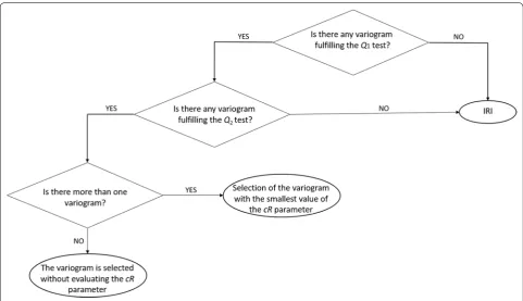
For these reasons, we decided to proceed to the selec-tion of the variogram through an iterative procedure that NQCR applies following the flowchart depicted in Fig. 6. The figure shows just an example of how the NQCR procedure can be applied on each of the epochs (dd/ mm/yyyy/hh) listed in Table 3 and illustrates, in general terms, the various steps carried out in order to select that variogram model which, to an acceptable degree of confi-dence, fits the data more reliably than the other ones.
Figure 7 shows some examples of spherical and linear variogram models which have met the requirements (20), (24), and (26) and that therefore have been selected to get a statistically significant IG12eff, and R12eff modeling and, consequently, a reliable mapping of foF2 and M(3000)F2 and, hence, of hmF2. Note that the variograms reported in Fig. 7, matching the requirements (20), (24), and (26), automatically fulfill also the previous quality check
s < sthrs.
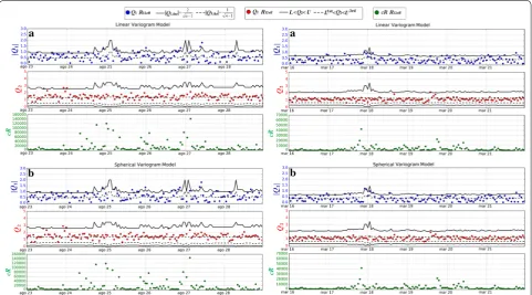
Some examples of Q1, Q2, and cR time series, for linear and spherical variogram models used to obtain
IG12eff and R12eff maps, are shown in Figs. 8 and 9, respectively. For the Q1 statistical test, each case exceeding the threshold (20) is rejected, as well as for the Q2 statistical test each case not included in the interval (24) is refused. Note that the epochs character-ized by the greatest values of cR are those following the main phase of the storm.
Blue, red and green dots represent the values of Q1, Q2, and cR, respectively, computed by Eqs. (18), (22), and (25). We want to stress once again here the fact that for the Q1 and Q2 statistics the thresholds depend on the number n of foF2 and M(3000)F2 values available in the reference stations which, at a given hour, have been con-sidered according to the criteria described in “ Descrip-tion of the filter implemented to select ionosonde data” section. Obviously, the value of n can be different from epoch to epoch because, at a given moment, it is possi-ble that a station is not working and/or the ionospheric characteristics of a station are wrongly autoscaled.
This explains why the continuous black lines represent-ing the Q1 and Q2 thresholds in Figs. 8 and 9 are not flat. The implementation of the NQCR procedure constitutes then an important difference with respect to the pre-liminary quality check based only on the exponent s for which, whatever is the epoch and variogram model under study, the threshold value sthrs is not a function of n but it is fixed to 0.1.
Validation of IRI UP method including the F algorithm and the NQCR procedure: some results The IRI UP method, embedding the F algorithm and the NQCR procedure, as described, respectively, in “ Descrip-tion of the filter implemented to select ionosonde data”
and “On the choice of the best variogram model in the Universal Kriging procedure: a new quality check routine (NQCR)” sections, has been systematically tested over the 30 disturbed time intervals listed in Table 3, in order to investigate its performance during moderate, strong, and severe geomagnetic storms.
For each epoch, the testing procedure follows four steps:
1. the variogram models which have passed the Q1 and
Q2 statistical tests (as, for example, those fitting the
IG12eff and R12eff experimental variograms of Fig. 7) and the cR criterion are considered;
2. applying the UKM for each selected variogram model, IG12eff and R12eff maps are calculated over the European area depicted in Fig. 1;
3. foF2 and M(3000)F2 maps are calculated giving as input to the IRI model the IG12eff and R12eff maps cal-culated in 2); then, applying the empirical formula which relates hmF2 to foF2 and M(3000)F2 (Bilitza et al. 1979), also hmF2 maps are obtained;
4. from foF2 and hmF2 maps, values at the truth sites of Fairford and San Vito are extracted and compared with corresponding measurements.
Fig. 8 Q1, Q2, and cR time series for IG12eff, for selected storms and variogram models. Q1, Q2, and cR time series for a linear and b spherical variogram models for IG12eff corresponding to the severe geomagnetic storms listed in Table 3 as number 12 (left) and 27 (right). The continuous and dashed black lines in Q1 and Q2 plots represent the threshold values as highlighted at the top of the figure
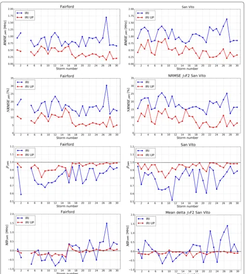
For each storm the following statistical parameters are calculated:
where N is the number of epochs that constitute the con-sidered storm, X stands for foF2 or hmF2, the subscript modeled stands for IRI UP or IRI predicted values (the IRI model is considered with the storm option “ON”), while the subscript ionosonde refers to values recorded by the ionosonde;
where X¯ionosonde is the arithmetic mean over time of X ion-osonde values;
where cov() is the covariance, while σXmodeled and σXionosonde are the standard deviations;
In addition, also the percentage of discarded maps is calculated:
where goodmaps is the number of IG12eff or R12eff maps passing the first two steps of the NQCR procedure, i.e.,
Q1, and Q2 tests, and totalmaps is the total potential number of maps.
Figures 10 and 11 show some examples of compari-son between IRI and IRI UP, in terms of the aforemen-tioned statistical quantities carried out at Fairford and San Vito for each storm listed in Table 3, for both foF2 and hmF2.
Figure 12 shows, for each storm individually and for the whole group of storms, the percentage of discarded vari-ogram models calculated by Eq. (31).
Finally, the MDX quantities provided by Eq. (30), taken as absolute values (to avoid that positive and negative val-ues around zero could cancel each other), have been used to calculate the following mean value:
(27)
Root Mean Square Error, RMSEX
= Normalized Root Mean Square Error,
NRMSEX =
RMSEX ¯
Xionosonde,
(29)
Pearson Correlation Coefficient, ρX
= cov(
Xmodeled,Xionosonde)
σXmodeledσXionosonde ,
%discarded= totalmaps−goodmaps totalmaps ,
Tables 4 and 5 summarize the statistical results calculated by Eqs. (27)–(29) and Eq. (32) at the truth sites of Fair-ford and San Vito for foF2 and hmF2, respectively, in the following three cases: (a) IRI UP method running with a fixed variogram model (like in Pignalberi et al. 2018a) and considering only those cases passing the first two steps of the NQCR procedure, namely Q1 and Q2 tests; (b) IRI background model; (c) IRI UP method embedding the complete NQCR procedure.
The winning percentage of each variogram model is computed for each single storm and for the complete storm set, evaluating the following parameters
where i is the index running on the 5 possible variogram models, ss is the index running on the considered storms,
nss,i is the number of times the i variogram model is declared as the “winner” by the NQCR for the storm ss, and Nss is the total number of epochs included in each single storm ss.
Figures 13a and 14a show the winning percentage of each variogram model for each single storm, for IG12eff and R12eff, respectively; Figs. 13b and 14b show the same percentage for the complete storm set.
Discussion, conclusions, and future developments In this investigation the IRI UP method was upgraded by applying the F algorithm and the NQCR procedure to select the best variogram model.
The F algorithm described by Eqs. (1)–(4) has proven to be very effective in disregarding ionosonde data which, once assimilated, would affect badly the mod-eling of IG12eff and R12eff, leading to unrealistic foF2 and M(3000)F2 maps and, consequently, to unlikely hmF2 maps (Pignalberi et al. 2018a, b). It must be noted that considering five standard deviations and thresholds values for the standard deviation equal to 0.5 MHz, for
foF2, and 0.15, for M(3000)F2, are subjective choices, aiming to remove especially those measurements which are clearly out of range (spikes), as shown in Fig. 2.
Using residuals it is possible to define the statistical parameters Q1 and Q2 along with their PDF and CPF, which are sketched in Figs. 4 and 5, respectively, for a number of reference stations equal to 12. In these figures,
the two thresholds |σ| and |2σ| for Q1, and [L–U] and [L1st–U3rd] for Q
the number of discarded variogram models. In fact, in Figs. 8 and 9, for the storm number 12 (August 23–28, 2005), it clearly emerges that the number of rejected vari-ogram models is relatively large when the threshold is lowered from |2σ| to |σ| (for the statistical test Q1) and
from [L–U] to [L1st–U3rd] (for the statistical test Q 2). The threshold effect is however much less evident in the case of the storm number 27 (October 6–11, 2015), for which a limited number of variograms are discarded when reducing the threshold.
This is probably due to the different numbers of avail-able reference stations used in the assimilation, which for the period October 6–11, 2015 (n = 12), is larger than that for the period August 23–28, 2005 (n = 8), thus
allowing a better representation of the spatial gradients over the area under study.
When the distribution of semivariance values cal-culated through Eq. (6) is such that the experimental Fig. 12 Percentage of variogram models discarded by the NQCR procedure. Percentage of discarded variogram models for (top) each storm listed in Table 3 and (bottom) all storms as a whole, for (left) foF2 and (right) hmF2. On the top panels the percentage of the linear model is not visible because hidden by the power model
Table 4 Statistical validation of foF2 as modeled by IRI UP and IRI
Statistical results for foF2 obtained at the two truth sites of Fairford and San Vito for: IRI, IRI UP running with a fixed variogram model (IRI UP—variogram model chosen in the table), and IRI UP embedding the NQCR procedure (italics)
Station Ionospheric
characteristic Model RMSE (MHz) NRMSE (%) ρ MMDX AV [MHz]
Fairford foF2 IRI UP—linear 0.474 9.40 0.927 0.137
IRI UP—power 0.471 9.37 0.929 0.139
IRI UP—Gaussian 0.467 9.28 0.920 0.152
IRI UP—spherical 0.464 9.23 0.926 0.146
IRI UP—exponential 0.461 9.14 0.927 0.144
IRI 0.865 16.85 0.824 0.415
IRI UP 0.401 8.25 0.947 0.122
San Vito foF2 IRI UP—linear 0.558 9.74 0.927 0.088
IRI UP—power 0.555 9.69 0.927 0.090
IRI UP—Gaussian 0.538 9.38 0.922 0.083
IRI UP—spherical 0.539 9.39 0.927 0.088
IRI UP—exponential 0.538 9.36 0.927 0.090
IRI 1.075 18.37 0.797 0.374
Table 5 Statistical validation of hmF2 characteristic as modeled by IRI UP and IRI
Same as Table 4 but for hmF2
Station Ionospheric
characteristic Variogram model RMSE (km) NRMSE (%) ρ MMDXAV (km)
Fairford hmF2 IRI UP—linear 31.567 11.31 0.817 7.361
IRI UP—power 31.552 11.27 0.819 7.376
IRI UP—Gaussian 30.334 10.83 0.796 7.457
IRI UP—spherical 30.744 10.97 0.811 7.388
IRI UP—exponential 30.844 11.00 0.811 7.479
IRI 35.241 12.57 0.797 9.879
IRI UP 29.369 10.44 0.845 6.844
San Vito hmF2 IRI UP—linear 30.132 10.62 0.798 7.469
IRI UP—power 30.197 10.64 0.799 7.674
IRI UP—Gaussian 28.193 10.19 0.780 8.162
IRI UP—spherical 29.805 10.50 0.783 8.053
IRI UP—exponential 29.685 10.46 0.792 7.901
IRI 33.252 11.70 0.749 9.577
IRI UP 24.671 8.62 0.859 6.959
Fig. 13 Percentage of IG12eff variogram models declared winners by the NQCR procedure. a Winning percentages related to each IG12eff variogram
model, for each single storm, after applying the NQCR procedure sketched in Fig. 6; b same as a but considering all storms listed in Table 3 as a whole
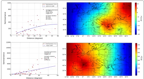
variogram cannot be adequately represented by any of the variogram models defined in “The Kriging interpolation method: a brief recall” section, we are forced to discard the variogram modeling because it would lead to unre-alistic maps. Figure 3 shows some examples of discarded variogram models for IG12eff and R12eff; in these two cases the fitting function is an approximately straight horizon-tal line whatever is the considered variogram model, and the corresponding maps are not able to reproduce IG12eff and R12eff values over the reference stations. This is due to the very large nugget values (c0 = 34.8 for IG12eff and c0 = 98.6 for R12eff) describing the microscale variability. This implies that colored dots, marking the reference sta-tions, are in contrast with the colors characterizing the regions around the reference stations, which means that the maps are not realistic since do not match the meas-ured data.
On the other hand, if in Fig. 3 we look at the statisti-cal parameters related to these two experimental vari-ograms, the associated values of Q1 (0.49 for IG12eff, 0.37 for R12eff) and Q2 (0.91 for IG12eff, 1.07 for R12eff) are such that the two experimental variograms do not pass the Q1 and Q2 statistical test defined in “Q1 statistics” and “Q2 statistics” sections, and hence, they must be rejected along with their corresponding maps.
On the contrary, when the nugget effect is not so rel-evant and the distribution of semivariance values can be well described by most variogram models, the experi-mental variograms produce realistic maps. This is what happens for the case shown in Fig. 7 where the null nug-get effect (c0 = 0 for IG12eff and R12eff), and the associated values of Q1 (0.22 for IG12eff, 0.49 for R12eff) and Q2 (0.98 for IG12eff, 0.76 for R12eff) are such that the two experi-mental variograms pass both the Q1 and the Q2 statisti-cal test. In this case, the corresponding maps show IG12eff and R12eff values, over the reference stations, compatible with those of the regions close to the reference stations.
The preliminary quality check based on the exponent s
sets always the same threshold value sthrs = 0.1 whatever is the epoch and variogram model under study, without taking into account that the goodness of the variogram model depends also on the number n of available iono-sonde data which are going to be considered in the UKM. This significant limitation characterizing the first ver-sion of IRI UP is overcome because, through the NQCR procedure, the quality check now depends on the n value that can change from epoch to epoch. Moreover, another essential aspect that should be considered when NQCR is applied is that, from a scientific point of view, “win-ning” variogram models are more reliable than the ones which have passed only the s ≥ sthrs test. As it is easy to realize looking at Figs. 8 and 9, the number of variogram models discarded by the NQCR procedure depends on
the established thresholds values. As a general rule, if, at a given epoch, the number of reliable ionosonde data to be assimilated is relatively large, we can choose a more selective threshold, thus providing ionospheric character-istics maps with a high confidence level. In the event that the number of reliable ionosonde data is lower, we have to increase the threshold and in this case a map can be provided, but at a lower confidence level. It is clear that when there are very few reliable data to be assimilated, we cannot provide a statistically significant updated map. In this case the IRI UP method is not applicable and we rely on the IRI background map.
IRI UP and IRI prediction maps of the ionospheric characteristics foF2 and M(3000)F2, relative to 30 geo-magnetic storms occurred between January 1, 2004, and December 31, 2016, are used to generate IRI UP and IRI prediction maps of hmF2 using Bilitza et al. (1979). The values of foF2 and hmF2 extracted at the two truth sites of Fairford and San Vito from the corresponding IRI UP and IRI prediction maps have been compared with the measurements, to compare IRI UP and IRI performance.
The obtained results confirm those shown in Pignalberi et al. (2018a, b) for the St. Patrick geomagnetic storm; in fact, as shown in Figs. 10 and 11, as well as in Tables 4
and 5, they indicate that IRI UP performs significantly better than IRI, for all the 30 considered cases.
Moreover, results of Tables 4 and 5 show that when IRI UP is applied deciding a priori the variogram model, and then considering only those cases passing the first two steps of the NQCR procedure, a clear difference among the various variogram models does not emerge.
In fact, NRMSE values for foF2 and hmF2 range, respectively, between 9.14 and 9.40% and between 10.83 and 11.31% at Fairford and between 9.36 and 9.74% and between 10.19 and 10.64% at San Vito, while MMDX AV values for foF2 and hmF2 range, respectively, between 0.137 and 0.152 MHz and between 7.361 and 7.479 km at Fairford and between 0.083 and 0.090 MHz and between 7.469 and 8.162 km at San Vito.
When the IRI UP method runs with the complete NQCR procedure, its performance shows a noticeable improvement at the considered truth sites, for both foF2 and hmF2. In fact, in this case, NRMSE values for foF2 and hmF2 are 8.25% and 10.44% at Fairford and 8.70% and 8.62% at San Vito, while MMDX AV values for foF2 and hmF2 are 0.122 MHz and 6.844 km at Fairford and 0.084 MHz and 6.959 km at San Vito.
the IRI UP method is effective in providing more precise and accurate results.
In general, from Figs. 10 and 11 it emerges that IRI UP performs slightly better for foF2 than for hmF2. This hap-pens for different reasons:
1. foF2 assimilated data are generally more reliable than the corresponding M(3000)F2 data. This is mostly due to the fact that ionograms can be characterized by multiple reflections of the F2 layer, and when this happens an autoscaling program can be misled and the second-order reflection can be identified as the real trace; in this case the foF2 value is usually not affected by a significant error, while the M(3000)F2 is significantly wrongly scaled (Scotto and Pezzopane
2008);
2. the spherical harmonic expansion used by IRI to describe the foF2 and M(3000)F2 spatial behavior (see Eq. (1) in Pignalberi et al. 2018a) stops when the maximum order of the harmonics is equal to 76, for
foF2, and to 49, for M(3000)F2, which means that
foF2 maps present a higher spatial resolution than
M(3000)F2 ones;
3. hmF2 is calculated applying the empirical formula of Bilitza et al. (1979), and this implies that the error characterizing hmF2 depends on the errors relative to
foF2, M(3000)F2, foE (the E-layer critical frequency), and R12eff.; therefore, the error propagation leads to an error associated with hmF2 which is intrinsically larger than that of foF2;
4. last but not least, foF2 predictions are based on the
IG12eff index, which is an ionospheric index because it is “built” just starting from foF2 values recorded at several ionospheric stations (Liu et al. 1983), while
M(3000)F2 predictions, which come into play to cal-culate hmF2, are not based on an ionospheric index, but on R12eff.
Another positive aspect of the IRI UP method is that the experimental variogram has a higher spatial variability the larger is the number n of data assimilated from the reference stations, so that corresponding maps are statis-tically more reliable and are not discarded. This situation is clear from the results of Fig. 12 where, for each kind of variogram model, a decreasing trend of the number of discarded maps is observed starting from the storm num-ber 17, corresponding to 2012, i.e., the year from which the number of available ionospheric stations maximizes (see Table 2).
It is also to be noted that stationary variogram models (gaussian, spherical, and exponential) are more sensi-tive than non-stationary ones to the number n of assimi-lated data; this is probably due to their more complex
mathematical formulation which requires a greater value of n to represent more adequately the spatial correlations between measurements, for every spatial scale. In fact, considering all storms as a whole, it results that percent-ages of rejected stationary variograms for foF2 (Fig. 12c) and hmF2 (Fig. 12d) are greater than those related to non-stationary variograms (linear and power). This result is probably due to the cumulative effect of the first 16 storms listed in Table 3, which are relative to years characterized by a low value of n. Nevertheless, in Fig. 12a, b, the trend observed starting from the storm number 17, correspond-ing to the years for which n is increased (n = 12), suggests that the percentages of stationary and non-stationary dis-carded variogram models may converge to similar values as the number of stations increases.
The winning percentages shown in Figs. 13b and 14b indicate that among the linear, power, spherical, and exponential variogram models there is not a clear pre-dominance of one model over another, and that the gaussian variogram model shows the higher percent-ages, ≈ 40% and 29%, for IG12eff and R12eff, respectively. This fact is surprising, because if we consider Fig. 12 the Gaussian model is the one most rejected. This means that the Gaussian variogram model passes more difficult the
Q1 and Q2 statistical tests, but when this happens, it is more likely to be the best according to the NQCR pro-cedure. A fact that clearly emerges also when each single storm is considered (Figs. 13a, 14a).
It is worth noting that the achieved results have been obtained without explicitly considering the hour of the day. In fact, with regard to the future developments, a very important aspect that will have to be considered is that ionospheric characteristics depend inherently on the hour of the day. At the solar terminator (hours around sunrise and sunset), regardless of the large-scale latitu-dinal spatial gradients, the electron density spatial dis-tribution manifests also large longitudinal gradients on small spatial scales. On the contrary, under ionospheric stationary conditions (hours around noon and midnight) the electron density spatial distribution does not show large longitudinal differences and hence the ionospheric variability is characterized by small gradients on both large and small spatial scale. These considerations imply that the choice of the variogram model should depend on the hour of the day.
This means that stationary variogram models (Gaussian, spherical, and exponential) could describe better the situa-tions at the sunrise and sunset hours, when the ionospheric characteristic shows large gradients on small spatial scale.
Vice versa, in the hours around noon, when the small-scale spatial gradients are not so important, non-station-ary variogram models (linear and power) are likely more indicated.
In the light of these considerations, a careful and detailed study, aimed to investigate how the hour of the day affects the choice of the variogram model, is of cru-cial importance to get useful clues in order to improve further the goodness of the variogram model selection and consequently the quality of prediction maps of the main ionospheric characteristics.
The results achieved in this investigation prove, how-ever, that reliable and trustworthy updated maps of the main ionospheric characteristics can be provided with a satisfactory degree of confidence, especially under moderate, strong and severe geomagnetic storm condi-tions. This means that IRI UP method, embedding the F algorithm and the NQCR procedure, represents an interesting approach to Space Weather forecast in the ionospheric domain, for any region characterized by an adequately distributed network of ionosondes.
Abbreviations
ARTIST: Automatic Real-Time Ionogram Scaler with True height; CPF: cumula-tive probability function; CS: Confidence Score; HF: high frequency; IRI: International Reference Ionosphere; IRI UP: International Reference Ionosphere UPdate; ISP: IRI-SIRMUP-P; KIM: Kriging interpolation method; MD: Mean Delta; MMDAV: Mean Mean Delta absolute value; MPD: main phase day; NQCR: new quality check routine; NRMSE: normalized root mean square error; PDF: probability density function; RMSE: root mean square error; SIRMUP: Simplified Ionospheric Regional Model UPdating; UKM: Universal Kriging method; UT: universal time; UV: ultraviolet.
Authors’ contributions
AP conceived the study, developed the IRI UP method improvements described in the paper, and made the statistical analysis needed to validate the new version of the method. MPi drafted the manuscript, gave important insights about the developed statistical procedures, and actively participated to the discussion of the results. MPe participated in the discussion of the sta-tistical results and helped to draft the manuscript. RR gave insights about the statistical analysis, participated in the discussion of the statistical results, and revised the manuscript. All authors read and approved the final manuscript.
Author details
1 Dipartimento di Fisica e Astronomia, Università di Bologna “Alma Mater Studiorum”, Bologna, Italy. 2 Istituto Nazionale di Geofisica e Vulcanologia, 00143 Rome, Italy.
Acknowledgements
This publication uses data from 14 ionospheric observatories in Europe, made available via the public access portal of the Digital Ionogram Database of the Global Ionosphere Radio Observatory in Lowell, MA. The authors are indebted to observatory directors and ionosonde operators for heavy investments of their time, effort, expertise, and funds needed to acquire and provide measurement data to academic research. The IRI team is acknowledged for developing and maintaining the IRI model and for giving access to the cor-responding Fortran code via the IRI Web site (http://irimo del.org/).
Competing interests
The authors declare that they have no competing interests.
Availability of data and materials
Ionosonde data used in this study are publicly available at the Digital Iono-gram Database (http://ulcar .uml.edu/DIDBa se/) and can be freely downloaded by means of the SAO Explorer software developed by the University of Mas-sachusetts, Lowell (http://ulcar .uml.edu/SAO-X/SAO-X.html). Geomagnetic indices were downloaded from the OMNIWeb Data Explorer—NASA site at
https ://omniw eb.gsfc.nasa.gov/form/dx1.html. The IRI model Fortran code is available via the IRI Web site (http://irimo del.org/). The datasets generated and/or analyzed during the current study are available from the correspond-ing author on reasonable request.
Funding
This work is funded by the Department of Physics and Astronomy of the University of Bologna via a doctoral scholarship for the Geophysics Doctorate School. The Istituto Nazionale di Geofisica e Vulcanologia (INGV) in Rome made available human and technological resources, and working space, needed to carry out this work.
Publisher’s Note
Springer Nature remains neutral with regard to jurisdictional claims in pub-lished maps and institutional affiliations.
Received: 1 August 2018 Accepted: 8 November 2018
References
Angling MJ, Khattatov B (2006) Comparative study of two assimila-tive models of the ionosphere. Radio Sci 41:RS5S20. https ://doi. org/10.1029/2005R S0033 72
Bibl K, Reinisch BW (1978) The universal digital ionosonde. Radio Sci 13:519–530. https ://doi.org/10.1029/RS013 i003p 00519
Bilitza D, Reinisch BW (2008) International reference ionosphere 2007: improvements and new parameters. Adv Space Res 42(4):599–609.
https ://doi.org/10.1016/j.asr.2007.07.048
Bilitza D, Sheikh M, Eyfrig R (1979) A global model for the height of the F2-peak using M3000 values from the CCIR numerical map. Telecommun J 46:549–553
Bilitza D, McKinnell LA, Reinisch B, Fuller-Rowell T (2011) The International Reference Ionosphere today and in the future. J Geod 85:909–920. https ://doi.org/10.1007/s0019 0-010-0427-x
Bilitza D, Altadill D, Zhang Y, Mertens C, Truhlik V, Richards P, McKinnell LA, Reinisch B (2014) The International Reference Ionosphere 2012—a model of international collaboration. J Space Weather Space Clim 4:A07. https :// doi.org/10.1051/swsc/20140 04
Bilitza D, Altadill D, Truhlik V, Shubin V, Galkin I, Reinisch B, Huang X (2017) International Reference Ionosphere 2016: from ionospheric climate to real-time weather predictions. Space Weather 15:418–429. https ://doi. org/10.1002/2016S W0015 93
Buonsanto MJ (1999) Ionospheric storms—a review. Space Sci Rev 88:563–601 Decker DT, McNamara LF (2007) Validation of ionospheric weather predicted
by global assimilation of ionospheric measurements (GAIM) models. Radio Sci 42:RS4017. https ://doi.org/10.1029/2007R S0036 32
Galkin IA, Reinisch BW (2008) The new ARTIST 5 for all digisondes. In: Iono-sonde Network Advisory Group Bulletin, in: IPS Radio and Space Services, Surry Hills, NSW, Australia, vol 69, pp 1–8. http://www.ips.gov.au/IPSHo sted/INAG/web-69/2008/artis t5-inag.pdf
Galkin IA, Reinisch BW, Huang X, Bilitza D (2012) Assimilation of GIRO data into a real-time IRI. Radio Sci 47:7. https ://doi.org/10.1029/2011R S0049 52
Houminer Z, Bennett JA, Dyson PL (1993) Real-time ionospheric model updat-ing. J Electr Electr Eng Aust 13(2):99–104