Hierarchical CoSaMP for compressively sampled sparse signals with nested structure

R E S E A R C H

Open Access

Hierarchical CoSaMP for compressively

sampled sparse signals with nested structure

Stefania Colonnese

, Stefano Rinauro, Katia Mangone, Mauro Biagi, Roberto Cusani and Gaetano Scarano

Abstract

This paper presents a novel procedure, named Hierarchical Compressive Sampling Matching Pursuit (CoSaMP), for reconstruction of compressively sampled sparse signals whose coefficients are organized according to a nested structure. The Hierarchical CoSaMP is inspired by the CoSaMP algorithm, and it is based on a suitable hierarchical extension of the support over which the compressively sampled signal is reconstructed. We analytically demonstrate the convergence of the Hierarchical CoSaMP and show by numerical simulations that the Hierarchical CoSaMP outperforms state-of-the-art algorithms in terms of accuracy for a given number of measurements at a restrained computational complexity.

1 Introduction

The burgeoning field of compressive sampling (CS) addresses the recovery of signals which are sparse either in the original domain or in a different representation domain achieved by a suitable invertible transform. The CS theory establishes conditions for sparse signals recov-ering from measurements acquired without satisfying the Nyquist criterion, provided that suitable relations between the number of measurements and the signal spar-sity are satisfied. CS studies encompass different issues, ranging from measurement acquisition via random pro-jections to signal recovery algorithms; besides, CS recon-struction algorithms possibly leverage specific signals underlying structure. The reconstruction algorithm Com-pressive Sampling Matching Pursuit (CoSaMP) by Needell and Tropp [1] represents a starting point in the defini-tion of reconstrucdefini-tion procedures. The reason is manifold. Firstly, its solid analytical derivation is viable of differ-ent extensions accounting for peculiar signal structures [2]. Secondly, its iterative structure may be extended to encompass prior knowledge on the signal to be recon-structed [3]. Besides, the CoSaMP gracefully degrades with noise, since the reconstruction error is bounded by a value proportional to the energy of the noise vector, for a sufficiently large number of measurements.

*Correspondence: stefania.colonnese@uniroma1.it

Dipartimento di Ingegneria dell’Informazione, Elettronica e delle

Telecomunicazioni (DIET), Università di Roma “La Sapienza”, Via Eudossiana 18, Rome 00184, Italy

In principle, the minimal number of measurements for the CoSaMP algorithm to converge on sparse noise-free signal is the least required by CS theory [1]. Still, in [4], it is observed that procedures exploiting the sparse signal structure can converge with a number of measurements of the order of the signal sparsity [5], whereas numerical examples show that the CoSaMP may require a number of measurements about four times larger than the signal sparsity. Thereby, it is argued that in specific applications, the number of measurements may be in principle suffi-cient to recover the signal under concern, exactly or in an approximate form, while still not being enough for the CoSaMP to converge. This limits the accuracy and applicability of CoSaMP in a variety of resource-limited applications, such as CS in sensor networks [6].

Several studies have been so far proposed to overcome the gap between the minimum number of measurements as predicted by CS theory and those required by the CoSaMP to converge. A fundamental study by Baraniuk et al. [2] proposes to exploit knowledge about peculiar structures exhibited by the sparse signal. Specifically, the authors focus on the reconstruction of K-compressible signals, e.g. signals that are approximately reconstructed by K coefficients, and show that if the signal presents a suitable structure, the reconstruction procedure can exploit this knowledge to constrain the recovered signal subspace and improve the accuracy for a given number of measurements.

The analysis in [2] introduces the concept of nested approximation property of a signal sparsity model to derive theoretical bounds for CS reconstruction. Further,

a prioriconstraints on the structure of the compressible signal, e.g. the organization in blocks or in a tree structure, are then invoked to take advantage of the signal spar-sity model and reduce the solution space of the recovery algorithm.

Herein, in the light of the work in [2], we concern ourselves with signals whose coefficients are organized according to a nested structure. For such signals, we introduce a modified version of the CoSaMP algorithm, referred to as Hierarchical CoSaMP (HCoSaMP), that exploits the underlying assumption that the signal is hierarchically structured. Specifically, in HCoSaMP, the estimated support is progressively extended from a hier-archical layer to another throughout different estimation stages. Different from the analysis in [2], only the assump-tion on the nested signal structure is needed to formally state the convergence of the HCoSaMP. Thereby, the herein presented analysis imposes mild assumptions on the signals, and it applies in general cases where struc-tured sparsity cannot be claimed. Besides, we provide application examples on images obtained by oceano-graphic monitoring [6,7] and natural images [8], as well as on texture images [9]. For the former cases, we select the well-known discrete wavelet transform as a sparsifying transform, whereas for the latter, we resort to the graph-based transform, originally established for depth map encoding, as a sparsity-achieving representation within the reconstruction procedure. In both cases, we show that our procedure outperforms state-of-the-art reconstruc-tion algorithms and proves extending the feasibility of the reconstruction in the presence of a reduced number of measurements.

The structure of the paper is as follows. In Section 2, we recall the CS basics, while in Section 3, we discuss the CS of a sparse signal with nested structure. In Section 4, we describe the HCoSaMP and outline the demonstration of its convergence, and in Section 5, we report the numerical simulation results. Finally, Section 6 concludes the paper.

2 Compressive sampling basics

Let us consider an imagex[n1,n2], and let us denote by xtheN×1 vector built by collecting its samples in lexi-cographic order; besides, let us assume thatxisK-sparse. Letydenote theM×1 vector of CS measurements, given by

y= ˜x+n (1)

where ˜ is a suitable M×N random sensing matrix,

and n is the M×1 acquisition noise. For perfect

reconstruction of x given y, the sensing matrix ˜ is

supposed to satisfy the restricted isometry property (RIP) [10]:

(1−δK)x22≤ ˜x22≤(1+δK)x22. (2)

It can be proved that a matrix ˜ with i.i.d. random entries drawn from a Gaussian distribution with zero mean and variance 1/Msatisfies the RIP with high proba-bility [11,12] provided that

M≥MK =Cm

Klog(N/K)

δ2_K . (3)

Similar results have been derived for different classes of random sensing matrices. The relation (3) binds the signal sparsityK and the minimal number of measurementMK

for the matrix˜ to obey the RIP with a given RIP constant valueδK; conversely, for aK-sparse signal, the RIP

con-stant valueδK with which a selected matrix˜ satisfies the

RIP depends on the available number of measurements

M(see [13] for a detailed discussion), and being fixed the value of M, the value ofδkincreases withK.

Often, the signal is assumed to be sparse under a spar-sifying transformation identified by a transform basis matrix. Then,xis expressed asx= αwhere the vec-torαcollects the transform coefficients and it is defined on a set L of cardinality |L| = N. With these posi-tions, and because of the decomposition in (5), we can rewrite the acquisition process in (1) via a sensing matrix def= ˜ as follows:

y=α+n. (4)

In the following, we refer to aK-sparse signal such that only K out of itsN transform coefficients are non-zero valued; besides, we denote by the support of the K

non-zero coefficients ofα, satisfying ⊆ Land having cardinality|| =K<N.

3 CS of a sparse signal with nested structure

Let us consider a group ofL+1 subsetsLi,i = 0,. . .,L

of the overall setL, such thatL0⊂ L1⊂ . . .LL= L. We

also consider a partition of the supportof the non-zero terms ofαinto a finite number of sets_l,l =0,. . .,Lof

The above partition is found, for instance, in the L

decomposition levels of the wavelet transform of a natural image, where the setL0can be associated to the indexes of the scaling coefficients, and the setsLl,l=1,. . .,Lcan

of the non-zero scaling coefficients, and the sets_l,l =

1,. . .,L correspond to the incremental supports of the non-zero coefficients found in each of theL_l’s. Although the most familiar, the wavelet domain is not the sole one in which a hierarchical organization of the transform coef-ficients is observed. In Section 5, we show with the help of numerical examples that the graph-based transform (GBT) transform of texture images reveals a hierarchical structure, too.

The signalxsatisfies the nested approximation prop-erty (NAP) if the support of the best (in the least squares sense)K-term approximation inLi includes the support

of the bestK-term approximation inLi−1for allK ≥K, and fori=1,. . .L. This property, referred to as the NAP, is invoked in [2] on structured sparse signal models to derive a tight bound on the number of CS measurements required for signal reconstruction. The therein presented recovery algorithm exploits a priori knowledge on the structured nature of the signal. Herein, we drop further hypotheses on the signal structure, and we elaborate on the nestedness of the signal support.

Let us then consider a signalxrepresented by a spar-sifying transform , and let us assume that it satisfies the NAP in the transform domain. We rewrite the vec-torαasα = _lαl, whereαl denotes a vector whose

entries coincide with α for indexes in _l and are zero otherwise. Each subsetαl of the elements ofαhas

spar-sityKl, and the union of thei’s up to thel-th, namely

∪l

λ=0λ, of cardinality Kl =

l

λ=0Kλ, yields the best

K_l-term approximation of the signal itself.

The vectorxcan then be expressed as the sum of the contributions due to the different transform domain layers

x=

where l denotes the restriction of to the column

indices ofpertaining to different disjoint sets_l. Because of the decomposition in (5), we can rewrite the acquisition process in (4) as follows:

y=

l

αl+n. (6)

For simplicity sake, and without loss of generality, let us first refer to a nested decomposition encompassing only two layers, i.e. l = {0, 1}. Under this position, we can rewrite (6) as

y=α0+α1+n=α0+e0. (7)

The formulation in (7) gives a simple and yet interesting insight on the CS acquisition process. To elaborate, theM

measurements collected in (7) can be interpreted as either (i) the acquisition of theK-sparse vectorα with a mea-surement noisenof energyn2or (ii) the acquisition of theK0-sparse vectorα0 with a measurement noisee0of

energye02, suitably boundedabecause of the RIP of the

matrix.

4 Hierarchical CoSaMP

Here, we propose a modified version of the CoSaMP pro-cedure for reconstructing sparse signals exhibiting the above introduced nested structure. In short, we show that a signal endowed by such nested hierarchical struc-ture can be reconstructed by recursive application of the core stage of the CoSaMP algorithm on progressively expanded supports. Furthermore, we show that the result-ing procedure, which we refer to as Hierarchical CoSaMP (HCoSaMP), requires a lower number of measurements than the original CoSaMP to incrementally reconstruct the signal up to its bestK-term approximation.

Before turning to mathematics, we make two observa-tions. Firstly, the reformulation (7) of the relation in (6) hints to recover the coefficients ofα0 starting from the measurements y, instead of trying to recover the whole

signal α. The requirement on the number of

measure-ments for the CoSaMP convergence in reconstructing the

K0samples of α0 is indeed looser than that for recon-struction of theKsamples ofα. Specifically, the number

Mmust satisfy the RIP forδ_4K0 but not forδ_4K [1]. If the RIP forδ_4K0 is satisfied, the samplesα0can be recovered by the CoSaMP algorithm [2] and numerical bounds relat-ing the estimation error to the signal energy out of₀are provided.

Specifically, in [1], the accuracy achieved at conver-gence by the CoSaMP algorithm is characterized by the following mean square error bound:

α−α02≤15

From (8), we recognize that the performance of such CoSaMP-based stage degrades gracefully as the energy

out of 0 increases, just as it occurs when CoSaMP

recovers noisy signals or compressible signals.

Secondly, let us assume to have recovered, to a cer-tain degree of accuracy, the samples α0 starting from the measurements collected as in (7), so as to have the bestK0-term approximation of the sparse signalα. Then, this coarse estimate can be adopted as a better initial-ization of a CoSaMP procedure, in order to recover the remainingK1−K0coefficients providing the bestK1-term approximation of theαitself.

then (ii) recursively injecting the coefficients recovered on the support _l−1 as initialization for recovering the coefficientsαlon the supportl.

The recovery stages (i) and (ii) are respectively realized according to Algorithms 1 and 2, where we denote by† the pseudo-inverse of , i.e. ∗−1∗; by xN the

restriction ofxto itsNlargest-magnitude components; by x|T(A|T) the restriction ofx(A) to the elements (columns)

of indices in the setT; and by|T|the cardinality of the set T.

To sum up, the outline of the HCoSaMP is as follows:

(a) Recovery of the first decomposition layer. The outline of this partial estimation stage appears in Algorithm 1; this stage encompasses all the steps of the CoSaMP, plus an additional step (namely step 3 in Algorithm 1, which tailors the support estimated at each iteration to the predefined supportL0.

(b) Recovery of thel-th decomposition layer. The outline of the estimation stage providing the reconstruction

Algorithm 1 Hierarchical CoSaMP - recovery of first decomposition level

Initialization:

1. α(0)₀ =0

2. r=y(starting residual)

loop on j

1. Evaluate proxy

u=∗r

2. Compute the best2Ksupport set of the proxy

ω=supp(u2K)

3. Restrict such a support toL0 ω0=L0∩ω

4. Mergeω₀with previous support

T=ω0∪supp(α(j−0 1))

5. Least-squares estimation

b|T=†_|Ty b|Tc =0

6. Updateα₀(j)as the coefficients ofbinsideL0 α(j)₀ =bL0

7. Evaluate next residual

r=y−α₀(j)

Upon expiration of a maximum number of iterations J

1. Output reconstruction ofα0 ˆ

α0=α₀(J)

of the signal up to the support_lgiven its previous estimate up to the support_l−1appears in

Algorithm 2. We recognize that this stage still reproduces the steps encompassed by the CoSaMP from which it differs because it is initialized with the reconstructed version ofαl−1and it limits the

estimate to the support∪l_λ=0λ.

Algorithm 2 Hierarchical CoSaMP - recovery of thel -th decomposition level

Initialization:

1. Initialize with the reconstruction of(l−1)-th layer

α_l(0)= ˆα(l−1)

2. Starting residual

r=y−αˆ(l−1)

3. Initialize the support set

T =supp(αˆ(l−1))

loop on j

1. evaluate proxy

u=∗r

2. Compute the best2Ksupport set of the proxy

ω=supp(u2K)

3. RestrictωtoLl

ω_l =L_l∩ω

4. Mergeω_lwith previously evaluated supports

T =ω_l∪supp(α(_lj−1))

5. Least-squares estimation

b|T =†_|Ty b|Tc =0

6. Updateα_l(j)as the coefficients ofbinsideLl

α_l(j)=bLl

7. Evaluate next residual

r=y−α(_lj)

Upon expiration of maximum number of iterations J

1. Output reconstruction ofαup to thel-th decomposition level

ˆ αl=

l−1

In the following subsection, we formally prove the con-vergence of the HCoSaMP algorithm on NAP signals.

4.1 HCoSaMP convergence on a sparse signal with nested

structure

The convergence theorem is presented in two parts, respectively establishing the convergence in Algorithm 1 (Part I) and in Algorithm 2 (Part II).

Theorem 4.1( Part I: Convergence of Algorithm 1). Let us considerα₀ ∈ L₀withL0 = |L0|, and a set of M CS

noisy measurementsyobtained asy=α₀+e0according

to (7). Ifexhibits a RIP constantδ_L0 ≤0.1for the value of M at hand, then it can be proved that the mean square error on the estimateα₀(j) obtained at the j-th iteration of the HCoSaMP algorithm can be upper bounded as follows:

α0−α(0j)2≤4−jα02+15e02. (9)

Proof.(Proof of Theorem 4.1, Part I) To prove the con-vergence of Algorithm 1, we follow the guidelines in [1], by adapting them to the nested signal structure invoked by the Hierarchical CoSaMP algorithm. Specifically, we show that the reconstruction error at thej-th iteration of the algorithm

α₀−α(₀j)₂ (10)

is upper bounded by a term that, in the case of noise-free acquisition, decays asymptotically to zero. Towards this aim, we prove a series of inequalities providing the desired result.

At each iteration of the algorithm, the reconstructed sig-nalα₀(j) is selected as the restriction of the least squares estimatebover the supportL0. Based on such a restric-tion, considering that α0 lives, by definition, over the supportL0, we can write

α₀−α(₀j)₂= α₀−bL02≤ α0−b2. (11)

The following Lemma 4.1 provides an upper bound over the right-hand side of (11), representing the energy of the error of the least squares estimation in Algorithm 1.

Lemma 4.1. Let us consider the set T estimated as in Algorithm 1, and let b represent the LS estimate of the signal samples evaluated on the support T:

b|T =†_|Ty=

†

|T(α0+e0) b_|TC =0

. (12)

The energy of the estimation error is upper bounded by a term proportional to the energy of the signal α0over the

support TC and by a term proportional to the measure-ment noise energy:

α0−b2≤ α0|TC

1+ δL0 1−δ_L0 +

e0

1−δ_L0. (13)

The proof of Lemma 4.1 is found in Appendix 1. We recognize that the termα_0|TCin (13) represents

the energy of the original signalα_0|TC outside the setT.

Sinceα(₀j)has no energy overTC, we can write

α_0|TC = (α₀−α₀(j))_|TC. (14)

In turn, the energy of the error is upper bounded by the energy of the signal to be recovered at iterationjover the setω0C, that is with the energy

(α₀−α₀(j))_|TC ≤ (α₀−α₀(j))_|ω

0C. (15)

In order to upper bound this latter term, we resort to the following Lemma 4.2, whose proof can be found in Appendix 2.

Lemma 4.2. Letα be a K -sparse signal with support L andα0be the portion ofαconfined to the supportL0⊂L,

of cardinalityL0. Under these settings, the estimate of the

vectorα₀obtained after the j-th iteration of the HCoSaMP algorithm, namely α₀(j), is the same as that obtained by application of the CoSaMP, with the following positions:

s=α0−α(₀j) (Signal not yet recovered at iteration j)

r=y−α(₀j)=s+e0 (Residual at iteration j - it is

just a CS acquisition of the signals)

u=∗r (Proxy at iteration j)

ω₀=L₀∩supp(u2K)

(16)

where the terme0encompasses not only acquisition noise

but also approximation error on the supportL0. It can then

be proved that:

(α0−α0(j))|ω0C2≤

2δ_L0α₀−α₀(j)₂+21+δ_L0e02

(1−δ_L0) .

(17)

Injecting (14), (15) and (17) in (13), we finally come up with the desired upper bound to the reconstruction error energy

which, solving the recursion, resolves in the expression in (9)

α0−α(0j)2≤4−jα02+15e02. (19)

Having proved the convergence of Algorithm 1, we pro-ceed to discuss the convergence of Algorithm 2, devoted to the reconstruction of thei-th decomposition layer.

Theorem 4.1(Part II: Convergence of Algorithm 2). Let us assume to have recovered an estimateαˆ(i−1)of the

orig-inal signalα(i−1). Then, it can be proved that the signal α_i ∈ L_iwithLi = |Li|can be recovered at the j-th itera-tion of the HCoSaMP algorithm with a mean squared error bounded by

α_i−α(_ij)₂≤4−jα_i2+15ei2 (20)

provided that the sensing matrix exhibits a RIP constant

δ_Li≤0.1.

Proof. (Proof of Theorem 4.1, Part II) We restrict our-selves, for the sake of concreteness, to the case of a two-layer decomposition, i.e.α=α₀+α₁. The extension to the case of multiple decomposition layers is straightforward.

Let us then assume that the signalα₀has been correctly recovered by running Algorithm 1; upon convergence, the reconstructed signal can be written as

ˆ

α₀=α₀+n0 (21)

where the noise termn0accounts for both convergence inaccuracies due to a finite number of iterations and the error floor due to the presence of the acquisition noise. Algorithm 2 aims at recovering the signal α1. The algo-rithm starts by initializing the output at the first iteration with the reconstructed version ofα₀, that is

α₁(0)= ˆα0.

Under this setting, the starting residual rewrites as fol-lows: tion in (22) shows that the selected initialization makes Algorithm 2 equivalent to the execution of Algorithm 1 aimed at recovering α₁ with a null initialization. Hence, following the steps in the proof of Part I,

we obtain

Let us now rephrase the positions in (16) as follows:

s=α₁−α₁(j) (Signal not yet recovered at iterationj)

r=y−α₁(j)=s+e1; (Residual at iterationj- it is just a CS acquisition of the signals) u=∗r

ω1=L1∩supp(u2K)

In this case, s is confined to L1 so that its sparsity is bounded byL1 = |L1|. Then, stemming from the NAP property we can write

u−u|ω1 2

2≤ u−u|supp(s)22. (24)

Then, following the same derivations driving to (17), we come up with the following inequality

s_|ω1C₂≤

2δ_L1α₁−α₁(j)₂+21+δ_L1e12

(1−δ_L1) . (25)

With this rephrasing, the overall convergence of Algorithm 2 is proved according to the derivations already exposed in Part I.

From the computational complexity point of view, with respect to the original CoSaMP and to its adaptation to the structured signal in [2], the HCoSaMP just exploits the layered structure of the image transform and requiresL+1 applications of the basic stage; the latter in turn retains the computational complexity of the CoSaMP.

4.2 Related works

supports_lwhose cardinalityKlis smaller than that of the

signal, i.e.Kl < K; the increased ratio between the

num-ber of measurementsMand the sparsityK_lof the signal to be actually recovered definitely improves the convergence conditions. This capability is a merit of the HCoSaMP that leverages the nested signal structure that can be found in different domains depending on the application under concern.

The problem of the convergence of greedy algorithms on different subsets of the sparsity domain is debated in [14], where the authors focus on the CS recovery algorithm stability. The algorithm stability is said to be locally nested if the algorithm convergence on an outer set implies the convergence in all the inner subsets. In [14], it is shown that this property does not pertain to several greedy algorithms for CS recovery. Thereby, in the absence of assumptions on the nested structure of the signal, the algorithm convergence does not propagate from the more comprehensive set to the inner subsets. In our analysis, we instead prove the convergence on the entire domain by proving the convergence on a selection of hierarchically organized nested subsets, starting from the inner one up to the outer one.

A relevant question naturally arises about how to select the nested subsets. The first step is indeed the identifica-tion of a domain in which the signal is either sparse or compressible. Once the sparsity domain is identified, the second step is in partitioning the coefficients into nested subsets; in the sparsity domain, the support nesting often naturally arises when the signal energy is much more concentrated in lower frequency subsets and it decreases towards higher frequency subsets. This is the case of natural images, which typically are sparse and nested in the discrete wavelet transform (DWT) domain. A sec-ond example is found in video compressive sensing, where nested approximation may be invoked when the video data is suitably transformed in a 3D discrete cosine trans-form domain [15]. In the following, we show with the help of numerical examples that also texture images verify the NAP in the graph-based transform (GBT) [16] domain. Once a layered support structure allows to invoke the NAP on the signal under concern, the size of each set _l,l= 0,. . .L−1 shall be assigned according to a fun-damental trade-off: smaller cardinality sets have looser CS measurement requirements but may result into slower convergence characteristics in case of high out-of-band energy. Henceforth, the choice of the subset cardinality depends on application-related issues, such as the acquisi-tion noise level or the cost of the measurement acquisiacquisi-tion stage.

Moreover, in general, the acquisition phase itself could in principle be designed so as to reduce the approximation error on the inner nested subsets, by organizing the sens-ing matrix so as to relate subsets of the measurements to

subsets of the signal sparsity domain, much in the same way as block diagonal matrices [17,18]; further analysis is needed to investigate on the RIP of a CS matrix inducing a nested structure on the acquired CS measurements.

Finally, the herein presented analysis draws a path for hierarchical solution of different recovery algorithms, such as the total variation minimization, which have been proved effective in video CS applications [15]. Recent lit-erature results [19] have shown that the total variation (TV) minimization algorithm is guaranteed to converge also in the presence of acquisition noise. This paves the way to hierarchical application of the TV algorithm to progressively extended nested sets, on which the approx-imation error plays just the same role as the acquisition noise. The extension of the hierarchical approach to TV minimization is left for further study.

5 Numerical simulation

We now present numerical results assessing the perfor-mance of HCoSaMP in reconstructing signals character-ized by the NAP; we both investigate the case of signals compressible in the DWT domain and the interesting case of signals compressible in the so-called graph-based trans-form domain, among which the texture images stand as an example of paramount relevance.

5.1 Compressible signals in the DWT domain

Here, we show how the HCoSaMP can be employed to obtain a high reconstruction quality from a reduced num-ber of compressive measurements of signals compressible in the DWT domain. Among such signals, both natural images or spatially localized signals stand as interesting cases. The class of spatially localized images suitably rep-resents the physical fields measured by wireless sensor networks devoted to environmental monitoring such as temperature measurements for anomalous event detec-tion or underwater current field estimadetec-tion [6,7]. In all of these cases, the sensed field exhibits a peculiar struc-ture given by one or more peaks at levels relatively larger than the field mean values: an example of spatially local-ized signal is the one provided in Figure 1A, representing the ‘Zonal Current’ data, sensed at Monterey Bay on 10 October 2012 (data available in [20]).

We have tested the HCoSaMP on the details shown in Figure 1A,B representing respectively a cropped 64×64 pixel fragment of the Zonal Current field and of the test image Peppers, i.e. with N = 4, 096 samples. We form the compressive sensing measurements via a full Gaussian

matrixwithM = 900 orM = 1, 500 measurements,

depending on the experiment at hand.

We have run the HCoSaMP algorithm considering the hierarchical recovering over five supportsLi,i= 0,. . ., 4

Figure 1Original images.(A)64×64 fragment from the ‘Zonal Current’ field sensed at Monterey Bay on 10 October 2012.(B)64×64 fragment from the test image ‘Peppers’.

other options being possible provided that the signal to be recovered satisfies the NAP within the progression of sets Ll,l=0,. . .L.

We start by presenting results concerning the spatially localized image in Figure 1A; in this experiment, we

have acquired M = 900 measurements and we have

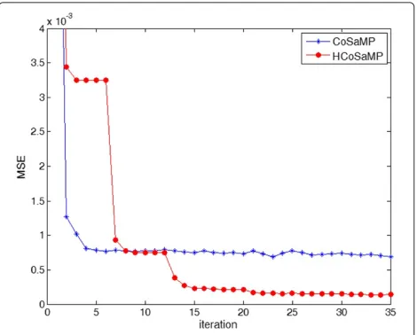
assumed K = 256. In Figure 2, we show the mean

squared error (MSE) on the reconstructed image obtained by the HCoSaMP at the different iterations. The hierar-chical approach of the HCoSaMP is well recognized in the plot of Figure 2, where the stepwise pattern of the MSE is due to the partial recovery of the DWT coeffi-cients over the increasing supports Li. The convergence

on the different layers can be clearly identified, as well as the floor achieved on each layer. To provide a compari-son, we have plotted also the MSE obtained by the classical

Figure 2CS acquisition of a spatially localized field with N₌4, 096,M₌900 andK₌256.MSE vs iterations obtained by the HCoSaMP and by the classical CoSaMP.

CoSaMP, detailed in [1]. The hierarchical structure of the HCoSaMP exploits the limited number of measure-ments by separately reconstructing the different layers, and it definitely outperforms the error floor of the classical reconstruction.

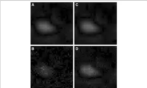
To visually confirm these results, we show in Figure 3 the reconstructed image obtained at convergence. For the sake of comparison, we report also the reconstruction results obtained by the model-based compressive sensing, described in [2], and by the work in [8]b_{. Both of these} works exploit the intrinsic structure of the DWT coeffi-cients to devise a reconstruction procedure which is able to obtain high reconstruction accuracy from a reduced number of CS measurements.

The HCoSaMP therefore well suites spatially localized images encountered in resource-constrained CS applica-tions, such as field monitoring in sensor network. For completeness sake, we also consider the case of natural image acquisition. We have considered the CS acquisi-tion of the fragment in Figure 1B extracted from the test image ‘Peppers’ withM = 1, 500 measurements and

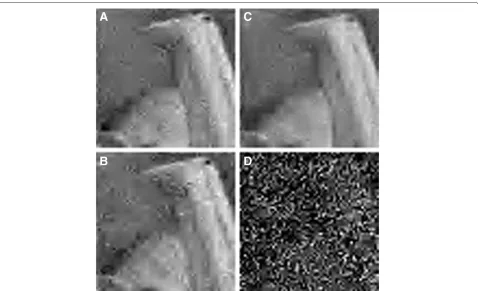
K = 1, 024. We show in Figure 4 the reconstruction

MSE obtained by HCoSaMP and CoSaMP, and in Figure 5 the reconstructed images obtained at convergence by the HCoSaMP, the model-based CS [2], the work in [8], and the classical CoSaMP. As for the case of spatially local-ized fields, inspection of Figures 4 and 5 confirms that the HCoSaMP still performs better than or equally to selected state-of-the-art approaches when compared on a fair basis. In particular, for fairness sake, it must be noticed that the HCoSaMP competitor [8] relies on spe-cific priors on the coefficients of a natural image in the

DWT domain. In order to employ sucha priori

Figure 3CS acquisition of a spatially localized field withN=4, 096,M=900 andK=256.Reconstructed image obtained by(A)the HCoSaMP,(B)the model-based CS [2],(C)the work in [8] and(D)the classical CoSaMP.

The herein presented HCoSaMP has the merit of relax-ing anya prioriassumption but the NAP property in the sparsity domain. In the following, we investigate the case of a texture image, where typical assumptions found in dealing with natural images do not hold, and we show that the HCoSaMP outperforms selected state-of-the-art

Figure 4CS acquisition of a natural image withN₌4, 096, M₌1, 500 andK₌1, 024.MSE vs iterations obtained by the HCoSaMP and by the classical CoSaMP.

works, due to its looser assumptions which best cope with application cases where approaches designed for natural image have poor performance.

5.2 Compressible signals in the GBT domain

The graph-based transform (GBT) has been recently introduced in the framework of video coding [16] to provide a novel representation domain which is able to efficiently capture image discontinuities. The GBT relies on an image-dependent basis suitably built to accom-modate for image boundaries and abrupt luminance dis-continuities; because of this peculiar structure, it has been employed in the framework of depth map cod-ing [21]. The GBT can be also applied as a sparsi-fying representation for texture images [9], which are hardly compressible in classical transformed domains such as the DWT or the discrete cosine transform (DCT) domains. Here, we show by numerical examples that tex-ture images satisfy the NAP in the GBT domain and are therefore viable of being reconstructed using the HCoSaMP.

Figure 5CS acquisition of a natural image withN=4, 096,M=1, 500 andK=1, 024.Reconstructed image obtained by(A)the HCoSaMP, (B)the model-based CS [2],(C)the work in [8] and(D)the classical CoSaMP.

This notwithstanding, the GBT, being strongly related to the image structure, can be applied in all those applica-tions where a class of images sharing the same structure can be identified. In these cases, in fact, the GBT basis may be built on a selected image, representative of the whole class, and can then be applied also to the other images in the class. This is indeed the case for texture image, where classes of images sharing the same structure can be easily found, and the GBT may be effectively employed to devise a sparsifying basis for CS acquisition.

Before turning to the presentation of numerical simu-lation results in this reference scenario, we give a brief sketch on the GBT basis construction. The interested reader can refer to [16] and [21] for more details. Given an

N pixel imagex, the GBT orthonormal basis is given by the eigenvectorsri,i=1,. . .,N, diagonalizing the matrix

Abuilt as follows:

A=diag ⎧ ⎨ ⎩

N

j=1

l0,j, N

j=1

l1,j,. . ., N

j=1

lN,j

⎫ ⎬ ⎭−L

whereLis a binaryN×N adjacency matrix whose ele-mentlu,vis set to 1 if the pixelsuandvare not separated

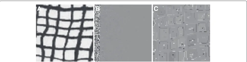
by an image edges, and it is set to 0 otherwise. In Figure 6, we show an example of a 64×64 fragment extracted from

the D104 Brodatz texture (available in [22]), along with its GBT representation and a selected vector from the GBT basis. Inspection of Figure 6 shows how the GBT domain is able to compactly represent the texture image; besides, the eigenvector in Figure 6C clearly confirms the strong bind among the GBT basis elements and the image structure.

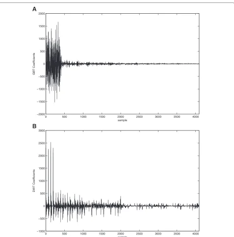
To show how the GBT provides a better basis to pro-vide compressibility for texture images, we plot in Figure 7 the coefficient vectors of GBT and DWT (the latter is obtained by the Daubechies wavelet transform) of the tex-ture D104 in Figure 6A. It easily recognized the higher compressibility attained in the GBT domain.

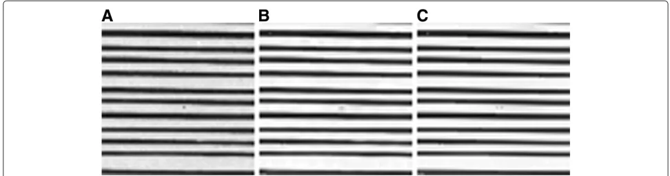
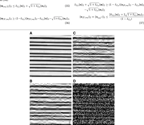
Besides being a suitable representation basis to devise a compressible representation for texture images, the GBT domain is also characterized by the NAP. To assess this property, we respectively show in Figure 8A a 64×64 pixel fragment cropped from the D49 Brodatz texture along with the reconstructed version obtained by retaining only the first 1/8 (Figure 8B) and 1/16 (Figure 8C) of the GBT coefficients.

Figure 6A 64×64 fragment from the D104 Brodatz texture with its GBT representation and a selected basis element.(A)Fragment cropped from the D104 Brodatz texture.(B)GBT of the fragment.(C)Example of an element of the GBT basis.

For the running of the HCoSaMP, we have considered the supportsLiconstituted by the first 1/256, 1/64, 1/16,

1/4 and 1/2 GBT coefficients.

To test the performance of the HCoSaMP, we have com-pressively sampled the D49 Brodatz texture in Figure 8A

with M = 2, 000 and K = 1, 024. In Figure 9, we

plot the MSE attained by the HCoSaMP and by the clas-sical CoSaMP. Results confirm the effectiveness of the HCoSaMP in hierarchically recovering the GBT coeffi-cients. Qualitative results are found in Figure 10 showing the results obtained by the HCoSaMP algorithm at dif-ferent iteration steps. In Figure 11, we also provide a comparison of the reconstructed images obtained by the different tested algorithms. Specifically, as for the case of natural and spatially localized images, we have compared the performance of the HCoSaMP with the model-based CS [2], with the approach in [8] and with the classical CoSaMP algorithm. Remarkably, since the structure of the GBT coefficients differs from the DWT one, state-of-the-art works relying on the DWT structure fail to attain satisfactory reconstruction quality. Still, a disserta-tion is in order. The work in [8] relies on the assumpdisserta-tion that the representation exhibits a tree structure such as the one characterizing the DWT coefficients; whenever this assumption fails to hold, as in the case of the GBT representation, the recovery exhibits poor performance. The work in [2] is more general and can accommo-date for different structures in the transformed domain. Here, we have employed the Matlab code provided by the authors in [23], designed for tree-structured signals; bet-ter results may be attained by adapting the model-based CS to the specific structure of the coefficients in the GBT domain.

We observe that the recovery of texture images from compressive sampling measurements is an open research challenge and could benefit from more complex texture generation models, as those envisaged for texture classifi-cation purposes [24,25]; the herein presented results pave the way for further studies on this issue.

6 Conclusion

In this paper, we have presented a reconstruction proce-dure, which we called HCoSaMP, for recovery of com-pressively sampled signals characterized by the so-called nested approximation property. This property can be found in a wide range of applications where other stronger hypotheses - e.g. tree coefficients’ structures - fail to hold. The convergence of the HCoSaMP procedure is analyt-ically demonstrated. Besides, the HCoSaMP procedure is validated by numerical simulation results and perfor-mance comparison with state-of-the-art reconstruction procedures. The adoption of the HCoSaMP is benefi-cial in resource-constrained applications where the cost of the measurements is high [6] and the number of col-lected measurements does not suffice for the CoSaMP procedure to converge. Finally, the herein presented anal-ysis draws a path towards hierarchical solution of differ-ent recovery algorithms for which robust convergence is guaranteed.

Endnotes

a_{The energy of the error vectore}

0is bounded by e02≤(1+δK)α12+ n2; as will be clarified in the following, such error, in the HCoSaMP convergence, plays much the same role played by the approximation error in the CoSaMP convergence on non-sparse, compressible signals.

b_{To implement the reconstruction algorithms}

described in [2] and in [8], we have employed the MatLab codes provided by the authors, available respectively in [23] and [26].

Appendix 1

Proof.(Proof of Lemma 4.1) Let us consider the setT=

∪supp(α(₀j−1)), as in Algorithm 1, and let us define

b|T =†_|Ty=†_|T(α0+e0)

b_|TC =0.

0 500 1000 1500 2000 2500 3000 3500 4000 −2000

−1500 −1000 −500 0 500 1000 1500 2000

sample

GBT Coefficients

0 500 1000 1500 2000 2500 3000 3500 4000

−1000 −500 0 500 1000 1500 2000 2500 3000

sample

DWT Coefficients

A

B

Figure 7Coefficient vectors of GBT and DWT.(A)GBT vector of the D104 fragment in Figure 6.(B)DWT vector of the D104 fragment in Figure 6.

Within these settings, b represents the LS estimate of the signal samples evaluated on the supportT. We prove that the energy of the estimation error is upper bounded by a term proportional to the energy of the signal α₀ over the support TC and by a term proportional to the measurement noise energy:

α0−b2≤ α0|TC

1+ δL0 1−δ_L0 +

e0

1−δ_L0. (27)

Let us start by noting that the set T is defined as the union of two proper subsets ofL0, so that its cardinality is upper bounded byL0. Keeping this in mind, let us con-sider the Euclidean distance betweenb andα₀. We can write

α0−b2=α0|T+α0|TC−b2≤ α0|TC2+ α0|T−b|T2,

=α_0|TC2+α0|T−†_|Tα0|T+α_0|TC+e02.

Figure 8NAP property for texture images in the GBT domain.(A)Original fragment of the D49 Brodatz texture.(B)Image obtained by retaining only 1/8 of the GBT coefficients.(C)Image obtained by retaining only 1/16 of the GBT coefficients.

Simple algebra leads to

α0−b2≤ α0|TC₂+ †_|T

α_0|TC+n

2, ≤ α_0|TC₂+ †_|Tα_0|TC₂+ †_|Te₀₂.

(29)

Finally, noting that|T ∪supp(α0)| ≤ L0, we come up with the following upper bound (cfr. also Lemmas 1 to 3 in [1]):

α₀−b2≤ α0|TC

1+ δL0 1−δ_L0 +

e0

1−δ_L0. (30)

Under the assumption thatδ_L0 = 0.1, the expression in (13) is evaluated as follows

α0−b2≤1.112α0|TC₂+1.06e₀₂. (31)

This concludes the proof.

Figure 9CS acquisition of D49 texture withN=4, 096, M=2, 000 andK=1, 024.MSE vs iterations obtained by the HCoSaMP and by the classical CoSaMP.

Appendix 2

Proof.(Proof of Lemma 4.2) Let us recall the starting positions as found in (16):

s=α0−α0(j) (Signal not yet recovered at iterationj)

r=y−α₀(j)=s+e0 (Residual at iterationj- it is just a CS acquisition of the signals)

u=∗r (Proxy at iterationj)

ω0=L0∩supp(u2K)

(32)

Let us first denote thatα₀is confined toL0by definition and thatα₀(j)is confined toL0by construction. Then, the signalsexhibits at mostL0nonzero coefficients. Then, let us define =supp(s). Assis at mostL0sparse, then we have| | ≤ L0. Now, because of the NAP property (cfr. [2]), the setω0is the one collecting the indices providing the support of the best approximation ofuwithin the set L0, so that, following the clear guidelines posed in [1], we can write the following derivations:

u−u|ω022≤ u−u 22 (33)

n

u(n)−uω0(n)

2_≤

n

u(n)−u| (n)2

n

u(n)−uω0(n)

2_≤

n

(u(n)−u (n))2

n∈ω0

(u(n))2≥

n∈

(u(n))2

n∈ω₀

n∈/ω₀

(u(n))2≥

n∈

n∈/ω₀

(u(n))2

n∈ω0\

(u(n))2≥

n∈ \ω0 (u(n))2

u|ω0\ 2

2≥ u| \ω0 2 2.

(34)

Figure 10CS acquisition of D49 texture withN=4, 096,M=2, 000 andK=1, 024.Reconstructed image obtained by the HCoSaMP after(A) 5 iterations,(B)10 iterations and(C)20 iterations.

compactness, we derive the following bounds on the terms in (34):

u|ω0\ 2≤δL0s2+

1+δ_L0e02 (35)

u| \ω02≥(1−δL0)s| \ω02−δL0s2−

1+δ_L0e02. (36)

By injecting (35) and (36) in (34), we come up withc

δ_L0s2+

1+δ_L0n2≥(1−δL0)s|R\ω02−δL0s2 −1+δ_L0e02

s| \ω02= s|ω0C2≤

2δ_L0s2+2

1+δ_L0e02 (1−δ_L0)

(37)

where we have sets| \ω0 = s|ω0C due to the fact that

The authors declare that they have no competing interests.

Received: 30 December 2013 Accepted: 14 May 2014 Published: 31 May 2014

References

1. D Needell, JA Tropp, CoSaMP: Iterative signal recovery from incomplete and inaccurate samples. Appl. Comput. Harmonic Anal.26, 301–321 (2008)

2. RG Baraniuk, V Cevher, MF Duarte, C Hegde, Model-based compressive sensing. IEEE Trans. Inform Theory.56(4), 1982–2001 (2010)

3. S Colonnese, R Cusani, S Rinauro, G Scarano, Bayesian prior for reconstruction of compressively sampled astronomical images, in4th European Workshop on Visual Information Processing(EUVIP 2013 Paris, June 2013)

4. RG Baraniuk, C Hegde, Sampling and recovery of pulse streams. IEEE Trans. Signal Process.59(4), 1505–1517 (2011)

5. Y Eldar, M Mishali, Robust recovery of signals from a union of subspaces. IEEE Trans. Inf. Theory.55, 5302–5316 (2009)

6. S Colonnese, R Cusani, S Rinauro, G Ruggiero, G Scarano, Efficient compressive sampling of spatially sparse fields in wireless sensor networks. EURASIP J. Adv. Signal Process.136, 1–19 (2013)

7. F Fazel, M Fazel, M Stojanovic, Random access compressed sensing for energy-efficient underwater sensor networks. IEEE J. Selected Areas Commun.29(8), 1660–1670 (2011)

8. L He, L Carin, Exploiting structure in wavelet-based Bayesian compressive sensing. IEEE Trans. Signal Process.57(9), 3488–3497 (2009)

9. S Colonnese, S Rinauro, K Mangone, M Biagi, R Cusani, G Scarano, Reconstruction of compressively sampled texture images in the graph-based transform domain, inIEEE International Conference on Image Processing (ICIP)(Paris, 27–30 October 2014)

10. EJ Candes, T Tao, Decoding by linear programming. IEEE Trans. Inform. Theory.51, 4203–4215 (2005)

11. M Rudelson, R Vershynin, On sparse reconstruction from Fourier and Gaussian measurements. Comm. Pure Appl. Math.61, 1025–1045 (2008) 12. R Vershynin, On the role of sparsity in Compressed Sensing and Random

matrix theory, CAMSAP’09, in3rd International Workshop on

Computational Advances in Multi-Sensor Adaptive Processing(Aruba, Dutch Antilles, 13–16 December 2009)

13. B Bah, J Tanner, Improved bounds on restricted isometry constants for Gaussian matrices. J. SIAM J. Matrix Anal. Appl.31(5), 2882–2898 (2010) 14. B Mailhe, B Sturm, MD Plumbley, Behavior of greedy sparse

representation algorithms on nested supports, inProceedings of the 2013 IEEE International Conference on Acoustics, Speech and Signal Processing (ICASSP)(Vancouver, Canada, 26–31 May 2013)

15. Y Liu, DA Pados, Decoding of framewise compressed-sensed video via inter-frame total variation minimization. SPIE J. Electron. Imaging Special Issue Compressive Sensing Imaging.22, 1–8 (2013)

16. S Lee, A Ortega, Adaptive compressive sensing for depthmap

compression using graph-based transform, inProceedings of International Conference on Image Processing (ICIP) 2012(Orlando, FL, USA, 30 September to 3 October 2012)

17. HL Yap, A Eftekhari, MB Wakin, CJ Rozell, The restricted isometry property for block diagonal matrices, in45th Annual Conference on Information Sciences and Systems (CISS)(IEEE Baltimore, 23 Mar to 25 Mar 2011) 18. A Eftekhari, HL Yap, CJ Rozell, MB Wakin, The restricted isometry property

for random block diagonal matrices (2012). arXiv preprint arXiv:1210.3395

19. D Needell, R Ward, Stable image reconstruction using total variation minimization. SIAM J. Imaging Sci.6.2(2013), 1035–1058 (2013) 20. Jet Propulsion Laboratory, JPL’s OurOcean portal. http://ourocean.jpl.

nasa.gov. Accessed 26 May 2014

21. G Cheung, W-S Kim, A Ortega, J Ishida, A Kubota, Depth map coding using graph based transform and transform domain sparsification, in

Proceedings of International Workshop on Multimedia Signal Processing (MMSP)(Hangzhou, China, 17–19 October 2011)

22. T Randen, Brodatz textures. http://www.ux.uis.no/~tranden/brodatz.html. Accessed 26 May 2014

23. RG Baraniuk, V Cevher, MF Duarte, C Hegde, Model-based Compressive Sensing Toolbox v1.1. http://dsp.rice.edu/software/model-based-compressive-sensing-toolbox. Accessed 26 May 2014

24. P Campisi, A Neri, G Scarano, Reduced complexity modeling and reproduction of colored textures. IEEE Trans. Image Process.9(3), 510–518 (2000)

25. P Campisi, S Colonnese, G Panci, G Scarano, Reduced complexity rotation invariant texture classification using a blind deconvolution approach. IEEE Trans. Pattern Anal. Mach. Intell.28(1), 145–149 (2006)

26. L Carin, S Ji, Y Xue, Bayesian Compressive Sensing code. http://people.ee. duke.edu/~lcarin/BCS.html. Accessed 25 May 2014

doi:10.1186/1687-6180-2014-80

Cite this article as:Colonneseet al.:Hierarchical CoSaMP for compressively sampled sparse signals with nested structure.EURASIP Journal on Advances in Signal Processing20142014:80.

Submit your manuscript to a

journal and benefi t from:

7Convenient online submission

7Rigorous peer review

7Immediate publication on acceptance

7Open access: articles freely available online

7High visibility within the fi eld

7Retaining the copyright to your article