Maximum MIMO System Mutual Information with Antenna Selection and Interference

Maximum MIMO System Mutual Information

with Antenna Selection and Interference

Rick S. Blum

Department of Electrical and Computer Engineering, Lehigh University, Bethlehem, PA 18015-3084, USA Email:[email protected]

Received 31 December 2002; Revised 13 August 2003

Maximum system mutual information is considered for a group of interfering users employing single user detection and antenna selection of multiple transmit and receive antennas for flat Rayleigh fading channels with independent fading coefficients for each path. In the case considered, the only feedback of channel state information to the transmitter is that required for antenna selection, but channel state information is assumed at the receiver. The focus is on extreme cases with very weak interference or very strong interference. It is shown that the optimum signaling covariance matrix is sometimes different from the standard scaled identity matrix. In fact, this is true even for cases without interference if SNR is sufficiently weak. Further, the scaled identity matrix is actually that covariance matrix that yields worst performance if the interference is sufficiently strong.

Keywords and phrases:MIMO, antenna selection, interference, capacity.

1. INTRODUCTION

Multiple-input multiple-output (MIMO) channels formed using transmit and receive antenna arrays are capable of pro-viding very high data rates [1,2]. Implementation of such systems can require additional hardware to implement the multiple RF chains used in a standard multiple transmit and receive antenna array MIMO system. Employing antenna se-lection [3,4] is one promising approach for reducing com-plexity while retaining a reasonably large fraction of the high potential data rate of a MIMO approach. One antenna is se-lected for each available RF chain. In this case, only the best set of antennas is used, while the remaining antennas are not employed, thus reducing the number of required RF chains. For cases with only a single transmit antenna where standard diversity reception is to be employed, this approach, known as “hybrid selection/maximum ratio combining,” has been shown to lead to relatively small reductions in performance, as compared with using all receive antennas, for considerable complexity reduction [3,4]. Clearly, antenna selection can be simultaneously employed at the transmitter and at the re-ceiver in a MIMO system leading to larger reductions in com-plexity.

Employing antenna selection both at the transmitter and the receiver in a MIMO system has been studied very recently [5,6,7]. Cases with full and limited feedback of information from the receiver to the transmitter have been considered. The cases with limited feedback are especially attractive in that they allow antenna selection at the transmitter without requiring a full description of the channel or its eigenvector

decomposition to be fed back. In particular, the only infor-mation fed back is the selected subset of transmit antennas to be employed. While cases with this limited feedback of infor-mation from the receiver to the transmitter have been studied in these papers, each assume that the transmitter sends a dif-ferent (independent) equal power signal out of each selected antenna. Transmitting a different equal power signal out of each antenna is the optimum approach for the case where se-lection is not employed [8] but it is not optimum if antenna selection is used. The purpose of this paper is to find the op-timum signaling. This problem is still unsolved to date. For simplicity, we ignore any delay or error that might actually be present in the feedback signal. We assume the feedback signal is accurate and instantly follows any changes in the environ-ment.

Consider a system where cochannel interference is present fromL−1 other users. We focus on theLth user and assume each user employs nt transmit antennas andnr

re-ceive antennas. In this case, the vector of rere-ceived complex baseband samples after matched filtering becomes

yL=ρLHL,LxL+ L−1

j=1

ηL,jHL,jxj+n, (1)

where HL,j and xj represent the normalized channel

ma-trix and the normalized transmitted signal of user j, respec-tively. The signal-to-noise ratio (SNR) of user Lis ρL and

of the interfering signalsxj, j = 1,. . .,L−1, are unknown

to the receiver and we model each of them as being complex Gaussian distributed, the usual form of the optimum signal in MIMO problems. Then if we condition onHL,1,. . .,HL,L,

the interference-plus-noise from (1),Lj=1−1√ηL,jHL,jxj+n,

is complex Gaussian distributed with the covariance matrix

RL=

L−1

j=1ηL,jHL,jSjHHL,j+Inr, whereSjdenotes the

covari-ance matrix ofxjandInr is the covariance matrix ofn.

Un-der this conditioning, the interference-plus-noise is whitened by multiplyingyLbyR−1L /2. After performing this

multiplica-tion, we can use results from [2,8,9] (see also [10, pp. 12–23, pp. 250,256]) to express the ergodic mutual information be-tween the input and output for the user of interest as in the following:

IxL;

yL,H

=Elog₂detInr+ρL

R−1L /2HL,L

SL

R−1L /2HL,L

H

=Elog₂detInr+ρLHL,LSLH H L,LR−1L

(2)

(H reminds us of the assumed model forHL,1,. . .,HL,L). In

(2), the identity det (I+AB)=det (I+BA) was used. If we wish to compute total system mutual information, we should findS1,. . .,SLto maximize

ΨS1,. . .,SL

=

L

i=1 Ixi;

yi,H

=

L

i=1 E

  log2

 _det



_{Inr+ρiHi,iSiH}H i,i

×

Inr+ L

j=1,j=i

ηi,jHi,jSjHHi,j

−1      .

(3)

Now, assume that each receiver selectsnsr < nrreceive

an-tennas andnst< nttransmit antennas based on the channel

conditions and feeds back the information to the transmit-ter.1 _{Then the observations from the selected antennas} fol-low the model in (1) withntandnrreplaced bynstandnsr,

respectively, andHi,jreplaced byH˜i,j. The matrixH˜i,jis

ob-tained by eliminating those columns and rows ofHi,j

corre-sponding to unselected transmit and receive antennas. Thus we can writeH˜i,j=g(Hi,j), where the functiongwill choose

˜

Hi,j to maximize the instantaneous (and thus also the

er-godic) mutual information (or some related quantity for the signaling approach employed). In order to promote brevity, we will restrict attention in the rest of this paper to the case wherenst =nsr so we will only use the notation fornst. We

note that the majority of the results given carry over imme-diately for the case ofnst=nsr, and since this will be obvious

in these cases, we will not discuss this further.

It is important to note that we restrict attention to nar-rowband systems using single user detection, equal power

1_{The case where each user employs a differentnstandnsris also easy to} handle.

(constant over time) for each user, and fixed definitions of the transmitting and receiving users. Future extensions which remove some assumptions are of great interest. How-ever, as we will show, these assumptions lead to interesting closed form results which we believe give insight into the fun-damental properties of MIMO with antenna selection.

InSection 2, we give a general discussion and some use-ful relationships used to study the convexity and concavity properties of the system mutual information. In Section 3, we study cases with weak interference. We follow this, in Section 4, with our results for strong interference. The results in Sections3and4are general for anynst =nsr,nt,nr, and

L.Section 5is devoted to numerical studies for the particu-lar case ofnr =nt =8,nsr =nst = L= 2 to illustrate the

agreement with the theory from Sections3and4. The results inSection 5also show that our asymptotic results give use-ful information for nonasymptotic cases as well. The paper concludes withSection 6.

2. GENERAL ANALYSIS OF SYSTEM MUTUAL INFORMATION

Clearly, the nature of the functional2_{Ψ(S1,. . .,S}

L) will

de-pend on the SNRsρi,i =1,. . .,L, and the INRsηi,j,i,j =

1,. . .,L,i=j. This can be seen by considering the convexity and the concavity ofΨ(S1,. . .,SL) as a function ofS1,. . .,SL.

Towards this goal, we define a general convex combination of two possible solutions (S1,. . .,SL) and (ˆS1,. . ., ˆSL) as follows:

_¯

S1,. . ., ¯SL

=(1−t)S1,. . .,SL

+tSˆ1,. . ., ˆSL

=S1,. . .,SL

+tSˆ1,. . ., ˆSL

−S1,. . .,SL

=S1,. . .,SL

+tS1,. . .,SL

(4)

for 0≤t≤1 a scalar. ThenΨ(S1,. . .,SL) is a convex function

of (S1,. . .,SL) if [12]

d2 dt2Ψ

_¯

S1,. . ., ¯SL

≥0 ∀_S¯_{1,. . ., ¯SL. (5)} Similarly,Ψ(S1,. . .,SL) is a concave function of (S1,. . .,SL) if

d2 dt2Ψ

_¯

S1,. . ., ¯SL

≤0 ∀_S¯_{1,. . ., ¯SL. (6)} There are several useful known relationships for the deriva-tive of a function of a matrixΦwith respect to a scalar pa-rametert. In particular, we note that [13, Appendix A, pp. 1342, 1345, 1349, 1351, 1359, 1401]

d dtln

det (Φ)=trace Φ−1 !

d dtΦ

"# ,

d dtΦ

−1_{= −Φ}−1!d dtΦ

" Φ−1_.

(7)

Assuming selection is employed, we can use (3) and (7) to find (interchanging a derivative and an expected value)

d

A second derivative yields

d2

3. OPTIMUM SIGNALING FOR WEAK INTERFERENCE We can use (12) to investigate convexity and concavity for any particular set of SNRsρi,i=1,. . .,L, and INRsηi,j,i,j=

1,. . .,L,i= j. We investigate extreme cases, weak or strong interference, to gain insight. The following lemma considers the case of very weak interference.

Lemma 1. Assuming sufficiently weak interference, the best (S1,. . .,SL)(that maximizes the ergodic system mutual infor-mation) must be of the form

_¯

Outline of the proof. For the case of very weak interference,

we ignore terms which are multiples of ηi,j (essentially, we

setηi,j →0 fori=1,. . .,L, j =1,. . .,L, and j =i) and we

diagonal matrices with nonnegative entries. Define A = ρiHi,iSiHHi,i and note that AH = A due to Si being a

difference of two covariance matrices (easy to see using

UΛUH_{expansion for each covariance matrix). Thus the trace}

in (15) can be written as trace[U(Ω)2_UH_AU(Ω)2_UH_{A] =}

trace[UΩUH_AU(Ω)2_UH_AUΩUH_{] = trace[BB}H_{] since}

trace [CD] = trace [DC] [13]. We see trace[BBH_{] must be}

nonnegative since the matrix inside the trace is nonnegative-definite so that (15) implies that Ψ(S1,. . .,SL) is concave.

This will be true for sufficiently small ηi,j,i,j = 1,. . .,L,

i = j, relative to ρi, i = 1,. . .,L. To recognize the

sig-nificance of the concavity, we note that given any permu-tation matrix Π, we know [8] that H˜i,j has the same

dis-tribution as H˜i,jΠ (switching the ordering or names of

se-lected antennas cannot change the physical problem), so Ψ(ΠS1ΠH,. . .,ΠSLΠH)=Ψ(S1,. . .,SL). Let

Πdenote the

sum over all the different permutation matrices and let N denote the number of terms in the sum. From concavity, Ψ((1/N)_ΠΠS1ΠH,. . ., (1/N)

ΠΠSLΠH)≥Ψ(S1,. . .,SL)

[8] which implies that the optimum (S1,. . .,SL) must be of

the form such that it is invariant to transforms by permu-tation matrices. This implies that the best (S1,. . .,SL) must

be of the form given in (14). We refer the interested reader to [14] for a rigorous proof of this (taken from a single user case).

Before considering specific assumptions on the SNR, we note the similarity of (14) to (4) with (S1,. . .,SL) =

(1/nst)(Onst,. . .,Onst), (ˆS1,. . ., ˆSL)=(1/nst)(Inst,. . .,Inst), and

t=γ1= · · · =γL.

Small SNR

Thus we have determined the best signaling except for the unknown scalar parametersγ1,. . .,γLwhich we now

inves-tigate. Generally, the best approach will change with SNR. First, consider the case of weak SNR for which the following lemma applies (recall we have now already focused on very weak or no interference).

Lemma 2. Leth(p,˜ p)i,j denote the (i,j)th entry of the

weak interference and sufficiently weak SNR,

where thenst×nstmatrix can be explicitly written as

Inst−Onst=

Explicitly carrying out the operations in (18) gives (16).

Notice that without selection (in this caseH˜p,p =Hp,p),

the quantity in (16) becomes zero under the assumed model for Hp,q (i.i.d complex Gaussian entries). Thus selection

turns out to be an important aspect in the analysis. The fol-lowing lemmas will be used with the result in Lemma 2to develop the main result of this section.

Lemma 3. Leth(p,˜ p)i,j denote the(i,j)th entry of the

ma-trixH˜p,pand defineS¯1,. . ., ¯SLfrom(14). Assuming sufficiently

weak interference and sufficiently weak SNR,

Ψ_S¯_{1,. . ., ¯SL}

Outline of the proof. Consider annst×nst nonnegative

def-inite matrix A and let λ1(A),. . .,λnst(A) denote the eigen-assume that selection is employed. Thus we consider the re-sultingΨas a function of (γ1,. . .,γL) and we see

Note that thenst×nstmatrix can be explicitly written as

Lemma 4. Assuming sufficiently weak interference and suffi -ciently weak SNR, the antenna selection that maximizes the er-godic system mutual information will make

E

Outline of the proof. First, consider the antenna selection

ap-proach for thepth link which maximizes the ergodic system mutual information in (20) whenγp=1 in (14). Thus the

se-lection approach will maximize the quantity in thepth term in the first sum in (20) whenγp = 1 by selecting antennas

for each set of instantaneous channel matrices to make the terms inside the expected value as large as possible. It is im-portant to note that the choice (ifγp =1) depends only on

the squared magnitude of elements of the channel matrices. If we use this selection approach whenγp =1, then the

terms multiplied by (1−γp) in (20) will be averaged to zero

due to the symmetry in the selection criterion. To see this, first note that the contribution to the ergodic mutual infor-mation due to thepth term is

times the constantρp/nstln (2). In (24),

fh(p,p)1,1,...,h(p,p)nt,nr

h(p,p)1,1,. . .,h(p,p)nt,nr

(25)

is the probability density function of the channel coefficients prior to selection, the integral is over all values of the argu-ments and the selection ruleH˜ =g(H) is important in de-termining the integrand. If the optimum selection rule for (20) withγp =1 will select a particular set of transmit and

receive antennas for a particular instance of h(p,p)1,1,. . ., h(p,p)nt,nr, then due to symmetry, this same selection will

also occur several more times as we run through all the pos-sible values of h(p,p)1,1,. . .,h(p,p)nt,nr. Thus assume that

terms with|h(p,p)ˆijˆ|2=aand|h(p,p)ˆijˆ|2=bin (20) with γp=1 are large enough to cause the corresponding antennas

to be selected by the selection criterion trying to maximize (20) withγp = 1 for some set ofh(p,p)11,. . .,h(p,p)nst,nst.

Then due to the symmetry,

_˜

h(p,p)∗i j, ˜h(p,p)i j=√aejφa_,bejφb_,

_˜

h(p,p)∗i j, ˜h(p,p)i j=√aejφa_,−_bejφb_,

_˜

h(p,p)∗i j, ˜h(p,p)i j=−√aejφa_,bejφb_,

h(p,p)∗i j,h(p,p)i j=−√aejφa_,−_bejφb

(26)

will all appear in (24). Since each of these four possible val-ues appear for four equal area (actually probability) regions in channel coefficient space, a complete cancellation of these terms results in (24). In fact, this leads to (24) averaging to zero. Thus if we use the selection approach that will maxi-mize (20) withγp=1, this is the best we can do.

However, ifγp = 1, we can do better. Due to the cross

terms in (20) in the term multiplied by (1−γp), we can

use selection to do better by modifying the selection ap-proach. To understand the basic idea, letH˜denote the ma-trix H˜p,p for a particular selection of antennas andH˜

de-note the same quantity for a different selection of anten-nas. Now consider two selection approaches which are the same except the second approach will choose H˜ in cases where

nst

i=1

nst

j=1 **_H˜

i j|2= nst

i=1

nst

j=1 **_H˜

i j|2,

nst

i=1

nst

j=1

nst

j_=1,j₌j

˜

Hi jH˜i j∗ >0,

(27)

and (in the sum, both a term and its conjugate appear, giving a real quantity)

nst

i=1

nst

j=1

nst

j_=1,j₌j

˜

Hi jH˜i j∗ <0. (28)

Assume the first selection approach is the one trying to

max-imize (20) withγp=1 so it will just select randomly if

nst

i=1

nst

j=1 **_H˜

i j**

2 =

nst

i=1

nst

j=1 **_H˜

i j**

2

, (29)

since it ignores the cross terms in its selection.

From (20), the second selection approach will give larger instantaneous mutual information for each event where the selection is different. Since the probability of the event that makes the two approaches different is greater than zero un-der our assumed model, then the second antenna selec-tion approach will lead to improvement (if γp = 1) and

it will do this by making the term multiplied by (1−γp)

in (20) positive. Clearly the optimum selection scheme will be at least as good or better, so it must also give improve-ment by making the term multiplied by (1 −γp) in (20)

positive.

We are now ready to give the main result of this section.

Theorem 1. Assuming sufficiently weak interference, suffi -ciently weak SNRs, and optimum antenna selection, the best (S1,. . .,SL)(that maximizes the ergodic system mutual infor-mation) uses

_¯

S1,. . ., ¯SL

= 1

nst

Onst,. . .,Onst

. (30)

Outline of the proof. The assumption of weak SNRs

implies that ρp is small for all 1 ≤ p ≤ L. In

this case, optimum selection will attempt to make E{nst

i=1 nst

j=1 nst

j_=1,j=jh˜∗(p,p)i,jh(p,˜ p)i,j} as large as possible as shown in Lemma 3. Lemma 4 builds on Lemma 3 to show that optimum selection can always make E{nst

i=1 nst

j=1 nst

j_=1,j=jh˜∗(p,p)i,jh(p,˜ p)i,j} positive. Lemma 2 shows that (d/dγp)Ψ is directly proportional to

the negative of E{nst i=1

nst j=1

nst

j_=1,j₌jh˜∗(p,p)i,j˜h(p,p)i,j} which the selection is making positive and large. Thus it follows that (d/dγp)Ψis always negative which implies that

the best solution employsγp = 0 since any increase in γp

away fromγp = 0 causes a decrease inΨ. Sinceρp is small

for allp, the theorem follows.

Large SNR

Now consider the case of large SNR, where the following the-orem applies.

Theorem 2. Assuming sufficiently weak interference, suffi -ciently large SNRs, and optimum antenna selection, the best (S1,. . .,SL)(that maximizes the ergodic system mutual infor-mation) uses

_¯

S1,. . ., ¯SL

= 1

nst

Inst,. . .,Inst

Outline of the proof. Asserting the weak interference, large SNR assumption in (8) gives

Q−1_i d

the interference is very weak, the best signaling uses (14) with γp=1. Since this is true for allp, the theorem follows.

As a further comment onTheorem 2, we note that the proof makes it clear that ifρpis large only for certainp, then

γp =1 for thoseponly. Likewise, it is clear fromTheorem 1

that ifρpis small only for certainp, thenγp =0 for thosep

only. Of course, this assumes weak interference. Thus we can image a case where the best signaling usesγp=1 for somep

andγp=0 for somep=pwith proper assumptions on the correspondingρp,ρp. One can construct similar cases where only some of theηi,j are small and easily extend the results

given here in a straight forward way.

4. STRONG INTERFERENCE

Now consider the other extreme of dominating interference whereηi,j,i = 1,. . .,L, j = 1,. . .,L, is large (compared to

ρ1,. . .,ρL). The following lemma addresses the worst

signal-ing to use.

Lemma 5. Assuming sufficiently strong interference, the worst (S1,. . .,SL)(that minimizes the ergodic system mutual infor-mation) must be of the form

_¯

Outline of the proof. Providedηi,jis sufficiently large, we can

approximate (9) as

ond term inside the trace in (12) depends inversely onη2

i,j

so that the first term dominates for large ηi,j. Further, we

can interchange the expected value and the trace in (12) so we are concerned with the expected value of (13). Now note that the first term in (13) consists of the product of a term

A=_H˜_i,iS

iH˜Hi,iand another term depending onH˜i,jforj=i.

Now consider the expected value of (13) computed first as an expected value conditioned on{_H˜_{i,j, j=i}and then this}

ex-pected value is averaged over{_H˜_{i,j, j=i}. Now note that the}

conditional expected value ofAbecomes the zero matrix.3 Thus the contribution from the first term in (13) averages to zero so that

which is nonnegative. To see this, we can use a few of the same simplifications used previously. Ex-pand the nonnegative definite matrices 2ρiH˜i,iS¯iH˜Hi,i

and (L_j=1,j=iηi,jH˜i,jS¯jH˜Hi,j)−1 using the unitary

ma-trix/eigenvalue expansions as done after (15). Then the matrix inside the expected value in (36) can be factored

3_RecallS

into BBH _{after manipulations similar to those used after}

(15). Thus Ψ(S1,. . .,SL) is convex. Thus using the same

permutation argument as used for the weak interference case, the result stated in the theorem follows.

The following theorem builds onLemma 5to specify the exactγ1,. . .,γLgiving worst performance.

Theorem 3. Assuming sufficiently strong interference and

opti-mum antenna selection, the worst(S1,. . .,SL)(that minimizes

the ergodic system mutual information) uses

_¯

S1,. . ., ¯SL

= 1

nst

Inst,. . .,Inst

. (37)

Outline of the proof. Consider Ψ(S1,. . .,SL) for (S1,. . .,SL)

of the form given byLemma 5which is (from (2) and (3))

ΨS1,. . .,SL

=

L

i=1

Elog₂detInst+ρiH˜i,iSiH˜ H i,iR−1i

≈

L

i=1 ρiE

traceH˜i,iSiH˜Hi,iR−1i

= 1

nstln (2) L

p=1 ρp

×E &_nst

i=1

nst

j=1

**_h(p,ˆ _p)

i,j**2

+1−γp

nst

i=1

nst

j=1

nst

j_=1,j=j ˆ

h∗(p,p)i,jh(p,ˆ p)i,j '

,

(38)

where the first simplification follows from largeηi,jand the

same simplifications used in (21). The second simplification follows from those in (20) but now ˆh(p,p)i,j denotes the

(i,j)th entry of the matrixR−1/2

p H˜p,p. Now note that antenna

selection will attempt to make the second term in the last line of (38), which multiplies the positive constant 1−γp, as large

and positive as it possibly can. In fact, it is easy to argue that antenna selection can always make this term positive as done previously for (20). We skip this since the problems are so similar. Thus we see that the best performance for (S1,. . .,SL)

of the form given byLemma 5must be obtained forγp =0

and the worst performance must occur atγp =1. Since this

is true for allp, the result in the theorem follows.

The result inTheorem 3tells us that the best signaling for cases without interference and selection is the worst for strong interference and selection. It appears that the best sig-naling for (S1,. . .,SL) of the form given byLemma 5(see the

discussion inTheorem 3) may be the best signaling overall. However, it appears difficult to show this generally.

The following intuitive discussion gives some further in-sight. Due to convexity, the best performance will occur at a point as far away from the point giving worst performance

(S1,. . .,SL)=(1/nst)(Inst,. . .,Inst) as possible (recall that the

γ1= · · · =γL=1 point gives the worst performance). Thus

the best performance occurs for a point on the boundary of our space of feasible (S1,. . .,SL) and this point must be as far

away from the point giving the worst performance as possi-ble. One such point is (S1,. . .,SL)=(1/nst)(Onst,. . .,Onst). It

can be shown generally (for anynst) that this solution is the

farthest from (S1,. . .,SL) = (1/nst)(Inst,. . .,Inst) (Frobenius

norm). This follows because (1/nst)Onst is the farthest from

(1/nst)Inst. Note thatSwith one entry of 1 and the rest zero is

equally far from (1/nst)Instbut numerical results in some

spe-cific cases indicate that the rate of increase in this direction is not as great as the rate of increase experienced by mov-ing along the line (S1,. . .,SL)=γ(1/nst)(Inst,. . .,Inst) + (1−

γ)(1/nst)(Onst,. . .,Onst) away fromγ=1 towardsγ=0.

5. NUMERICAL RESULTS FORnst=nsr=L=2,

nt=nr=8

Consider the case of nst = nsr = L = 2, nt = nr = 8,

η1,2 = η2,1 = η, andρ1 =ρ2 =ρand assume that the op-timum antenna selection (to optimize system mutual infor-mation) is employed. First consider the case of no interfer-ence and assume a set of covariance matrices of the form (S1,S2) = γ(1/2)(I2,I2) + (1−γ)(1/2)(O2,O2). Thus since ρ1=ρ2=ρandη1,2=η2,1=η, we setγ1=γ2=γ.Figure 1 shows a plot of theγgiving the largest mutual information versus SNR, for SNR (ρ) ranging from−10 dB to +10 dB. We see that the best performance for very smallρis obtained for γ=0 which is in agreement with our analytical results given previously. For largeρ, the best signaling usesγ=1 which is also in agreement with our analytical results given previously. Figure 1shows that the switch from whereγ=0 is optimum to where γ = 1 is optimum is very rapid and occurs near ρ= −3 dB.

Now consider cases with possible interference. Again consider the case of nst = nsr = L = 2, nt = nr = 8,

η1,2=η2,1=η, andρ1 =ρ2 =ρand assume that the opti-mum antenna selection (to optimize system mutual informa-tion) is employed. To simplify matters, we constrainS1=S2 in all cases shown. First we considered three specific signaling covariance matrices which are

S1=S2=     1 2 0 0 1 2    ,

S1=S2=     1 2

1 2 1 2

1 2    ,

S1=S2=

1 0 0 0

.

(39)

1 0.9 0.8 0.7 0.6 0.5 0.4 0.3 0.2 0.1 0

γ

−10 −8 −6 −4 −2 0 2 4 6 8 10 SNR

Figure 1: Optimumγ versusρ1 = ρ2 = SNR for cases with no interference and nst = nsr = 2,nt = nr = 8. Note thatγ = 0 is the best for−10 dB < SNR< −3 dB andγ =1 is the best for −2 dB<SNR<10 dB.

10 8 6 4 2 0 −2

−4 −6 −8 −10

SNR

(dB)

−10 −8 −6 −4 −2 0 2 4 6 8 10 INR (dB)

0

0

0

[10; 00] worst

0.5∗[10; 01] worst

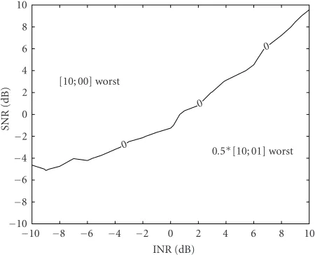
Figure2: The worst signaling (of the three approaches) versus SNR and INR fornst=nsr =L=2,nt=nr =8,ρ1=ρ2=SNR, and η1,2=η2,1=INR.

results given in Sections3and4of this paper for weak and strong interference and SNR. Figure 2shows the worst sig-naling we found versus SNR and INR forρ1 = ρ2 = SNR and η1,2 = η2,1 = INR. For large INR,Figure 2 indicates thatS1 = S2 = (1/2)I2 leads to worst performance which is in agreement with our analytical results given previously. Figure 2also shows that eitherS1 =S2 =(1/2)I2(for weak SNR) or (for large SNR)S1=S2with only one nonzero entry (a one which must be along the diagonal) will lead to worst performance for weak interference.

For weak interference,Figure 3shows that the best per-formance is achieved by eitherS1=S2=(1/2)O2(for weak

10 8 6 4 2 0 −2 −4 −6

−8 −10

SNR

(dB)

−10 −8 −6 −4 −2 0 2 4 6 8 10 INR (dB)

0

0

0

0.5∗[10; 01] best

0.5∗[11; 11] best

Figure3: The best signaling (of the three choices) versus SNR and INR fornst =nsr = L =2,nt = nr = 8,ρ1 = ρ2 = SNR, and η1,2=η2,1=INR.

SNR) orS1=S2=(1/2)I2(for large SNR). This agrees with our analytical results presented previously. Figure 3shows that the best performance is achieved byS1=S2 =(1/2)O2 for large interference and this also agrees with our analytical results presented previously. We note that in the cases of in-terest (those for which we give analytical results), the diff er-ence in mutual information between the best and the worst approach in Figures2and3was about 1 to 3 bits/s/Hz.

We selected a few SNR-INR points sufficiently (greater than 2 dB) far from the dividing curves in Figures 2and3. For these points, we attempted to obtain further information on whether the approaches shown to be the best and worst in Figures2and3are actually the best and the worst of all valid approaches under the assumption thatS1 =S2. We did this by evaluating the system mutual information for

S1=S2=

a b b∗ ρ−a

(40)

for various values of the real constant a and the complex constant b on a grid. When we evaluated (40) for all real a andb an a grid for a range of values consistent with the trace (power) and nonnegative definite enforcing constraints onS1 = S2, we did find the approaches in Figures2and3 did indicate the overall best and worst approaches for the few cases we tried. Limited investigations involving complex b (here the extra dimension complicated matters, making strong conclusions difficult) indicated that these conclusions appeared to generalize to complexbalso.

Partitioning the SNR-INR Plane

Based on Sections3and4, we see that generally the space of all SNRsρi,i=1,. . .,L, and INRsηi,j,i,j =1,. . .,L,i= j,

apply), one where the interference is considered to dominate (whereFigure 3and its generalization apply), and a transi-tion region between the two.

For the case withnst = nsr = L = 2, nt = nr = 8,

η1,2 = η2,1 = η, and ρ1 = ρ2 = ρ, we have used (12) to study the three regions. We first evaluated (12) numeri-cally using Monte Carlo simulations for a grid of points in SNR and INR space. The Monte Carlo simulations just de-scribed were calculated over a very fine grid over the region −10 dB ≤ ρ ≤ 10 dB and−10 dB ≤ η ≤ 10 dB. For each given point in SNR and INR space, we evaluated (12) for many different choices of (S1,. . .,SL), (ˆS1,. . ., ˆSL), and the

scalart. We checked for a consistent positive or negative value for (12) for all (S1,. . .,SL), (ˆS1,. . ., ˆSL), and the scalarton the

discrete grid (quantize each scalar variable, including those in each entry of each matrix). In this way, we have viewed the approximate form of these three regions. We found that gen-erally for points sufficiently far (more than 2 dB from closest curve) from the two dividing curves in Figures2and3, the convexity and concavity follows that for the asymptotic case (strong or weak INR) in the given region. Thus the asymp-totic results appear to give valuable conclusions about finite SNR and INR cases. Limited numerical investigations suggest this is true in other cases but the high dimensionality of the problem (especially fornst,nsr,L >2) makes strong

conclu-sions difficult.

6. CONCLUSIONS

We have analyzed the (mutual information) optimum sig-naling for cases where multiple users interfere while using single user detection and antenna selection. We concentrate on extreme cases with very weak interference or very strong interference. We have found that the best signaling is some-times different from the scaled identity matrix that is best for no interference and no antenna selection. In fact, this is true even for cases without interference if SNR is sufficiently weak. Further, the scaled identity matrix is actually the co-variance matrix that yields worst performance if the interfer-ence is sufficiently strong.

ACKNOWLEDGMENT

This material is based on research supported by the Air Force Research Laboratory under agreements no. F49620-01-1-0372 and no. F49620-03-1-0214 and by the National Sci-ence Foundation under Grant no. CCR-0112501.

REFERENCES

[1] J. H. Winters, “On the capacity of radio communication sys-tems with diversity in a Rayleigh fading environment,” IEEE Journal on Selected Areas in Communications, vol. 5, no. 5, pp. 871–878, 1987.

[2] G. J. Foschini and M. J. Gans, “On limits of wireless commu-nications in a fading environment when using multiple an-tennas,” Wireless Personal Communications, vol. 6, no. 3, pp. 311–335, 1998.

[3] N. Kong and L. B. Milstein, “Combined average SNR of a generalized diversity selection combining scheme,” inProc. IEEE International Conference on Communications, vol. 3, pp. 1556–1560, Atlanta, Ga, USA, June 1998.

[4] M. Z. Win and J. H. Winters, “Analysis of hybrid selection/ maximal-ratio combining in Rayleigh fading,” IEEE Trans. Communications, vol. 47, no. 12, pp. 1773–1776, 1999. [5] R. Nabar, D. Gore, and A. Paulraj, “Optimal selection and use

of transmit antennas in wireless systems,” inProc. Interna-tional Conference on Telecommunications, Acapulco, Mexico, May 2000.

[6] D. Gore, R. Nabar, and A. Paulraj, “Selection of an optimal set of transmit antennas for a low rank matrix channel,” in Proc. IEEE Int. Conf. Acoustics, Speech, Signal Processing, pp. 2785–2788, Istanbul, Turkey, June 2000.

[7] A. F. Molisch, M. Z. Win, and J. H. Winters, “Capacity of MIMO systems with antenna selection,” inProc. IEEE Inter-national Conference on Communications, vol. 2, pp. 570–574, Helsinki, Finland, June 2001.

[8] I. E. Telatar, “Capacity of multi-antenna Gaussian channels,” European Transactions on Telecommunications, vol. 10, no. 6, pp. 585–595, 1999.

[9] G. G. Raleigh and J. M. Cioffi, “Spatio-temporal coding for wireless communication,” IEEE Trans. Communications, vol. 46, no. 3, pp. 357–366, 1998.

[10] T. M. Cover and J. A. Thomas,Elements of Information Theory, John Wiley & Sons, New York, NY, USA, 1991.

[11] R. S. Blum, “MIMO capacity with interference,”IEEE Journal on Selected Areas in Communications, vol. 21, no. 5, pp. 793– 801, 2003.

[12] S. Boyd and L. Vandenberghe, Convex Optimization, Cam-bridge University Press, CamCam-bridge, UK, 2004.

[13] H. L. Van Trees, Optimum Array Processing: Part IV of Detec-tion, Estimation and Modulation Theory, John Wiley & Sons, New York, NY, USA, 2002.

[14] P. J. Voltz, “Characterization of the optimum transmitter correlation matrix for MIMO with antenna subset selection,” submitted to IEEE Trans. Communications.

Rick S. Blum received his B.S. degree in electrical engineering from the Pennsylva-nia State University in 1984 and his M.S. and Ph.D. degrees in electrical engineering from the University of Pennsylvania in 1987 and 1991. From 1984 to 1991, he was a member of technical staffat General Elec-tric Aerospace in Valley Forge, Pennsylva-nia, and he graduated from GE’s Advanced Course in Engineering. Since 1991, he has