Benchmarking Lexical Simplification Systems
Gustavo H. Paetzold, Lucia Specia
University of SheffieldWestern Bank, Sheffield
[email protected], [email protected]
Abstract
Lexical Simplification is the task of replacing complex words in a text with simpler alternatives. A variety of strategies have been devised for this challenge, yet there has been little effort in comparing their performance. In this contribution, we present a benchmarking of several Lexical Simplification systems. By combining resources created in previous work with automatic spelling and inflection correction techniques, we introduce BenchLS: a new evaluation dataset for the task. Using BenchLS, we evaluate the performance of solutions for various steps in the typical Lexical Simplification pipeline, both individually and jointly. This is the first time Lexical Simplification systems are compared in such fashion on the same data, and the findings introduce many contributions to the field, revealing several interesting properties of the systems evaluated.
Keywords:Lexical Simplification, Text Simplification, Evaluation Dataset
1.
Introduction
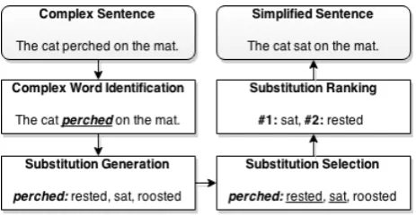
The goal of a Lexical Simplification (LS) system is to re-place the complex words in a text with simpler alternatives, without compromising its meaning or grammaticality. The LS task is often addressed as the series of steps in Figure 1, as introduced by (Devlin and Tait, 1998). Their work has inspired others to conceive new LS solutions for the aphasic (Carroll et al., 1998), dyslexic (Bott et al., 2012), illiterate (Watanabe et al., 2009), non-native English speakers (Paet-zold, 2013; Paetzold and Specia, 2013), children (Kajiwara et al., 2013) and others.
Figure 1: Lexical Simplification Pipeline
Although various LS systems can be found in the litera-ture, very little effort has been made to compare their per-formance. Apart from the work of (Shardlow, 2013) and (Specia et al., 2012), which provide brief benchmarkings of Complex Word Identification and Substitution Ranking, respectively, no other comparisons have been reported. To address this limitation, we present a systematic bench-marking of LS systems. We innovate by comparing the per-formance of not only systems in their entirety, but also of system components individually, such as Substitution Gen-eration, Selection and Ranking approaches. In addition, we introduce BenchLS, a new dataset for the task. In the fol-lowing Sections, we describe our dataset and present our experiments.
2.
BenchLS: A New Dataset
To create our dataset we combined two resources: the LexMTurk (Horn et al., 2014) and LSeval (De Belder and Moens, 2012) datasets. The instances in both datasets,929
in total, contain a sentence, a target complex word, and sev-eral candidate substitutions ranked according to their sim-plicity. The candidates in both datasets were suggested and ranked by English speakers from the U.S. To increase its reliability, we applied the following corrections over each instance of our dataset:
1. Spelling Filtering: We discard any misspelled can-didates using Norvig’s algorithm1. We trained our spelling model over the News Crawl2corpus.
2. Inflection Correction: We inflected all candidates to the tense of the target word using the Text Adorning module of LEXenstein (Paetzold and Specia, 2015; Burns, 2013).
The resulting dataset –BenchLS– contains929instances, with an average of7.37candidate substitutions per complex word. We use it in all our experiments, as described in what follows.
3.
Substitution Generation
Substitution Generation (SG) aims to produce candidate substitutions for complex words, which can be later ranked or filtered according to different criteria.
This step does not take into account the ambiguity of words, i.e. it generates candidate substitutions for a word in all or any of its possible meanings. The most frequently used SG solution consists in extracting synonyms from linguistic databases, such as WordNet (Devlin and Tait, 1998; Car-roll et al., 1999) or the UMLS database for medical content (Ong et al., 2007; Leroy et al., 2013). Recently, however,
1
http://norvig.com/spell-correct.html 2
new resources have been used, such as aligned complex-to-simple parallel corpora (Paetzold, 2013; Paetzold and Spe-cia, 2013; Horn et al., 2014) and word embedding models (Glavaˇs and ˇStajner, 2015; Paetzold and Specia, 2016).
3.1.
Systems
We re-implemented the following SG systems for evalua-tion:
• Devlin(Devlin and Tait, 1998): Extracts synonyms of complex words from WordNet 3.0 (Fellbaum, 1998).
• Biran(Biran et al., 2011): Creates the Cartesian prod-uct between Wikipedia and Simple Wikipedia by sim-ply pairing every word that appears in Wikipedia with every word in Simple Wikipedia. It then discards any pairs in which:
1. At least one of the words is a stop-word, numeral or punctuation.
2. The words share the same lemma.
3. The words are not registered as synonyms or hy-pernyms in WordNet.
• Yamamoto(Kajiwara et al., 2013): Given a complex word, it retrieves its definition from a dictionary, an-notates it using a POS tagger, and then extracts as can-didates any words that have the same POS tag as the complex word itself. This system queries the Mer-riam Dictionary3, and tags definitions with the Stan-ford Parser (Klein and Manning, 2003).
• Horn (Horn et al., 2014): Produces alignments for complex-to-simple parallel corpora, then extracts any
hcomplex→simpleipairs of aligned words in which:
1. The complex word is not a stop-word. 2. The POS tag of both words are the same.
3. Neither word is a proper noun.
To produce alignments, we use GIZA++ (Och and Ney, 2003). The words are then inflected to all their morphological forms using Morph Adorner (Burns, 2013). For this system, we use the parallel Wikipedia and Simple Wikipedia corpus (Horn et al., 2014) and the Stanford Parser.
• Glavas (Glavaˇs and ˇStajner, 2015): Produces candi-dates using a word embeddings model. They retrieve the10words for which the embeddings vector has the highest cosine similarity with that of the target com-plex word, except for its morphological variants. Their model uses200vector dimensions and is trained with the GloVe toolkit (Pennington et al., 2014). We train their model over a corpus of 7 billion words which combines combines the SubIMDB corpus (Paetzold, 2015), UMBC webbase4, News Crawl5, SUBTLEX (Brysbaert and New, 2009), Wikipedia and Simple Wikipedia (Kauchak, 2013).
3
http://www.merriam-webster.com/ 4
http://ebiquity.umbc.edu/resource/html/id/351 5
http://www.statmt.org/wmt11/translation-task.html
• Paetzold (Paetzold and Specia, 2016): Produces candidates using a context-aware word embeddings model. 10 candidates for each target word are re-trieved with a model trained using the word2vec toolkit (Mikolov et al., 2013) over the same corpus used for the Glavas generator, parsed with the Stan-ford Parser. Word vectors are trained using the Bag-of-Words (CBOW) architecture and1300vector dimen-sions.
3.2.
Datasets and Metrics
As a gold-standard, we use the candidate substitutions in BenchLS. The evaluation metrics are:
• Potential: Proportion of instances in which at least one of the candidates generated is in the gold-standard.
• Precision: Proportion of generated substitutions that are in the gold-standard.
• Recall: The proportion of gold-standard substitutions that are among the generated substitutions.
• F1: Harmonic mean between Precision & Recall.
3.3.
Results
Generator Pot. Prec. Rec. F1
Devlin 0.647 0.133 0.153 0.143
Biran 0.610 0.130 0.144 0.136
Yamamoto 0.360 0.032 0.087 0.047
Horn 0.569 0.235 0.131 0.168
Glavas 0.724 0.142 0.191 0.163
Paetzold 0.856 0.180 0.252 0.210
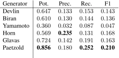
Table 1: SG benchmarking results
As illustrated in Table 1, the Paetzold generator outper-forms all others, including the supervised Horn generator, by a considerable margin in almost all metrics used, reveal-ing the potential of context-aware embeddreveal-ing models for SG. In order to further highlight the importance of using context-aware as opposed to traditional embedding models, we have trained a modified version of the Glavas generator. Instead of using the model specified in (Glavaˇs and ˇStajner, 2015), it uses a model trained with the same settings spec-ified for the context-aware model of the Paetzold genera-tor: the Bag-of-Words (CBOW) architecture of word2vec and1300 vector dimensions. The results depicted in Ta-ble 2 confirm that the difference in performance between the Glavas and Paetzold generator is indeed not due to model configuration, but rather the inherent differences be-tween traditional and context-aware embeddings.
Generator Pot. Prec. Rec. F1
Glavas (GloVe) 0.724 0.142 0.191 0.163
Glavas (CBOW) 0.708 0.142 0.193 0.164
Paetzold 0.856 0.180 0.252 0.210
Finally, the contrast between the high Precision and low Po-tential and Recall obtained by the Horn generator suggests that, while their technique is the most proficient in discard-ing spurious candidates, the alignments between Wikipedia and Simple Wikipedia offer considerably lower coverage than the linguistic regularities captured by word embedding models.
4.
Substitution Selection
Substitution Selection (SS) consists in deciding which of the generated substitutions fit the context of a target plex word. It aims to discard candidates which could com-promise the meaning and/or grammaticality of the text be-ing simplified.
Some previous work treat SS as a disambiguation task (Sed-ding and Kazakov, 2004; Nunes et al., 2013). They use sense labeling tools to determine the sense of a target word, and then discard any candidates which do not share said sense. Modern approaches have had noticeable success by using word co-occurrence models (Biran et al., 2011) and by joint modeling Substitution Selection and Ranking (Horn et al., 2014; Glavaˇs and ˇStajner, 2015).
4.1.
Systems
We re-implemented the following SS systems for evalua-tion:
• Lesk(Lesk, 1986): Uses the Lesk algorithm to deter-mine the sense of a target word, then selects only those candidates listed as synonyms in WordNet 3.0.
• Aluisio (Aluisio and Gasperin, 2010): Selects only candidates which can have the same POS tag as that of the target word. To learn which POS tags can be asso-ciated with each candidate, we first tag each sentence in the News Crawl corpus with the Stanford Parser and then collect word to POS tag counts. During Substitu-tion SelecSubstitu-tion, we discard any candidate substituSubstitu-tions that have not been tagged with the same tag as the tar-get complex word at least once in News Crawl.
• Belder(De Belder and Moens, 2010): Intersects the candidates generated for a target word with the words in a cluster in which the target word is included, as determined by a latent-variable language model. To replicate their approach, we learn2,000word clusters using the Brown clustering algorithm (Brown et al., 1992).
• Biran(Biran et al., 2011): Selects candidates using a word co-occurrence model. It first discards any candidates for which the cosine similarity between its co-occurrence vector and the co-occurrence vec-tor of the sentence in which the target was found is smaller than a threshold value t1. In order to avoid incoherent replacements, it then discards any candi-dates for which the cosine similarity between its com-mon co-occurrence vector with the target word and the co-occurrence vector of the sentence is larger than a threshold valuet2. We train the co-occurrence model over the same corpus used by the Paetzold generator.
We use the same values fort1 andt2 as in (Biran et al., 2011), which are0.1and0.01, respectively
• Paetzold(Paetzold and Specia, 2016): Treats Substi-tution Selection as a ranking problem, and employs a technique called Unsupervised Boundary Ranking to address it. During training, it first generates10 can-didate substitutions for the target word for each in-stance of BenchLS. It then exploits the assumption that words are irreplaceable, and creates training in-stances in unsupervised fashion by assigning label1
to the target word itself and0to all the remaining can-didates. After calculating feature values for each in-stance in the training set, it then learns a linear model through Stochastic Gradient Descent from it. During Substitution Selection, it ranks the candidates accord-ing to their distance from theboundarybetween pos-itive and negative instances, then keeps the 50% of candidates which are the furthest in the positive side. For features, we use the same ones from (Paetzold and Specia, 2016), which are:
1. Language model log-probabilities of the fol-lowing five n-grams: si−1c, csi+1, si−1csi+1, si−2si−1c and csi+1si+2, where c is a candi-date substitution, and i the position of the tar-get word in sentence s. We use a 5-gram lan-guage model trained over SubIMDB (Paetzold and Specia, 2016) with SRILM (Stolcke and oth-ers, 2002).
2. The word embeddings cosine similarity between the target complex word and a candidate. For this feature, we employ the same context-aware em-beddings model used by the Paetzold generator.
3. The conditional probability of a candidate given the POS tag of the target word. To calculate this feature, we learn the probability distribution P(c|pt), described in Equation 1, of all words in
the News Crawl corpus.
P(c|pt) = ceived tagpin the training corpus, andP the set of all POS tags.
We also include two baselines:
• First Sense: Selects only synonyms registered in the first sense of the target word in WordNet.
• No Selection: Selects all generated candidates.
4.2.
Datasets and Metrics
Selector Pot. Prec. Rec. F1 Lesk 0.337 0.053 0.075 0.062
Aluisio 0.916 0.098 0.398 0.157
Belder 0.297 0.188 0.057 0.088
Biran 0.478 0.068 0.185 0.099
Paetzold 0.851 0.166 0.284 0.209 First Sense 0.207 0.052 0.036 0.042
No Selection 0.940 0.062 0.438 0.109
Table 3: SS benchmarking results
4.3.
Results
As illustrated in Table 3, only the Aluisio and Paetzold selectors have managed to obtain higher F1 scores than not performing selection at all. While the Aluisio selector achieves better Recall, the Paetzold selector yields higher precision and F1. Although the Precision obtained by the Belder selector is the highest, it comes at noticeable losses in Potential and Recall.
5.
Substitution Ranking
Substitution Ranking (SR) is the task of ranking candidates by their simplicity. The goal is to replace the complex word by its simplest candidate substitute.
The most widely used SR strategy in the literature is metric-based ranking, in which candidates are ranked according to a manually crafted combination of features such as word frequency and length (Devlin and Tait, 1998; Carroll et al., 1998; Carroll et al., 1999; Biran et al., 2011; Bott and Sag-gion, 2011). Recently, however, more sophisticated super-vised approaches have been explored, such as SVM rankers (Horn et al., 2014) and Boundary Ranking (Paetzold and Specia, 2015).
5.1.
Systems
We re-implemented the following SR systems for evalua-tion:
• Devlin(Devlin and Tait, 1998): Ranks candidates ac-cording to their frequency in the Brown corpus (Fran-cis and Kucera, 1979).
• Biran (Biran et al., 2011): Employs the metric in Equation 2, in whichF(c, C)is the frequency of can-didatecin corpusC, andkckits length.
M(c) = F(c,Wikipedia)
F(c,Simple Wikipedia)× kck (2)
• Bott (Bott et al., 2012):Employs a sum of the metrics described in Equation 4 and 3.
scorewl(c) = p
kck −4 if kck ≥5 0 otherwise (3)
scoref req(c) =log(F(c,Simple Wikipedia)) (4)
• Yamamoto(Kajiwara et al., 2013): Ranks candidates according to the sum of various metrics, such as n-gram frequencies, word co-occurrence similarity and semantic distance to the target word.
• Horn(Horn et al., 2014): Uses Support Vector Ma-chines (Joachims, 2002) to learn a ranking model from data with several word and n-gram frequency features extracted from the Google 1T (Evert, 2010), Wikipedia and Simple Wikipedia corpora.
• Glavas(Glavaˇs and ˇStajner, 2015): Ranks candidates according to several features, such as n-gram frequen-cies and word vector similarity with the target word, and then re-ranks them according to their average rankings. The word embeddings model used is the same one used by the Glavas generator, and n-gram frequencies were extracted from the Google 1T cor-pus (Glavaˇs and ˇStajner, 2015).
• Paetzold(Paetzold and Specia, 2015): Uses a super-vised Boundary Ranking approach. It learns a rank-ing model from data usrank-ing a binary classification setup inferred from the ranking examples. This strategy is the same one used by the Paetzold selector, but instead of learning the ranking model from training data obtained in unsupervised fashion, it learns the model from manually annotated data.10 morphologi-cal, semantic and n-gram probability features selected through univariate feature selection are used. N-gram probabilities were extracted from a5-gram language model trained over the SubIMDB corpus (Paetzold and Specia, 2016).
5.2.
Datasets and Metrics
For this experiment, we randomly split the BenchLS dataset in training and test sets containing465and464instances, respectively. The metric used is TRank-at-n, which mea-sures the proportion of times in which a candidate with a gold-standard rankr≤nwas ranked first.
5.3.
Results
Ranker n=1 n=2 n=3
Devlin 0.457 0.630 0.665
Biran 0.472 0.617 0.707
Bott 0.519 0.657 0.704
Yamamoto 0.435 0.583 0.674
Horn 0.539 0.694 0.737
Glavas 0.526 0.674 0.746 Paetzold 0.547 0.701 0.743
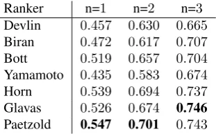
Table 4: SR benchmarking results
As illustrated in Table 4, although the Glavas ranker proved to be the most effective unsupervised system, the Paet-zold ranker has outperformed all others, including the SVM ranker of (Horn et al., 2014). These results highlight the ef-fectiveness of Boundary Ranking in capturing simplicity.
6.
Round-Trip Evaluation
6.1.
Systems
The systems included in our benchmarking are:
• Devlin(Devlin and Tait, 1998): Combines the Devlin SG and SR systems.
• Biran(Biran et al., 2011): Combines the Biran SG, SS and SR systems.
• Yamamoto(Kajiwara et al., 2013): Combines the Ya-mamoto SG and SR systems.
• Horn(Horn et al., 2014): Combines the Horn SG and SR systems.
• Glavas (Glavaˇs and ˇStajner, 2015): Combines the Glavas SG and SR systems.
• Paetzold(Paetzold and Specia, 2015): Combines the Paetzold SG, SS and SR systems.
6.2.
Datasets and Metrics
As a gold-standard, we use BenchLS. The Horn and Bound-ary ranker were trained on the LexMTurk dataset, which is used in (Horn et al., 2014), in order to avoid a bias on the results. The evaluation metrics used are the following:
• Precision: Ratio with which the highest ranking can-didate is either the target word itself or is in the gold-standard.
• Accuracy: Ratio with which the highest ranking can-didate is not the target word itself and is in the gold-standard.
• Changed Proportion: Ratio with which the highest ranking candidate is not the target word itself.
6.3.
Results
System Prec. Accu. Changed
Devlin 0.309 0.307 0.998
Biran 0.124 0.123 0.999
Yamamoto 0.044 0.041 0.997
Horn 0.546 0.341 0.795
Glavas 0.480 0.252 0.772
Paetzold 0.416 0.416 1.000
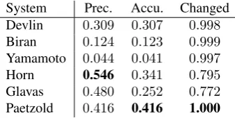
Table 5: Round-trip benchmarking results
As illustrated in Table 5, the Paetzold system has been shown the most accurate in practice, outperforming even simplifiers that rely on linguistic databases. The results also contrast with the ones reported in (Glavaˇs and ˇStajner, 2015), in which it was found no statistically significant dif-ference between the Horn and Glavas simplifiers: when evaluated over the BenchLS dataset, the supervised strategy of (Horn et al., 2014) is clearly more effective than that of (Glavaˇs and ˇStajner, 2015), offering an increase of almost
10% in Accuracy.
7.
Discussion and Conclusions
We have presented a benchmarking of Lexical Simplifica-tion systems based on BenchLS: a new dataset introduced for the task, which combines improved versions of two re-sources from previous work.
Through our benchmarks, we have discovered that exploit-ing the lexploit-inguistic regularities captured by context-aware word embedding models is a more reliable alternative to Substitution Generation than extracting complex-to-simple word correspondences from manually created parallel cor-pora. This finding is very important to the field because context-aware embedding models require only for large corpora of text and a POS tagger to be produced, and, un-like complex-to-simple parallel corpora, these resources are currently available for numerous languages.
Using these same resources, the Unsupervised Boundary Ranking approach of (Paetzold and Specia, 2016) offers an effective solution to Substitution Selection also. Because of its inherent difficulty and the ineffectiveness of early so-lutions, Substitution Selection has rarely been addressed in literature, which has consequently led modern simplifiers to simply ignore this step for the lack of a better alternative. We hope that our benchmarking results will inspire future authors to invest more time and resources in developing so-lutions to this step, which, as discussed in (Paetzold, 2015), can considerably increase the reliability of a simplifier.
In Substitution Ranking, supervised techniques seem to be the most effective. The strategies used by (Horn et al., 2014) and (Paetzold and Specia, 2015), which respectively employ an SVM and a Boundary Ranker, have obtained no-ticeably higher scores than the remaining unsupervised ap-proaches. Unlike rank averaging and metric-based strate-gies, supervised techniques are flexible, being able to au-tomatically learn which features should be used in mea-suring the simplicity of a candidate substitution. More importantly, this advantage comes at very little cost: the LexMTurk corpus, over which our supervised rankers were trained, contains only500instances.
In summary, we have found that the Paetzold simplifier is the most effective simplifier in practice. It generates can-didates substitutions using context-aware embedding mod-els, selects them through Unsupervised Boundary Ranking, and ranks them using a supervised Boundary Ranker. This approach has achieved the highest accuracy scores in our round-trip evaluation, meaning that it was the most profi-cient in correctly replacing complex words with simpler al-ternatives. When it comes to precision, however, the Horn simplifier was the one to achieve the highest score, mean-ing that it is the least likely to compromise the integrity of the sentence being simplified.
8.
Bibliographical References
Aluisio, S. and Gasperin, C., (2010). Proceedings of the NAACL 2010 Young Investigators Workshop on Com-putational Approaches to Languages of the Americas, chapter Fostering Digital Inclusion and Accessibility: The PorSimples project for Simplification of Portuguese Texts, pages 46–53. Association for Computational Lin-guistics.
Biran, O., Brody, S., and Elhadad, N. (2011). Putting it simply: a context-aware approach to lexical simplifica-tion. InProceedings of the 49th ACL, pages 496–501. Bott, S. and Saggion, H. (2011). An unsupervised
align-ment algorithm for text simplification corpus construc-tion. pages 20–26.
Bott, S., Rello, L., Drndarevic, B., and Saggion, H. (2012). Can spanish be simpler? lexsis: Lexical simplification for spanish. In Proceedings of 2012 COLING, pages 357–374.
Brown, P. F., deSouza, P. V., Mercer, R. L., Pietra, V. J. D., and Lai, J. C. (1992). Class-based n-gram models of nat-ural language.Computational Linguistics, 18:467–479. Brysbaert, M. and New, B. (2009). Moving beyond kuˇcera
and francis: A critical evaluation of current word fre-quency norms and the introduction of a new and im-proved word frequency measure for american english. Behavior research methods, 41:977–990.
Burns, P. R. (2013). MorphAdorner v2: A Java Library for the Morphological Adornment of English Language Texts.
Carroll, J., Minnen, G., Canning, Y., Devlin, S., and Tait, J. (1998). Practical simplification of english newspaper text to assist aphasic readers. InProceedings of AAAI-98 Workshop on Integrating Artificial Intelligence and Assistive Technology, pages 7–10.
Carroll, J., Minnen, G., Pearce, D., Canning, Y., Devlin, S., and Tait, J. (1999). Simplifying text for language-impaired readers. InProceedings of the 9th EACL, pages 269–270.
De Belder, J. and Moens, M.-F. (2010). Text simplification for children. InProceedings of the SIGIR Workshop on Accessible Search Systems, pages 19–26.
De Belder, J. and Moens, M.-F. (2012). A dataset for the evaluation of lexical simplification. In Computational Linguistics and Intelligent Text Processing, pages 426– 437. Springer.
Devlin, S. and Tait, J. (1998). The use of a psycholinguistic database in the simplification of text for aphasic readers. Linguistic Databases, pages 161–173.
Evert, S. (2010). Google web 1t 5-grams made easy (but not for the computer). InProceedings of the 2010 NAACL, pages 32–40.
Fellbaum, C. (1998). WordNet: An Electronic Lexical Database. Bradford Books.
Francis, W. N. and Kucera, H. (1979). Brown corpus man-ual.Brown University.
Glavaˇs, G. and ˇStajner, S. (2015). Simplifying lexical sim-plification: Do we need simplified corpora? In Proceed-ings of the 53rd ACL, page 63.
Horn, C., Manduca, C., and Kauchak, D. (2014). Learning
a Lexical Simplifier Using Wikipedia. InProceedings of the 52nd ACL, pages 458–463.
Joachims, T. (2002). Optimizing search engines using clickthrough data. InProceedings of the 8th ACM, pages 133–142.
Kajiwara, T., Matsumoto, H., and Yamamoto, K. (2013). Selecting Proper Lexical Paraphrase for Children. Pro-ceedings of the 25th Rocling, pages 59–73.
Kauchak, D. (2013). Improving text simplification lan-guage modeling using unsimplified text data. In Pro-ceedings of the 51st ACL, pages 1537–1546.
Klein, D. and Manning, C. D. (2003). Accurate unlexi-calized parsing. InProceedings of the 41st ACL, pages 423–430.
Leroy, G., Endicott, J. E., Kauchak, D., Mouradi, O., and Just, M. (2013). User evaluation of the effects of a text simplification algorithm using term familiarity on per-ception, understanding, learning, and information reten-tion. Journal of Medical Internet Research, 15.
Lesk, M. (1986). Automatic sense disambiguation using machine readable dictionaries: how to tell a pine cone from an ice cream cone. InProceedings of the 5th Con-ference on Systems Documentation, pages 24–26. Mikolov, T., Chen, K., Corrado, G., and Dean, J. (2013).
Efficient estimation of word representations in vector space.arXiv preprint arXiv:1301.3781.
Nunes, B. P., Kawase, R., Siehndel, P., Casanova, M. a., and Dietze, S. (2013). As Simple as It Gets - A Sentence Simplifier for Different Learning Levels and Contexts. pages 128–132.
Och, F. J. and Ney, H. (2003). A systematic comparison of various statistical alignment models. Comput. Linguist., 29(1):19–51, March.
Ong, E., Damay, J., Lojico, G., Lu, K., and Tarantan, D. (2007). Simplifying text in medical literature. volume 4, pages 37–47.
Paetzold, G. H. and Specia, L. (2013). Text simplification as tree transduction. InProceedings of the 9th STIL. Paetzold, G. H. and Specia, L. (2015). Lexenstein: A
framework for lexical simplification. InProceedings of The 53rd ACL.
Paetzold, G. H. and Specia, L. (2016). Unsupervised lex-ical simplification for non-native speakers. In Proceed-ings of The 30th AAAI.
Paetzold, G. H. (2013). Um Sistema de Simplificac¸˜ao Autom´atica de Textos escritos em Inglˆes por meio de Transduc¸ao de ´Arvores. Western Parana State Univer-sity.
Paetzold, G. H. (2015). Reliable lexical simplification for non-native speakers. InProceedings of the 2015 NAACL Student Research Workshop.
Pennington, J., Socher, R., and Manning, C. D. (2014). Glove: Global vectors for word representation. Proceed-ings of the 2014 EMNLP, pages 1532–1543.
Strouds-burg, PA, USA. Association for Computational Linguis-tics.
Shardlow, M. (2013). A comparison of techniques to auto-matically identify complex words. pages 103–109. Specia, L., Jauhar, S. K., and Mihalcea, R. (2012).
Semeval-2012 task 1: English lexical simplification. In Proceedings of the 1st SemEval, pages 347–355. Stolcke, A. et al. (2002). Srilm - an extensible language
modeling toolkit. InInterspeech.