R E S E A R C H
Open Access
Fractional difference co-array perspective
for wideband signal DOA estimation
Jian-Yan Liu
2,1, Yi-Long Lu
2, Yan-Mei Zhang
1and Wei-Jiang Wang
1*Abstract
In recent years, much attention has been focused on difference co-array perspective in DOA estimation field due to its ability to increase the degrees of freedom and to detect more sources than sensors. In this article, a fractional difference co-array perspective (FrDCA) is proposed by vectorizing structured second-order statistics matrices instead of conventional zero-lag covariance matrix. As a result, not only conventional virtual sensors but also the fractional ones can be utilized to further increase the degrees of freedom. In a sense, the proposed perspective can be viewed as an extended structured model to generate virtual sensors. Then, as a case study, four DOA estimation algorithms for wideband signal based on the FrDCA perspective are specifically presented. The fractional virtual sensors can be generated by dividing the wideband signal into many sub-band signals. Accordingly, the degree of freedom and the maximum number of resolvable sources are increased. The corresponding numerical simulation results validate the advantages and the effectiveness of the proposed perspective.
Keywords: Fractional difference co-array, Wideband signal DOA estimation, Enhancement of DOFs, Virtual sensor
1 Introduction
Direction of arrival (DOA) estimation is a critical problem in phased-array radar signal processing field [1]. Con-ventional DOA estimation methods (e.g., MUSIC [2] and ESPRIT [3]) were mainly based on the overdetermined uniform linear array (ULA) model (more sensors than sources). To detect more sources than sensors and max-imize the spatial resolution, some non-uniform linear arrays (NLAs) were introduced into radar society, dating back to minimum redundancy arrays (MRAs) [4] or mini-mum hole arrays (MHAs) [5]. Many important advantages were validated in works [6–8] by forming augmented covariance matrices. Recently, due to the fact that second-order statistics (SOS) allowed us to gain more degrees of freedom (DOFs), several virtual co-array concepts based on SOS were proposed. Originally, the virtual array con-cept was used in multi-input multi-output (MIMO) radar system [9] through an active sensing scenario. Specifi-cally, the MIMO radar could generate a group of sum co-arrays (SCA) that increase DOFs from O(N +M)
*Correspondence: [email protected]
1School of Information and Electronics, Beijing Institute of Technology, 5
South Zhongguancun Street, Haidian District, 100081 Beijing, People’s Republic of China
Full list of author information is available at the end of the article
to O(NM). A similar but not identical difference co-array (DCA) concept was proposed in [10], which could also generate virtual array and increase DOFs fromO(N) toO(N2)in a completely passive scenario by using a new NLA geometry called nested array. Following this notion, some new geometries were further developed such as co-prime array [11], generalized co-co-prime array [12], super nested array [13, 14], and dynamic array [15]. In [16, 17], the authors utilized multiple frequencies to fill the missing co-array elements, thereby enabling the co-prime array to effectively utilize all of the offered DOFs. In [18], the authors combined the DCA and the SCA and then pro-posed difference co-array of the sum co-array (DCSC), which offered a significant enhancement in the DOFs in active sensing scenario. In addition, a more general con-cept called compressive covariance sensing (CCS) was proposed in [19] by focusing on the reconstruction of the SOS matrix from sub-Nyquist samples.
The aforementioned DCA-based models were limited in narrowband signal case. Therefore, P. Pal, the founder of the DCA model, proposed an auto-focusing based method in [20] to extend the co-array concept into wide-band signal case. However, the subspace information of many sub-bands has not been fully utilized due to the auto-focusing technique, and the maximum number of
resolvable sources was limited by the number of consec-utive integral lags in the co-array. In this article, as an extension, the fractional difference co-array (FrDCA) per-spective is proposed by introducing two fractional factors, which can generate either fractional difference sensor position or conventional integral difference ones. Such an extension would bring some advantages for the wide-band signal DOA estimation: the sub-wide-bands with different center frequencies would be converted into a set of sig-nal received from the fractiosig-nal virtual sensors. Then, one could choose any element positions of interest to perform DOA estimation. As a result, the degree of freedom and the maximum number of resolvable sources are increased. The article is organized as follows. In Section 2, the FrDCA model is proposed. Section 3 provides the wide-band DOA estimation models by using FrDCA. Numer-ical simulation results are provided in Section 4. Then, Section 5 concludes this paper. Notations: we use lower-case bold characters to denote vectors (e.g. a), upper-case bold characters for matrices (e.g. A), and upper-case outline letters for set (e.g. A). For a matrix
A, the symbols A∗,AT, and AH denote the complex conjugation, transpose, and conjugate transpose respec-tively.diag{A}denotes a column vector consisting of the main diagonal elements of matrix A. diag{a} denotes a diagonal matrix that uses the elements of vectoraas its diagonal elements.vec{A}denotes vectorization operator. The symbol and⊗ denote the Khatri-Rao product and Kronecker product, respectively. |A|denotes the car-dinality of set A, which is a measure of the number of elements of the setA.
2 Fractional difference co-array
2.1 Array signal model
Consider a NLA with M sensors at locations L = {l1,l2,. . .,lM} in units of half a minimal wave-length (denoted asd0). Assume thatDfar-field sourcessk impinge to the array from directionsθk,k = 1, 2,· · ·,D. Choosing an assumed sensor located at the origin of coordinates as the reference, the received data of thepth sensor can be expressed as:
xp(t)=D k=1sk
t−lpk+np(t) (1) wherek = d0sin(θk)/c,np(t)is the uncorrelated addi-tive Gaussian white noise of thepth sensor.
Based on array output model (1), assume that one can obtain anM×Mgeneralized SOS matrixGXX, which can be a covariance matrix (CM) or some time-frequency SOS matrices, such as cyclic correlation matrix (CCM) [21], in different cases.
GXX=AL(μ1f,θ)AHL(μ2f,θ)+W (2)
where μ1 and μ2 are two fractional factors; W is the total effect of noise, interfere and cross terms;
andAL(f,θ)denotes the array manifold, which depends
upon three parameters: the array formulationL, the cen-ter frequencyf, and the impinging DOAsθ:1
AL(f,θ)=aL(f,θ1),aL(f,θ2),· · ·,aL(f,θD) responding to the direction ofθk. Here, it should be noted thatis aD×Ddiagonal matrix. The motivation behind this diagonal form will be soon made clearly.
Then, we would introduce a basic property of vector-ization operation that will be useful in the sequel. For a diagonal matrixB,
One can refer to Theorem 2 of [22] for detailed proof. Based on (4),Gxxcan be vectorized into (5):
y=vec{GXX}
. We will further analyze the termAˆ(f,θ)by choosing two elements (e.g.pth,qth):
One can get the following two conclusions from Eqs. (5)∼(7).
Firstly, for an array/co-array signal model, a scaled change in the center frequency can be equivalent to a same scaled change in the element positions. This concept is the basic transformation strategy to perform DOA estimation of wideband signal in Section 3.2.
Secondly, the left items of (7) can be viewed as an aug-mented manifold of a virtual array with sensors located at D,D= μ1L−μ2L. Compared toAˆ(f,θ),Aμ1L−μ2L(f,θ) only includes all the distinct rows of Aˆ(f,θ); therefore, one can obtainAμ1L−μ2L(f,θ) = ˆSAˆ(f,θ), whereSˆ is a
2.2 Fractional difference co-array perspective
According to the above data model, we then propose the perspective and definition of FrDCA.
Definition 1[Fractional difference co-array]:Let us
consider an array consisting of M sensors at positions A,A = {a1,a2, ...,aN}, and then, for two given fractional factors μ1 and μ2, the fractional difference co-array is defined as the array consisting of a set of sensors at posi-tionsD(μ1,μ2):
D(μ1,μ2)μ1A−μ2A
{ci,j=μ1ai−μ2aj,∀1≤i,j≤M} (8)
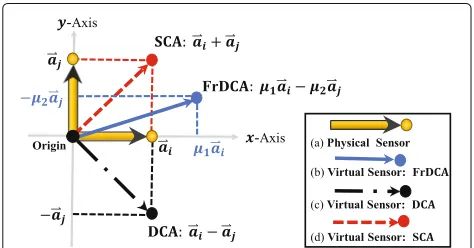
For any two physical sensors at locations{ai,aj}, Fig. 1 shows three kinds of co-arrays. Obviously, for any two physical sensors, their DCA and SCA are uniquely defined, while the FrDCA is dependent onμ1andμ2. As we know, any two numbersμ1andμ2can be expressed as μ1= α+βandμ2=α−β. Therefore, three situations are analyzed and compared according to differentαandβ:
1. α =0,β =0. For any pair-wise element positions,
ci,jandcj,i, one can obtain:
ci,j=β(ai+aj)+α(ai−aj) cj,i=β(ai+aj)−α(ai−aj)
(9)
Equation (9) indicates thatci,jandcj,iare
symmetrical with respect to theβ(ai+aj)-dot. Since
the(ai+aj)for different indexi,jis varied, the
FrDCA geometry is asymmetrical in this case. 2. α =0,β =0; The pair-wise element positions can be
expressed asci,j=α(ai−aj)= −cj,i, which indicates
that the FrDCA geometry is symmetrical with respect to the fixed zero-dot. Furthermore, ifα=1, thenci,j=(ai−aj)= −cj,i. The FrDCA becomes a
conventional DCA proposed in [10]. For a givenα, the corresponding FrDCA is aα-scaled conventional DCA,D(α,α)=αD(1, 1). Combing with (7), given a
Fig. 1The comparison of three kinds of co-arrays: the difference co-array, the sum co-array, and the fractional difference co-array
reference frequencyf and an operation frequencyfk,
then one can obtain aα-scaled FrDCAD(αk,αk), whereαk=fk/f. As a result, any desired virtual sensor position can be generated by choosing an appropriate operation frequencyfk. In a sense, such
FrDCA generated by multi-frequencies operation has been utilized in [16, 17] to fill the missing co-array elements, thereby enabling the co-prime array to effectively utilize all of the offered DOFs.
3. β =0,α=0; The pair-wise element positions can be expressed asci,j=β(ai+aj)=cj,i, which indicates
that the redundancy of any virtual sensor position is no less than two. Furthermore, ifβ=1, then
ci,j=(ai+aj)=cj,i. The FrDCA becomes a SCA.
For a givenβ, it is easy to find that the corresponding FrDCA is aβ-scaled SCA,D(β,−β)=βD(1,−1).
3 DOA estimation by using FrDCA
3.1 Review of narrowband signal based DCA model The conventional DCA perspective was proposed in [10]. Assume that the impinging source in (1) can be view as a narrowband uncorrelated model; hence, the array output can be expressed as
X(t)=AL(f,θ)s(t)+n(t) (10)
wheref denotes the center frequency ands(t)andn(t)are the source vector and noise vector, respectively. By collect-ingN snapshots, the covariance matrix can be estimated by (11)
RxxE{XXH}≈
1 N
N
t=1
X(t)X(t)H
=AL(f,θ)RssAHL(f,θ)+σ2IM
(11)
where IM denotes an M×M identity matrix, Rss the estimated covariance matrix of source signal, which is a diagonal matrix. It is entirely suited to the model in (2) withμ1=μ2=1.
y=vec{Rxx}
=A∗L(f,θ)AL(f,θ)p+σ2vec{IM}
=ADCA(f,θ)p+σ21M
(12)
where 1M = vec{IM},p = diag{Rss} and the corre-sponding DCA can be expressed as D(1, 1) = {li − lj, 1≤i,j≤M}.
3.2 Wideband signal-based FrDCA model
In practice, some wideband signal applications, such as the spread spectrum communication and ultrawideband radar system, have been increasing recently. DOA esti-mation for such a wideband signal is also required. For a wideband signal, the envelope is distinct at different sen-sors; therefore, the array outputs cannot be simply formed into a matrix form as (10). The received signal from each sensor can be divided intomindependent sub-bands with different center frequencies by performing discrete Fourier transform (DFT). Assume that their center fre-quencies are denoted as{f1,f2, ...fm}. Then, by choosing a center frequencyfcas a reference, theith frequency can be normalized asfi = αifc, whereαiis a fractional ratio. For a given array structureL, theith sub-band signal can be denoted as
Xi=AL(fi,θ)Si+Wi (13)
where i = 1, 2,· · ·,m; fi,Si, and Wi denote the center frequency, source vector, and noise vector of theith sub-band signal, respectively. Then, the covariance matrix can be formed by (14)
Rxx(fi)=AL(fi,θ)Rss(fi)AHL(fi,θ)+σni2IM
=AL(αifc,θ)Rss(fi)AHL(αifc,θ)+σni2IM
(14)
where Rss(fi) is a diagonal matrix under the assumption of uncorrelated sources for each frequency fi,Rss(fi) = diag δ2si,1 δsi2,1 · · · δsi2,D,δsi2,k is the power of kth source atith sub-band. All the signal power can be esti-mated by averaging the diagonal elements of Rss(fi) :
¯
Unlike the case of narrowband single frequency, Eq. (14) would be vectorized into (16) combing with an operation of signal power adjustment: is a ratio, which indicates the level of thekth signal power to the level of total received signal power (including noise power) in theith sub-band.
Based on the model in (16), the corresponding FrDCA can beDi(αi,αi). Due to the redundancy of the co-array,
|Di(αi,αi)| ≤ M(M−1), one can average the repeated
rows and reduce theM2dimensional model in (16) into a |Di|dimensional model in (17):
yDi(fi)=ADi(fc,θ)pi+γnieDi
behaves like an augmented array manifold containing a virtual array manifold matrixAˆDi(fc,θ); and a noise-related vectoreDi;pˆi =
pTi γniT behaves like an equivalent input signal, which is only dependent on the proportion of each signal power.
The reduced model in (17) is a complex valued signal model generated by averaging the element of covariance matrix. As we know, for the covariance matrix,Rxx(i,j)=
Rxx(j,i)∗. Therefore, if we let the elements of setDito be listed in an ascending order, one can separate the real and imaginary parts ofyDi(fi)by making use of the conjugate
symmetry of covariance matrix :
(yDi)=yDi+J|Di|yDi matrix. For the model (18), there are two important remarks.
Firstly, we focus on AˆDi. Based on the definition of Di(αi,αi) in (8), one can obtain that the elements in Di(αi,αi)are pair-wise,ci,j = −cj,i, which leads that the corresponding steering vectors are conjugate,aci,j = a∗cj,i. Therefore,AˆDi+J|Di|AˆDiis the real-valued matrix, while
ˆ
ADi−J|Di|AˆDiis the imaginary valued matrix.
Secondly, we focus on(yDi)and(yDi). The elements of these two real-valued vectors are symmetric charac-ter sequences, respectively. Therefore, one can construct a real-valued signal model as (19) by selecting the first|Di|+2 1 rows of(yDi)and the first|Di|−2 1rows of(yDi)
Based on this real-valued signal model in (20), the out-put signals z(fi) corresponding to different frequencies share the same spatial support. Therefore, without loss of generality, joint sparse recovery (joint CS) techniques can be applied for DOA estimation:
Z1=z(f1)T z(f2)T · · · z(fm)TT block diagonal matrix. (21) is a joint sparse DOA recon-struction model without considering signal properties.
If the ratio of each signal power can be independent of frequencyfi,pˆi = ¯p1,i=1, 2, ...,m, all the vectorized sig-nals in (16) can be directly stacked into a longer virtual signal in (22) and an augmented FrDCA in (23):
Z1=z(f1)T z(f2)T · · · z(fm)TT pling matrix and Z1 and p¯1 denotes input signal and output signal, respectively.
3.3 Sparse DOA recovery algorithm
After obtaining the array model in (21) and (22), DOA estimation can be performed mainly based on two methodologies: compressive sensing (CS) and subspace fitting (SSF).
Choosing the CS methodology, by dividing the region of interest into a finite gridθˆ, whereθˆ= { ˆθ1,θˆ2,· · ·,θQˆ }, one could establish an augmented array manifold ADi(fc,θ)ˆ and further build the corresponding over-complete dic-tionaries i(fc,θ)ˆ and i(fc,θ)ˆ . Equation (21) can be rewritten as (24)
Z1=1(fc,θ)ˆ p˜1(θ)ˆ ∈RL1×1 (24)
where1(fc,θ)ˆ ∈ RL1×m(Q+1) andp˜1(θ)ˆ ∈ Rm(Q+1)×1.
SinceQD, the signalpˆiis aDsparse vector in this set-ting. Then, the general objective function for this problem is (25) and denotes the error tolerance of noise dependence. Similarly, (22) also can be rewritten as (26)
Z1=1(fc,θ)ˆ p¯1(θ)ˆ ∈RL1×1 (26)
where1(fc,θ)ˆ ∈ RL1×(Q+1)andp¯1(θ)ˆ ∈ R(Q+1)×1. The general objective function for this problem is (27)
minp¯1(θ)ˆ 1
subject toZ1−1(fc,θ)ˆ p¯1(θ)ˆ 2≤
(27)
To solve this problem, LASSO [23] is an effective algo-rithm. The objective function can be expressed as
¯
whereηis the penalty parameter of data dependence. In the model (24) and (26),Z1 is influenced by noise power γn,i. In order to avoid estimating noise power, one can remove all the zero-lag entities. As a result, the noise vector eDi in (17) can be removed accord-ingly. This operation would reduce one dimension of the over-complete dictionaries and slightly decrease the computation complexity.
If choosing the SSF methodology, which requires a set of uniformly distributed sensors, one could select and construct a virtual ULAU,
U= {−Lu, −Lu+1, · · ·, Lu−1, Lu} (29)
Strictly speaking2, Ushould be a subset of D1 so that the corresponding virtual signalYu received by the ULA Ucan be exactly selected fromY1,
Yu=SuY1=AU(f,θ)p¯1∈C(2Lu+1)×1 (30) dimensional selection matrix. In this setting, (30) behaves like a fully coherent ULA signal model; therefore, MUSIC algorithm combined with a rank restoring method [24, 25] can be applied to obtain a spatial spectraP(θ)˜ ,
P(θ)˜ = 1
||aU(θ˜,f)HU n||2
(31)
whereUnis the eigenvector of noise space, which can be estimated by performing eigenvalue decomposition of the rank restored covariance matrix.
3.4 Related remarks
as an extended or generalized virtual co-array concept. This relationship is intuitively illustrated in Fig. 1. Then, by using FrDCA perspective, the virtual co-array can be extended into the wideband signal case. A wideband signal can be divided into several narrow sub-bands (with differ-ent cdiffer-enter frequencies ), which can be further transformed into a group of signals (with a fixed center frequency) received from a virtual array.
On the wideband co-array model: to solve the prob-lem of wideband signal DOA estimation, generally, the signal would be divided into many sub-bands with dif-ferent center frequencies. Therefore, how to combine such multi-frequency sub-bands is the central problem. The authors in [20] combined the signal subspaces at different frequencies into one joint subspace at the cho-sen frequency by introducing an auto-focusing matrix. Combing with the sparse array configuration, theoreti-cally, more wideband sources than physical sensors can be resolved. However, the subspace information of many sub-bands was not been fully utilized due to the auto-focusing technique, which just cast all the subspaces into a joint one with a desired center frequency. By using the proposed FrDCA concept, all the sub-bands can be fully utilized to generate virtual sensors and to increase the DOF capacity. Therefore, the proposed algorithm can resolve more wideband sources than sensors (even than the DCA-based uniformly virtual co-sensors). These advantages would be validated in the following simulation section.
On the sparse recovery model: in this paper, by uti-lizing the conjugated-symmetrical property of the virtual signal model, we establish a real-valued sparse recovery model. Therefore, compared to the prior proposed com-plex valued sparse recovery model in [17, 18, 20, 26], the computation complexity is reduced.
The author in [16, 17] proposed a multi-frequency co-prime array concept. This technique requires to actively transmit/receive some narrowband signals with different frequencies in different time slots, so that the covari-ance matrices of the received signals can exactly fill the missed holes in the co-array, as a result, the DOF capacity of co-array can be enhanced accordingly. In this active-like scheme, the center frequencies and time slots must be pre-planed before transmitting the certain waveforms. The proposed algorithm just requires to receive a wide-band signal, which behaves more like a passive scheme. As a result, no such pre-planed time slot is required and the center frequencies can be accordingly chosen/adjusted after receiving the wideband signal. In addition, the prior multi-frequency technique only make use of the posi-tion of integral virtual sensor. For the proposed tech-nique, all the positions including fractional ones can be directly presented and utilized. One can select any sen-sors of interest by adjusting a particular center frequency.
Therefore, the FrDCA concept provide a more flexible strategy.
How to properly select the center frequency fk? For a given physical arrayLand a wideband signal, whose fre-quency spectrum of interest can cover fromfmintofmax, one can uniquely determine D(1, 1) = L− L. Then, if one requires a sensor located atck, all the potential fac-torsαkare given byck ∈ αkD(1, 1),αk ∈ D(ck1,1). Take the corresponding center frequencyfk and the bandwidth of sub-bandk into consideration, the constrain condition can be expressed asfmin ≤αkf0±0.5k ≤fmax. In prac-tice, using the most adjacent sensor to fill this position is the best choice, which can result in the least frequency offset.
4 Numerical experiments
In this section, we conduct some numerical experiments by using MATLAB. To solve the (joint) CS problem, we use CVX toolbox, a package for specifying and solving convex programs [27, 28].
4.1 FrDCA-based MUSIC algorithm
In the first experiment, considering a NLA with sensors located atL = {0, 1, 4, 10, 12, 17}λ2 (where λis the minimal wavelength of signal) and assuming thatD Lin-ear Frequency Modulated (LFM) sources with 10-MHz bandwidth and 20-MHz center frequency uniformly distributed in space from −52◦ to 52◦, all the LFM sources have random initial phases and different initial frequencies in order to prevent coherence. Four thousand samples are collected at the sampling rate of 80 MHz for 50 μs. The SNR is 15 dB. The frequency spectrum of interest is from 15 to 25 MHz. Firstly, we focus on the conventional difference co-array D(1, 1) = L− L. The positions of the virtual sensors and the correspond-ing redundancy are illustrated in Fig. 2a. Obviously, its consecutive lags are from−13 to 13. There are holes at positions ±14 and ±15. The aforementioned analyses have pointed out that D(αk,αk) is theαk-scaled D(1, 1). Therefore, in order to fill the holes at positions ±14, there are many potential choices forαk, such as 1417,1416,1413, and so on. Combing all the holes into consideration, we divide the wideband signal into the following eight sub-bands with αk being {1416,1516,1616,1816,1916,2016,2216}. The corresponding center frequencies can be αkf0 , where f0 is the reference center frequency. All the selected center frequencies should be within the frequency spectrum of interest, 15 MHz ≤ αkf0 ≤ 25 MHz. Under this constraint, we can chose f0 = 18 MHz.
The corresponding center frequency fk =
a
b
Fig. 2The positions of virtual sensors.aThe conventional DCAD(1, 1)and the corresponding redundancy andbFrDCAD(αk,αk)for different sub-band signals, where the selected uniformly distributed sensorsUare marked with red face color
bandwidth of each sub-band should be much less than the center frequencyfk. Therefore, we chose the bandwidth as 0.6 MHz.
For DOA estimation based on MUSIC algorithm, we can select a set of consecutive and uniformly dis-tributed lags, as presented by the symbol with red face color in Fig. 2b. The virtual ULA can be U =
{−22,−21,· · ·, 21, 22}. Compared to the conventional DCA, the one-side aperture of virtual array is increased from 13 to 22. It validates that, by using the FrDCA con-cept, the wideband signal received from an array can be divided into a set of narrowband signal received from a larger aperture array with enhanced DOF capacity.
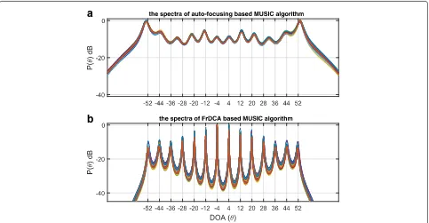
In the first experiment, consider nine uncorrelated LFM sources impinging to the array from the directionθ,θ =
{−52◦, −39◦, · · · , 39◦, 52◦}, and make a comparison with the auto-focusing based MUSIC algorithm in [20]. For auto-focusing-based MUSIC algorithm, in order to make fully use of all the virtual sensor, the correlation elements corresponding to the holes are assigned with zero. In this case, the virtual aperture can be increased to 17 other than 13. The MUSIC spectra of 30 indepen-dent trials for two kinds of algorithm are illustrated in Fig. 3. It shows that all the nine sources can be detected
by two algorithms. However, making a further compari-son between the peaks of the spectra, the peaks on the FrDCA-based MUSIC spectra are much sharper, which means that the estimated results are more accurate and precise.
In the second experiment, increase the number of sources to 14,θ = {−52◦, −46◦, · · · , 46◦, 52◦}. The MUSIC spectra of 30 independent trials are illustrated in Fig. 4. It shows that the auto-focusing-based MUSIC algorithm cannot work in such a multi-source condi-tion, while the FrDCA-based algorithm can clearly and correctly detect all the 14 sources.
4.2 FrDCA-based CS algorithm
In this section, we test the FrDCA-based CS algo-rithm. Compared to the MUSIC algorithm, it does not require the consecutive lags. Therefore, we chose αk and f0 as follows: f0 = 16 MHz, αk = {15.3
16 ,1616,1816,1916,2016,1621,2216,2316,2416,24.716 }. The other parame-ters are set as they are before. In this setting, a much larger virtual aperture is obtained.
a
b
Fig. 3The spectra of two algorithms:athe auto-focusing-based MUSIC andbthe FrDCA-based MUSIC by using a six-element NLA from an environment containing nine wideband signals
grid interval of ˆθ = 0.25◦and the penalty parameter of η=0.55 are used. The normalized spectra of 30 indepen-dent trials for two kinds of CS algorithms are illustrated in Fig. 5. By using CVX toolbox to solve the two models at the same platform, based on the run-time information
of CVX, the total CPU time for CS model in (28) is 0.51 s, while 7.34 s for joint CS model in (25). Then, a further comparison on the spectra shows that, generally, the two algorithms can resolve all the sources clearly and correctly with some sharp peaks. Specifically, the joint CS algorithm
a
b
a
b
Fig. 5The normalized spectra of two algorithms:athe FrDCA-based CS andbthe FrDCA-based joint CS by using a six-element NLA from an environment containing nine wideband signals
relatively outperforms the CS model because the former takes the signal power fluctuation into full consideration. There are some low-level background noise, as shown in the spectra of CS algorithm, which are mainly generated by the power approximation.
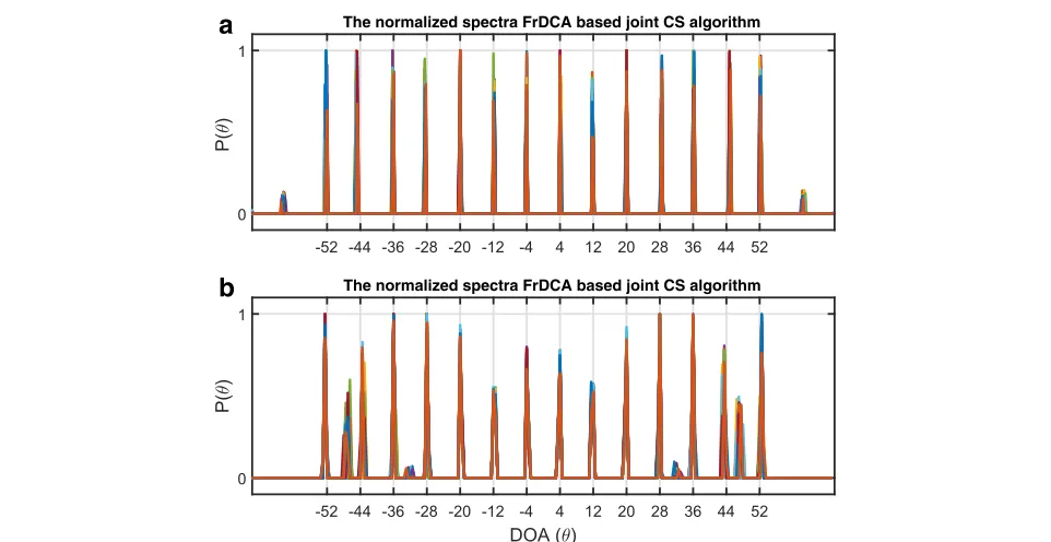
In the fourth experiment, increase the number of sources to 14. The normalized spectra of 30 independent trials are illustrated in Fig. 6. It shows that the per-formance of FrDCA-based joint CS algorithm is greatly reduced. Many false peaks are presented in the spectra
a
b
because the joint CS model does not possess enough DOF capacity to resolve so many sources. However, the CS algorithm can still maintain a good performance due to the increased DOF capacity.
4.3 RMSE
In this section, the performance of DOA estimation is compared via Monte Carlo trials. Hence, we define the average root-mean-square error (RMSE) of the estimated DOAs from 100 Monte Carlo trials as:
RMSE=
1
100D 100
n=1 D
k=1
(θk˜ (n)−θk)2 (32)
where θk(˜ n)is the estimation of θk for thenth trial. We compare how the SNR affects the DOA estimation.
The performances of four kinds of algorithms as a func-tion of the input SNR or the number of snapshots are quantified by the RMSE of 100 independent trials in the aforementioned two simulation conditions (D = 9, 14). The other parameters are set as they are before. The RMSEs corresponding to different SNR for four kinds of algorithms are illustrated in Figs. 7 and 8, respec-tively. It is observed that three kinds of FrDCA-based algorithms generally outperform the auto-focusing-based MUSIC algorithm in all the conditions. The FrDCA-based joint CS algorithm achieves the best performance when the number of impinging source is 9, while its perfor-mance is reduced when the number of impinging source is increased to 14. The FrDCA-based MUSIC and CS algorithm is efficient and robust for the multi-source con-dition, especially when SNR ≥ 0 dB. However, their performances are greatly reduced when SNR < 0 dB.
-10 -5 0 5 10 15 20 25
SNR (dB) 0
0.2 0.4 0.6 0.8
RMSE (Deg)
FrDCA based CS FrDCA based Joint CS FrDCA based MUSIC auto-focusing based MUSIC
Fig. 7The comparison of RMSEs corresponding to different SNR for four kinds of algorithms by using six-element array from an environment containing nine wideband signals
-10 -5 0 5 10 15 20 25
SNR (dB) 0
0.2 0.4 0.6 0.8
RMSE (Deg)
FrDCA based CS FrDCA based Joint CS FrDCA based MUSIC auto-focusing based MUSIC
Fig. 8The comparison of RMSEs corresponding to different SNR for four kinds of algorithms by using six-element array from an environment containing 14 wideband signals
The RMSEs corresponding to different number of snap-shots are illustrated in Fig. 9. It is observed that the proposed FrDCA-based algorithms have already estab-lished a clear superiority. As the number of snapshots decreased, the signal power ( variance matrix ) estimation error are accordantly increased. Such estimation errors, which could be viewed as power fluctuation, would be spread in the FrDCA-based CS/MUSIC model. Therefore, their performance are greatly reduced in small number of snapshots compared to the joint CS algorithm.
4.4 The case of power fluctuation
In this section, we focus on the case of power fluctua-tion; assume that 9 LFM sources with 2-MHz bandwidth
2400 2800 3200 3600 4000 4400
The Number of Snapshots 0
0.2 0.4 0.6
RMSE (Deg)
FrDCA based CS FrDCA based Joint CS FrDCA based MUSIC auto-focusing based MUSIC
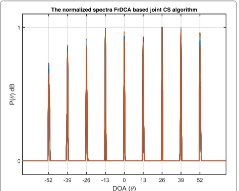
andfckMHz center frequency are uniformly distributed in space from−52◦to 52◦, wherefck = {16, 17, 18,· · ·, 24}. In this setting, the signal power is significantly fluctuant and the FrDAC-based CS and MUSIC algorithms fail to work. We test the FrDCA-based joint CS algorithms by dividing the wideband signal into nine sub-bands based on the following parameter:fk = {16, 17,· · ·, 24}MHz,f0= 20 MHz, the bandwidth of all the sub-bands is 1 MHz. The normalized spectra of 30 independent trials are illustrated in Fig. 10. It shows that the joint CS algorithm can success-fully resolve all sources in such a case of power fluctuation. The sharp peaks in the spectra indicate that the effective-ness of the algorithm and the measurement accuracy and precision are favorable.
5 Conclusions
Following the DCA perspective, we propose a FrDCA perspective by vectorizing structured SOS matrices. In a sense, it can be viewed as an extended structured model to generate virtual sensors including not only the conven-tional virtual sensors but also fracconven-tional ones. In practice, three DOA estimation algorithms for wideband signal based on proposed FrDCA are specifically presented. A wideband signal can be divided into several sub-band signals with different center frequencies. Then, by using FrDCA perspective, these sub-band signals can be fur-ther transformed into a group of virtual array signal with a fixed reference center frequency. In addition, by using the wideband signal to increase DOF capacity, more wide-band sources than sensors (even more than virtual co-sensors) can be resolved. In the end, the corresponding numerical simulation results validate the advantages and
Fig. 10The spectra of the FrDCA-based joint CS algorithm by using a six-element NLA from environment containing nine wideband signals of power fluctuation
the effectiveness of the proposed perspective through the performance comparisons with the existing algorithm.
Endnotes
1In the sequel, by analogy,A
Di(μ1f,θ)denotes the array manifold with the center frequency being μ1f and the array formulation beingDi.
2To fully make use all the virtual sensors, a small
num-ber of correlation elements corresponding to the holes can be assigned with zero. In this setting,U D1 and the performance may be marginally improved.
Acknowledgements
Mr. Jianyan LIU gratefully acknowledges financial support from China Scholarship Council (CSC NO. 201506030035). The authors greatly appreciate the constructive and insightful comments from the associate editor and reviewers that enabled us to improve the manuscript considerably.
Competing interests
The authors declare that they have no competing interests.
Author details
1School of Information and Electronics, Beijing Institute of Technology, 5
South Zhongguancun Street, Haidian District, 100081 Beijing, People’s Republic of China.2School of Electrical and Electronic Engineering, Nanyang Technological University, 50 Nanyang Avenue, Singapore, 639798, Singapore.
Received: 7 September 2016 Accepted: 18 November 2016
References
1. SH Talisa, KW O’Haver, TM Comberiate, MD Sharp, OF Somerlock, Benefits of digital phased array radars. Proc. IEEE.104(3), 530–543 (2016) 2. RO Schmidt, Multiple emitter location and signal parameter estimation.
IEEE Trans. Antennas Propag.34(3), 276–280 (1986)
3. R Roy, T Kailath, Esprit-estimation of signal parameters via rotational invariance techniques. IEEE Trans. Acoust. Speech Signal Process.37(7), 984–995 (1989)
4. A Moffet, Minimum-redundancy linear arrays. IEEE Trans. Antennas Propag.16(2), 172–175 (1968)
5. E Vertatschitsch, S Haykin, Nonredundant arrays. Proc. IEEE.74(1), 217–217 (1986)
6. SU Pillai, Y Bar-Ness, F Haber, A new approach to array geometry for improved spatial spectrum estimation. Proc. IEEE.73(10), 1522–1524 (1985)
7. SU Pillai, F Haber, Statistical analysis of a high resolution spatial spectrum estimator utilizing an augmented covariance matrix. IEEE Trans. Acoust. Speech Signal Process.35(11), 1517–1523 (1987)
8. YI Abramovich, NK Spencer, AY Gorokhov, Detection-estimation of more uncorrelated Gaussian sources than sensors in nonuniform linear antenna arrays .I. fully augmentable arrays. IEEE Trans. Signal Process.49(5), 959–971 (2001)
9. J Li, P Stoica,MIMO Radar Signal Processing. (John Wiley and Sons Press, USA, 2009), pp. 365–410
10. P Pal, PP Vaidyanathan, Nested arrays: a novel approach to array processing with enhanced degrees of freedom. IEEE Trans. Signal Process.
58(8), 4167–4181 (2010)
11. PP Vaidyanathan, P Pal, Sparse sensing with co-prime samplers and arrays. IEEE Trans. Signal Process.59(2), 573–586 (2011)
12. S Qin, YD Zhang, MG Amin, Generalized coprime array configurations for direction-of-arrival estimation. IEEE Trans. Signal Process.63(6), 1377–1390 (2015)
13. CL Liu, PP Vaidyanathan, Super nested arrays: linear sparse arrays with reduced mutual coupling-part i: Fundamentals. IEEE Trans. Signal Process.
14. CL Liu, PP Vaidyanathan, Super nested arrays: linear sparse arrays with reduced mutual coupling-part ii: High-order extensions. IEEE Trans. Signal Process.64(16), 4203–4217 (2016)
15. DD Ariananda, G Leus, Direction of arrival estimation for more correlated sources than active sensors. Signal Process.93(12), 3435–3448 (2013) 16. E BouDaher, Y Jia, F Ahmad, MG Amin, Multi-frequency co-prime arrays
for high-resolution direction-of-arrival estimation. IEEE Trans. Signal Process.63(14), 3797–3808 (2015)
17. E BouDaher, F Ahmad, MG Amin, Sparse reconstruction for direction-of-arrival estimation using multi-frequency co-prime arrays. EURASIP J. Adv. Signal Process.2014(1), 1–11 (2014)
18. E BouDaher, F Ahmad, MG Amin, Sparsity-based direction finding of coherent and uncorrelated targets using active nonuniform arrays. IEEE Signal Process. Lett.22(10), 1628–1632 (2015)
19. D Romero, DD Ariananda, Z Tian, G Leus, Compressive covariance sensing: structure-based compressive sensing beyond sparsity. IEEE Signal Process. Mag.33(1), 78–93 (2016)
20. P Pal, PP Vaidyanathan, inSignals, Systems and Computers, 2009 Conference Record of the Forty-Third Asilomar Conference on. A novel autofocusing approach for estimating directions-of-arrival of wideband signals (IEEE, Pacific Grove, 2009), pp. 1663–1667
21. G Gelli, L Izzo, Minimum-redundancy linear arrays for
cyclostationarity-based source location. IEEE Trans. Signal Process.45(10), 2605–2608 (1997)
22. MJ R, N Heinz,Matrix Differential Calculus with Applications in Statistics and Econometrics. (John Wiley and Sons Press, USA, 2007), pp. 31–35 23. R Tibshirani, Regression shrinkage and selection via the lasso. J. Roy.
Statist. Soc. Ser. B Methodol.58(1), 267–288 (1996)
24. T-J Shan, M Wax, T Kailath, On spatial smoothing for direction-of-arrival estimation of coherent signals. IEEE Trans. Acoust. Speech Signal Process.
33(4), 806–811 (1985)
25. C-L Liu, PP Vaidyanathan, Remarks on the spatial smoothing step in coarray music. IEEE Signal Process. Lett.22(9), 1438–1442 (2015) 26. Q Shen, W Liu, W Cui, S Wu, YD Zhang, MG Amin, Low-complexity
direction-of-arrival estimation based on wideband co-prime arrays. IEEE/ACM Trans. Audio Speech Lang. Process.23(9), 1445–1456 (2015) 27. M Grant, S Boyd, CVX: Matlab Software for Disciplined Convex
Programming, version 2.1 (2014). http://cvxr.com/cvx. Accessed 19 July 2016
28. M Grant, S Boyd, inRecent Advances in Learning and Control. Lecture Notes in Control and Information Sciences, ed. by V Blondel, S Boyd, and H Kimura. Graph implementations for nonsmooth convex programs (Springer London, London, 2008), pp. 95–110. http://stanford.edu/~ boyd/graph_dcp.html
Submit your manuscript to a
journal and benefi t from:
7Convenient online submission 7Rigorous peer review
7Immediate publication on acceptance 7Open access: articles freely available online 7High visibility within the fi eld
7Retaining the copyright to your article