R E S E A R C H
Open Access
Fast algorithm for designing
periodic/aperiodic sequences with good
correlation and stopband properties
Liang Tang
*, Yongfeng Zhu and Qiang Fu
Abstract
Periodic/aperiodic sequences with low autocorrelation sidelobes are widely used in many fields, such as communication and radar systems. Besides the correlation property, the frequency stopband property is often considered in the sequence design when the systems work in a crowded electromagnetic environment. In this paper, we aim at designing periodic/aperiodic sequences with low autocorrelation sidelobes and arbitrary frequency stopbands, and propose an efficient algorithm named FFT (fast Fourier transform)-based conjugate gradient
algorithm. To calculate the step size efficiently, a method based on Taylor series expansion is developed. By changing the number of FFT points, the proposed algorithm can be easily used to generate periodic/aperiodic sequences. Since the gradient and step size can be implemented by FFT operations and Hadamard product, the whole algorithm is computationally efficient and can be used to design very long sequences. Numerical experiments show that the proposed algorithm has better performance than the state-of-the-art algorithms in terms of the running time.
Keywords: Autocorrelation, Integrated sidelobe level, Stopband property, Gradient, Periodic/aperiodic sequence design
1 Introduction
Sequences with low periodic or aperiodic autocorrela-tion sidelobes have been studied for a long time since the 1950s. The applications of such sequences cover both mil-itary field and civil field, such as the pulse compression radar and wireless communication [1,2]. In pulse com-pression radar, the output of the pulse comcom-pression can be regarded as the convolution of each scattering point and the waveform’s autocorrelation. As the traditional wave-forms (e.g., linear frequency modulation (LFM) signal) suffer high range sidelobes, the detection performance and imaging quality of radar systems are limited. Thus, sequences with low autocorrelation sidelobes are applied to suppress the sidelobe jamming from the adjacent strong scattering points and thus improve the detection perfor-mance of weak target [3]. Moreover, sequences with low autocorrelation sidelobes have many advantages in the code division multiple access (CDMA) systems [4], for
*Correspondence:[email protected]
1National University of Defense Technology, Deya Road, Changsha, China
instance, reducing the influence of the multipath effect and improving the synchronization precision.
Owing to the extensive application and great practical value of the sequences with low autocorrelation sidelobes, many scholars have shown a great interest in generating such sequences. The related studies can be classified into two categories. The first category is the design of binary sequences by using the search methodologies, such as exhaustive search method [5] and evolutionary algorithm [6]. And the second category is the design of polyphase sequences [7–13]. In recent years, with the development of the optimization theory, the problem of designing polyphase sequences with low autocorrelation sidelobes has been a research hotspot. Stochastic optimization algo-rithms [7, 8] were applied to design such sequences at the early stage. However, because of the high computa-tional burden, these algorithms are impractical and unable to design sequences with large length. In order to fix this problem more efficiently, algorithms named CAN (cyclic algorithm new) and Accelerated-MISL (acceler-ated monotonic minimizer for integr(acceler-ated sidelobe level) which were both based on fast Fourier transform (FFT)
were proposed in [9,10]. In [9], the CAN algorithm was proposed to design unimodular sequences of large length by minimizing a criterion which is “almost equivalent” to the integrated sidelobe level (ISL) metric. Different from the CAN algorithm, the Accelerated-MISL algo-rithm [10] was deduced via majorization-minimization (MM) method. Since the Accelerated-MISL algorithm is based on an acceleration scheme which can greatly reduce the iteration number, it outperforms the CAN algorithm on both the merit factor (MF) and the computational efficiency. Besides, there are some literatures on design-ing sequences with zero correlation zone [11–13] or low periodic autocorrelation [14].
Apart from the correlation property, the stopband prop-erty (which means suppressing several frequency bands) is usually considered in sequence design for suppressing narrowband interferences or avoiding the certain fre-quency bands that reserved for some applications, such as navigation and military communications [15–19]. Since the discontinuous frequency of the transmit waveform leads to high autocorrelation sidelobes, the correlation and stopband properties are both considered. At the early stage, the cyclic algorithms named SCAN (stopband CAN) and WeSCAN (weighted SCAN) were proposed in [20] to design sequences with good correlation and stopband properties. But since the WeSCAN requires
N FFT operations and the eigenvalue decomposition at each iteration, its convergence speed is slow. Afterwards, the improved cyclic algorithms named SDCA (steepest descent-based cyclic algorithm) [21] and MMSE-WISL [22] are proposed for sparse frequency waveform design on the basis of the CAN and WeCAN (weighted CAN) algorithms [9]. However, like the WeSCAN algorithm, these two improved algorithms are also time-consuming and not suitable for long waveform design [22]. In recent years, some efficient algorithms, such as the majorization-minimization (MM) method [10], gradient-based algo-rithms [23, 24], Lagrange programming neural network (LPNN) [25], alternating projection [26], and alternating direction method of multipliers (ADMM) [27], have also been applied to unimodular sequence design with stop-band property, where LPNN and ADMM can be applied to generate both the periodic and aperiodic waveforms. It is worth noting that the sidelobe suppression means flat-ting the sequence spectrum. Thus, the suppression of fre-quency stopbands seems more difficult than the sidelobe suppression, which means that suppressing the stopbands increases more complexity.
In this paper, we consider the problem of designing periodic/aperiodic sequences with low autocorrelation sidelobes and arbitrary frequency stopbands. By using the relationship between the autocorrelation function and power spectrum density (PSD), the problem is formu-lated as an unconstrained minimization problem with
respect to the sequence phase in frequency domain. To solve this problem, an efficient algorithm named FFT-based conjugate gradient algorithm (which we call FCGA) is proposed. Unlike the traditional gradient algo-rithm, the searching step size of the FCGA which is hard to calculate directly is deduced via the Tay-lor series expansion. As the gradient and step size of the FCGA can be implemented by FFT operations and Hadamard product, the algorithm is efficient and can design sequences with large length. Moreover, by select-ing the number of the FFT points, the proposed algo-rithm can be easily applied to design periodic or aperiodic sequences.
The remaining sections of the paper are organized as follows. In Section2, the sequence design problem that incorporates both the correlation and stopband properties is formulated. In Section 3, the phase gradient and step size are derived, and then, a modified descent direction is given to guarantee the monotonicity of the FCGA. To show the effectiveness of the proposed algorithm, several numerical experiments are presented in Section4. Finally, Section5gives the conclusion.
Notation: Boldface upper case letters denote matrices
while boldface lower case letters denote column vectors. (·)∗,(·)T, and(·)H denote the complex conjugate, trans-pose, and conjugate transtrans-pose, respectively. · denotes the Euclidean norm of vectors.◦denotes the Hadamard product.X(m,n)denotes the (mth,nth) element of matrix X. Re(·) and Im(·) denote the real and imaginary part, respectively. Diag(x)is a diagonal matrix formed withx. FN(·),FN−1(·) denote theN−point FFT and inverse FFT (IFFT) operations, respectively.
2 Problem formulation
As mentioned in Section1, this paper focuses on the prob-lem of designing sequences with good correlation and fre-quency stopband properties. That is to say, the sequences should satisfy two conditions: one is low autocorrelation sidelobes (here we minimize the power of the sidelobes, i.e., ISL metric); the other one is low stopband power. In the following, two criterions are established to measure the autocorrelation and the stopband power, and then, we formulate the design problem as an unconstrained minimization problem.
2.1 Correlation property
Let{xn}Nn=−01denote the complex sequence to be designed.
The vector form of the sequence can be expressed as
x=[x0, ...,xN−1]T. (1)
˜
Then, the corresponding integrated sidelobe levels (ISLs) which express the goodness of the periodic and aperiodic correlation properties are given by
Iper=
denote the periodic and aperiodic autocorrelation vec-tors, respectively. Then,IperandIapercan be written more compact as
N× ˜Ndiscrete Fourier transform (DFT) matrix with the following expression
FN˜ (m,n)=e −j2mnπ
˜
N , 0≤m,n<N˜. (6)
Then, the N˜ × ˜N inverse discrete Fourier transform (IDFT) matrix isFH˜
N/N˜. It is well known that the auto-correlation function is the inverse Fourier transform of the power spectrum density (PSD); thus, we have the following relationship [13, 14]:
r1=FN−1(p1)= tively. By substituting (7) into (5), the frequency domain expressions ofIperandIaperare given by
Iper=
Generally, the problem of designing periodic/aperiodic sequences with low autocorrelation sidelobes can be regarded as a minimization problem of the peri-odic/aperiodic ISL metrics. From (8), it is easy to see that the metrics of the periodic and aperiodic autocorrela-tions have the same form. Thus, by ignoring the constant terms in (8), the periodic/aperiodic ISL metrics can be equivalent to the following unified criterion:
JACF= criterion for the aperiodic autocorrelation.
2.2 Stopband property
In crowded electromagnetic environment, the signal spec-trum is often polluted by the interference or the signals from other users. Thus, designing sequences with fre-quency stopbands is sometimes quite necessary. Without loss of generality, we consider the normalized frequencies here.
Assume the set of frequency stopbands ⊂ [0, 1] can be written as number of the stopbands. Considering theN˜−point FFT operations, the corresponding point set of the stopband set can be expressed as
1=
where· ,·are the floor and ceiling operations. There-fore, the suppression of the stopband setis equivalent to minimizing the PSD in1, i.e.,p(k),k∈1. Let us define
the frequency weight vector as
wf =
As the PSD is nonnegative, the criterion for the stop-band property can be constructed as the square of the Euclidean norm of the weighted PSD:
JPSD=wf ◦p2=pHDiag wf
p. (13)
2.3 The minimization problem
In order to suppress the autocorrelation sidelobes and the stopband power, both JACF andJPSD should be min-imized. Thus, the design problem can be regarded as a bi-objective optimization (or Pareto optimization) prob-lem. However, since the frequency stopband leads to high sidelobes, it is impossible to find a solution that minimizes bothJACFandJPSD. To make a compromise between cor-relation sidelobes and frequency stopbands, here we apply the scalarization procedure, i.e., turning the bi-objective optimization problem into a single-objective optimiza-tion problem. After scalarizing the problem, the single objective function that incorporates (9) and (13) can be expressed as
JT =λJPSD+(1−λ)JACF
=λpHDiag wf
p+ 1−λ 2N˜ p
Hp
=pHDiag(w)p.
(14)
whereλ ∈ [0, 1] is a weight coefficient by which we can balance the relative weight between JACF and JPSD, and
w=λwf +12−N˜λ.
Definingf = f0, ...,fN˜−1
T
as theN˜−point DFT ofx, and
ap=
1,ejωp, ...,ejωp(N−1)
T
,ωp= 2π ˜
N p,p=0, ...,N˜ −1,
(15)
then one can get
f=aH0x, ...,aNH˜−1xT.
p=f∗◦f=
xHa0aH0x, ...,xHaN˜−1aHN˜−1x
T
.
(16)
By substituting (16) into (14), the objective functionJT can be reformulated as
JT =
˜ N−1
p=0
wp
xHapaHpx
2
, (17)
wherewp = λw¯p+ 12−N˜λ is thepth element of the weight vectorw.
In general, the transmitter components such as power amplifier have a maximum amplitude clip [2]. To max-imize the transmitter power, it is desired for sequence amplitude to reach this amplitude clip, which means that the sequence should be unimodular. Therefore, consider-ing the unimodular constraint, the problem of interest can be written as
min JT = ˜ N−1
p=0
wp
xHapaHpx
2
s.t. |xn| =1, n=0, ...,N−1.
(18)
From (18), we can see that the unimodular constraint is the constraint related to the sequence amplitude. Thus, the minimization problem can be solved by optimizing the sequence phase. Let
φ=[φ0, ...,φN−1]T (19)
denote the phase vector of the sequencex, then we have
x=ejφ0, ...,ejφN−1T. (20)
Thus, the problem (18) can be seen as an unconstrained minimization problem onφ:
min JT(φ)= ˜ N−1
p=0
wp
xHapaHpx
2
. (21)
3 The FCGA algorithm
A good property of the Accelerated-MISL algorithm in [10] is the monotone decreasing property. But this algo-rithm minimizes the majorization function rather than the original function. To minimize the objective function (21) directly and guarantee the monotonically decreasing property of the algorithm, the conjugate gradient algo-rithm (CGA) is applied here. In this section, we first deduce the gradient and the step size, which are two important parts of the CGA, and then summarize the FCGA algorithm.
3.1 Phase gradient
To deduce the phase gradient∇φJT, we first work out the derivative of the functionJT(φ)with respect to the phase φi,i=0, ...,N−1:
∂JT ∂φi =2
˜ N−1
p=0
wp
xHapaHpx
∂xHa
paHpx
∂φi . (22)
Let
Ap=apaHp, Ap(m+1,n+1)=apmn, 0≤m,n≤N−1. (23)
Then, the gradient∇φJTcan be written as
∇φJT =2 ˜ N−1
p=0
wp xHApx
∇φ xHApx
. (24)
In the following, we derive the explicit expression of ∇φ xHApx
xHApx= derivative (26) can be rewritten as
∂xHApx
According to (24) and (28), the explicit expression of phase gradient is given by (see the Appendix1)
∇φJT =4N˜Re −jx∗◦y1:N
3.2 Step size calculation via Taylor series expansion
The traditional methods for obtaining the step size are the linear search methods. As the linear search methods cost much iteration and computation, the best way to obtain the step size is direct calculation. In this subsection, we adopt the Taylor series expansion to deduce the step size.
Assume the present iteration point isxk, and the
corre-sponding iteration direction isdk=
dk0, ...,dNk−1T. Then, the next iteration point can be expressed as
φk+1=φk+μdk,xk+1=xk◦
whereμis the step size. Essentially, the linear search prob-lem is a minimization probprob-lem with respect to μwhich can be expressed as follows:
min
then the derivative of JT(μ) with respect to μ can be written as of xk anddk. By using the Taylor series expansion and then keeping the first three terms, the exponential term
By substituting (39) into (34), the derivative in (34) can be written more compactly as
∂JT(μ) ∂μ
= −4wT
fk2−2μt2−μ2t1
◦(t2+μt1)
= −4 aμ3+bμ2+cμ+d,
(41)
where
a= −wT(t1◦t1),
b= −3wT(t1◦t2),
c= −2wT(t2◦t2)+wT
fk2◦t1
,
d=wT
fk2◦t2
.
(42)
Let∂JT(μ)/∂μ=0, then we have
aμ3+bμ2+cμ+d=0. (43)
It is well known that there is at least a real root in the roots of a cubic equation with real coefficients. Thus, the approximate step size can be calculated directly by solving (43). Since the searching direction is descendant, problem (32) has at least one minimum point greater than 0. Then, we can choose the positive root of (43) which is closest to zero as the step size.
3.3 Algorithm summary
After deducing the phase gradient and the step size, it is easy to solve the unconstrained problem (21) by using the conjugate gradient algorithm (CGA). In order to calculate the search direction effectively, here we apply the classical Polak-Ribiere-Polyak-CGA (PRP-CGA) whose direction can be calculated according to the gradient. The searching direction of the PRP-CGA can be expressed as
dk+1= −gk+1+ g
k+1−gkTgk+1
gk2 d
k, (44)
where gk and dk are the gradient and searching direc-tion of thekth iteration, respectively. Since the step size is an approximate value, gk+1Tdk may not be zero. Thus, dk+1may not be descendant, i.e.,
gk+1Tdk+1
= −gk+12+ g
k+1−gkTgk+1
gk2
gk+1Tdk <0
(45)
is not always satisfied. For guaranteeing that the searching direction is descendant, we apply the following modified direction:
˜
dk+1= −gk+1+ g
k+1−gkTgk+1
gk2 d
k,
dk+1=
˜
dk+1, gk+1Td˜k+1<0 −gk+1, gk+1Td˜k+1≥0 .
(46)
From (46), we can see that when the approximate step size can guarantee the directiond˜k+1of the PRP-CGA is descendant (i.e., gk+1Td˜k+1<0), the d˜k+1 is selected as the searching direction. But when the step size makes
˜
dk+1no longer a descent direction (i.e., gk+1Td˜k+1≥0), we choose the negative gradient direction as the search-ing direction. By dosearch-ing so, the descent direction is always guaranteed. On the basis of the above derivation, the FCGA algorithm can be summarized in Algorithm 1.
Algorithm 1FCGA
Initialization:k=0,λ,wf,N,N˜,x0,f0=FN˜ x0
, g0= ∇φJT x0
,d0= −g0. Repeat
1:fk1=FN˜ xk◦dk
,fk2=FN˜ xk◦dk◦dk
.
2:t1=Re fk∗◦fk2
−fk1
∗
◦fk1,t2=Im fk∗◦fk1
. 3: Compute the coefficientsa,b,c,daccording to (42). 4: Solving the cubic equation (43), and then choose the positive root which is closest to zero as the step sizeμk. 5:xk+1=xk◦ejμkdk,fk+1=FN˜ xk+1
. 6:y=F−˜1
N
w◦fk+12◦fk+1.
7:gk+1=4N˜Re
−j xk+1∗◦y1:N
.
8: Compute the searching direction dk+1 according to (46).
9:k=k+1. Untilconvergence
Table 1The numbers of additions and multiplications for each step in Algorithm 1
Step Addition Multiplication
1 3N+2N˜logN˜ 2N˜logN˜
2 3N˜ N˜
3 10N˜ 5N˜
4 0 0
5 N+ ˜NlogN˜ N˜logN˜
6 2N˜+ ˜NlogN˜ N˜logN˜
7 N 0
8 4N 3N
Total 15N˜+9N+4N˜logN˜ 6N˜+3N+4N˜logN˜
(such as the CAN algorithm and the Accelerated-MISL algorithm), the FCGA is also computationally efficient.
In fact, the per iteration computation is not the only factor that affects the computational efficiency of the algorithm. Another factor is the iteration num-ber. For example, the per iteration computation of the CAN (needs two FFT operations at each iteration) and Accelerated-MISL (needs four FFT operations at each iteration) algorithms are 15N˜ + 8N˜ logN˜ and 4N˜ logN˜
[9, 10], respectively. Although the per iteration compu-tation of the Accelerated-MISL is larger than that of the CAN, the Accelerated-MISL is more efficient than the CAN [10]. Compared to these two algorithms, the per iter-ation computiter-ation of the FCGA is a little larger. But it does not mean that the FCGA is slower than the CAN and Accelerated-MISL algorithms. In the next section, we will provide several experiments to validate the effectiveness of the proposed algorithm. Actually, in our test, the FCGA is more efficient due to fewer iterations.
−100 −50 0 50 100
−350 −300 −250 −200 −150 −100 −50 0
k
Autocorrelation level(dB)
Fig. 1Autocorrelation level of the sequences generated by PeCAN
−100 −50 0 50 100
−350 −300 −250 −200 −150 −100 −50 0
k
Autocorrelation level(dB)
Fig. 2Autocorrelation level of the sequences generated by ADMM
4 Simulation results and discussion
To illustrate the effectiveness of the proposed FCGA and compare the performance with the existing ones, sev-eral numerical experiments are presented in this section. In the first two experiments, we carry out the design of periodic and aperiodic sequences with low autocor-relation sidelobes, respectively. Then, we consider the problem of designing sequences with stopband prop-erty in the third experiment. All the experiments are performed on a PC with a 3.60-GHz i7-4790 CPU and 8-GB RAM. The software environment is Mat-lab 2012b. In the following experiments, if there is no special declaration, all the algorithms are initialized by the unimodular sequence x0 = ej2πφnN−1
n=0, where {φn}N−1
n=0 are independent random variables uniformly
distributed in [ 0, 1].
−100 −50 0 50 100
−350 −300 −250 −200 −150 −100 −50 0
k
Autocorrelation level(dB)
1030 1020 1010 100 1010 0
0.1 0.2 0.3 0.4 0.5 0.6 0.7 0.8 0.9 1
ISL
CDF of ISLs
(a)
PeCAN ADMM FCGA
350 300 250 200 150 100 50
0 0.1 0.2 0.3 0.4 0.5 0.6 0.7 0.8 0.9 1
PSL(dB)
CDF of PSLs
(b)
PeCAN ADMM FCGA
102 100 102 104
0 0.1 0.2 0.3 0.4 0.5 0.6 0.7 0.8 0.9 1
running time(s)
CDF of running time
(c)
PeCAN ADMM FCGA
Fig. 4The cumulative distribution functions of theaISLs,bPSLs, andcrunning time
4.1 Periodic sequence design with low autocorrelation sidelobes
First, we apply the proposed algorithm to generate periodic sequences of lengthN = 128 with impulse-like autocorrelation function (i.e., the case ofλ = 0,N˜ = N) and compare the performance with the classical PeCAN [14] and the state-of-the-art ADMM [27] algorithms. Both algorithms are efficient at generating periodic sequence with impulse-like autocorrelation. The Matlab code of the PeCAN was downloaded from the website [28] of the book [2]. The stopping criterions of PeCAN and ADMM algo-rithms are the same as the ones applied in [2] and [27], and the FCGA is stopped when xk+1−xk ≤ 10−14. In this experiment, we initialize the three algorithms by 1000 random unimodular sequences and then generate 1000 sequences for each algorithm. The normalized auto-correlation level (NAL) of the sequences designed by the
PeCAN, ADMM, and FCGA are shown in Figs.1,2, and3, respectively, where the NAL is defined as
rnorm(k)=20log10rk
r0
, k=1−N, ...,N−1,k=0. (47)
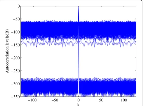
It can be observed that in all these figures, there exist two distinct ranges for the sidelobe distribution. This is because that for all algorithms, the optimal sequence is a local optimal solution. When the algorithms are initialized by random sequences, the generated sequence may reach global optimal (sequence with sidelobes that are less than −300 dB) or not. Comparing Figs.1,2, and3, we can see that the FCGA can generate the best sequence whose peak sidelobe level (PSL) is about−318 dB.
102 103 104
10 12 14 16 18 20 22 24
Sequence length N
Merit factor
(a)
CAN Accelerated MISL GD
FCGA
102 103 104
103 102 101 100 101 102
Sequence length N
Average running time (s)
(b)
CAN Accelerated MISL GD
FCGA
102 103 104
101 102 103 104
Sequence length N
Average iteration number
(c)
CAN Accelerated MISL GD
FCGA
102 103 104 101
102 103
Sequence length N
Merit factor
(a)
102 103 104
103 102 101 100 101 102
Sequence length N
Running time (s)
(b)
CAN Accelerated MISL GD FCGA
102 103 104
101 102 103 104
Sequence length N
Iteration number
(c)
CAN Accelerated MISL GD FCGA CAN
Accelerated MISL GD FCGA
Fig. 6 a–cThe performance metrics of different algorithms initialized by Frank sequence
To fully compare the sidelobe performance, we calculate the ISLs and PSLs of all 1000 sequences for each algorithm and record the running time of each trial. The cumula-tive distribution functions (CDF) of the ISLs, PSLs, and running time are presented in Fig.4. Since both ISL and PSL are the criterions related to the autocorrelation, the CDF of the ISLs and PSLs are similar as can be seen from Fig.4a,b. In Fig.4b, we can see that about 55.7% of the PSL of the FCGA sequences is less than−285 dB, while the PeCAN and ADMM algorithms are difficult to produce sequences with such PSL. Compared with the PeCAN, the overall sidelobe performance of the FCGA is better. The only drawback of the proposed algorithm is that about 41.8% of the PSLs of the FCGA sequences are located in [−100,−50] dB, while the ADMM has the proportion of only 10.3%. However, as shown in Fig. 4c, the running
time of the FCGA is about an order of magnitude smaller than that of the PeCAN and ADMM algorithms, which indicates the former is more computationally efficient. It is worth noting that since the ADMM is stopped after 2×10⁵iterations, the running time of ADMM is basically unchanged.
4.2 Aperiodic sequences design with low autocorrelation sidelobes
In this subsection, we investigate the performance of the proposed algorithm by designing aperiodic sequences (i.e., the case of λ = 0,N˜ = 2N). To show the advan-tage of the proposed algorithm, we compare the perfor-mance with several algorithms, including the CAN [9], the Accelerated-MISL [10], and the gradient descent (GD) algorithm in [23]. Among the three contrast algorithms,
102 103 104
101 102 103
Sequence length N
Merit factor
(a)
102 103 104
103 102 101 100 101 102
Sequence length N
Running time (s)
(b)
CAN Accelerated MISL GD FCGA
102 103 104
101 102 103 104
Sequence length N
Iteration number
(c)
CAN Accelerated MISL GD FCGA CAN
Accelerated MISL GD FCGA
−100 −50 0 50 100 −50
−45 −40 −35 −30 −25 −20 −15 −10 −5 0
k
Autocorrelation level(dB)
SCAN Spectral−MISL ADMM GD FCGA
Fig. 8Autocorrelation level of the sequences generated by five different algorithms
the CAN is the classical algorithm for this design problem, and the other two algorithms are proposed recently. All these algorithms are good at designing aperiodic sequence with low sidelobes and also have high computational effi-ciency. Since the ADMM is inferior to the CAN and Accelerated-MISL algorithms in terms of the aperiodic autocorrelation sidelobes [27], here we do not take the ADMM into account. The stopping criterion is set to be
xk+1−xk≤10−3for all algorithms.
In this experiment, we compare the quality of the designed sequences and the running times of these algo-rithms. Generally, the sequence quality can be measured by the merit factor (MF) (the large the better) which is defined as
0 0.2 0.4 0.6 0.8 1
−40 −35 −30 −25 −20 −15 −10 −5 0 5
Frequency (Hz)
Spectral power (dB)
SCAN Spectral−MISL ADMM GD FCGA
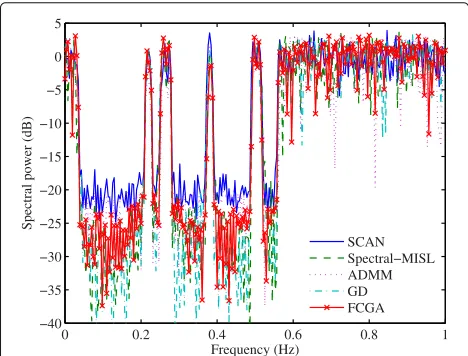
Fig. 9Spectral power of sequences generated by five different algorithms
MF= |r0|
2
2N−1 k=1
|rk|2
= N2
2ISL. (48)
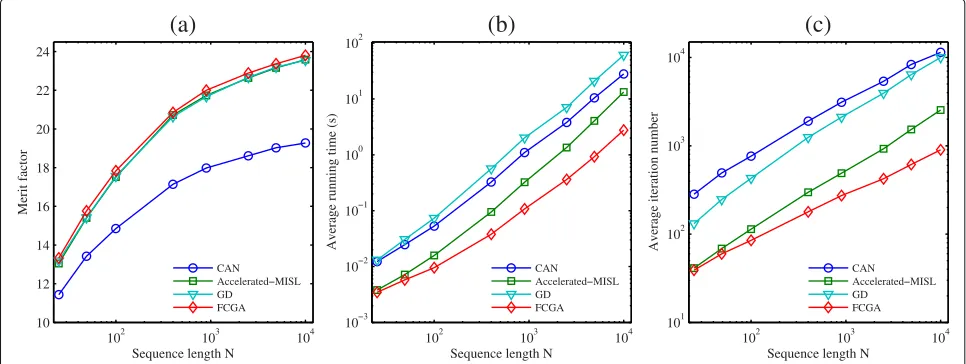
First of all, we use the random sequences to initialize the algorithms. To obtain the average values of the MF and running time, we repeat the four algorithms 300 times for each of the following lengths:N =25, 26, ..., 213. Figure5 shows the performance metrics (average merit factor, average running time, and average iteration number) of different algorithms. As we can see in Fig. 5a, the aver-age merit factors of the sequences designed by the FCGA, GD, and Accelerated-MISL are basically the same. This is because that these three algorithms are all gradient-based algorithms which are different from the CAN. Actually, the MF of the sequences designed by the FCGA is a lit-tle larger than that of the GD and Accelerated-MISL. From Fig.5b, it can be easily observed that the FCGA is faster than the other three algorithms, especially when the sequence length is very large. Although the FCGA costs a little more computations than the CAN and Accelerated-MISL algorithms at each iteration, the superiority of the FCGA comes from the reduction of the iteration num-ber. Figure5cshows the average iteration numbers of the four algorithms. From this figure, we can see that the average iteration number of the FCGA is the least. This may be because that (i) the FCGA minimizes the objective function (ISL) directly, rather than a more loose objective function which the Accelerated-MISL applied, and (ii) in our test, the step size of the FCGA seems more accurate than that of the GD in [23], which means that the FCGA has faster convergence speed. Taking the merit factor and the running time into account, the proposed FCGA is better than the other three algorithms.
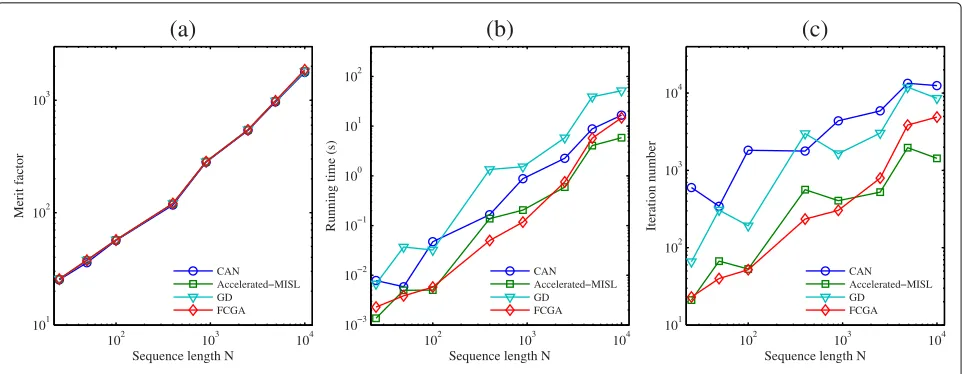
Next, we use the Frank sequence and Golomb sequence to initialize the four algorithms, and the results are shown in Figs. 6 and 7, respectively. It is well known that both the Frank sequence and the Golomb sequence have good autocorrelation property. Thus, after initializing by these two kinds of sequences, the algorithms can produce sequence with better sidelobe performance. In Figs. 6a and7a, the MF of different algorithms are almost the same and far greater than the result in Fig.5a. This indicates that the Frank sequence and Golomb sequence can lead to higher MF than the random sequence. Moreover, from Figs.6band7b, we can see that the FCGA is still an effi-cient and competitive algorithm when initialized by the Frank sequence or the Golomb sequence.
4.3 Sequence design with stopband property
18 17 16 15 14 13 12 11 10 0
0.2 0.4 0.6 0.8 1
PSL(dB)
CDF of PSL
SCAN Spectral MISL ADMM GD FCGA
24 22 20 18 16 14 12 10
0 0.2 0.4 0.6 0.8 1
PSP(dB)
CDF of PSP
SCAN Spectral MISL ADMM GD FCGA
102 103 104 105
0 0.2 0.4 0.6 0.8 1
iteration number
CDF of iteration number
SCAN Spectral MISL ADMM GD FCGA
102 101 100 101
0 0.2 0.4 0.6 0.8 1
running time(t)
CDF of running time
SCAN Spectral MISL ADMM GD FCGA
Fig. 10The cumulative distribution functions of the PSL, PSP, iteration number, and running time
The contrast algorithms are the SCAN [20], Spectral-MISL [10], ADMM, and GD [23] respectively, where the ADMM is the modified version for the synthe-sis of aperiodic unimodular sequences. Assume that the sequence length is N = 128, and the normal-ized frequency stopband considered here is [ 0.04, 0.21]∪ [ 0.23, 0.25]∪[ 0.28, 0.37]∪[ 0.39, 0.49]∪[ 0.52, 0.56]. In this experiment, we choosexk+1−xk ≤ 10−3as the
stop-ping criterion of the SCAN, Spectral-MISL, and FCGA algorithms. And the weight coefficientλ in these three algorithms are set to be 0.9, 104, 0.9, respectively. The parameters of the ADMM are the same as those in [27]. For the GD algorithm, we set the maximum iteration numberT =3000,αacf =0.1, andαspec=0.9.
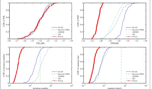
Figures8and9give an example of the autocorrelation level and spectrum power of the sequences designed by the five algorithms. The PSL of the sequences designed by the SCAN, Spectral-MISL, ADMM, GD, and FCGA algorithms are −14.01 dB, −14.09 dB, −15.64 dB, −13.80 dB, and −15.81 dB, respectively. And the corresponding peak stopband power (PSP) are−16.12 dB, −15.71 dB, −20.13 dB, −17.77 dB, and −20.73 dB. Like the other four algorithms, the proposed algorithm can suppress the autocorrelation sidelobes and the spectral power in frequency stopbands simultaneously.
Next, to eliminate the randomness, we repeat the algo-rithms 100 times and then record the PSL, PSP, itera-tion number NI, and running time t. Figure 10 shows the cumulative distribution functions of the four per-formance parameters (PSL, PSP,NI,t). And the average values of the parameters are provided in Table2. From Fig. 10 and Table 2, we can see that the PSL of these algorithms are basically the same, while the PSP of the ADMM and proposed algorithm (which have compara-ble performance) are lower than that of the other three algorithms. Moreover, the running time in Fig.10 indi-cates that the proposed algorithm is more computation-ally efficient than the other four algorithms owing to the fewer iterations.
Table 2Comparison of the performance parameters between the five algorithms
PSL (dB) PSP (dB) NI t(s)
5 Conclusions
In this paper, we have proposed an efficient algorithm named FCGA for designing periodic/aperiodic sequences with low autocorrelation sidelobes and low frequency stopband power. The FCGA algorithm is derived based on the conjugate gradient algorithm which can guarantee the monotonicity of the objective function. By changing the number of FFT points, the design of periodic and aperiodic sequences can be easily achieved. Since the main step of the FCGA can be implemented by FFT operations and Hadamard product, the proposed algorithm is com-putationally efficient and can be used to design sequences of large length. Several numerical experiments have been provided to demonstrate the superiority of the proposed algorithm.
Appendix 1: Derivation of phase gradient
By substituting (23) and (28) into (24), the gradient∇φJT can be rewritten as
∇φJT=2
where function| · |2is applied element-wise to the vector. According to (49) and (50),∇φJT can be expressed as tion, here we ignore the subscript ofFN˜). By substituting FforA, (51) can be rewritten as
Therefore, the phase gradient (52) can be implemented by FFT operations. Let
y=F−˜1
N
w◦FN˜(x)2◦FN˜ (x), (53)
then the phase gradient can be further simplified as ∇φJT =4N˜Re −jx∗◦y1:N
, (54)
wherey1:Ndenotes the firstNelements ofy.
Abbreviations
ADMM: Alternating direction method of multipliers; CAN: Cyclic algorithm new; CDF: Cumulative distribution function; CDMA: Code division multiple access; FCGA: FFT-based conjugate gradient algorithm; (I)DFT: (Inverse) discrete fourier transform; (I)FFT: (Inverse) fast fourier transform; ISL: Integrated sidelobe level; LFM: Linear frequency modulation; LPNN: Lagrange
programming neural network; MF: Merit factor; MISL: Monotonic minimizer for integrated sidelobe level; MM: Majorization-minimization; MMSE: Minimum mean square error; NAL: Normalized autocorrelation level; PeCAN:
Periodic-correlation cyclic algorithm new; PRP-CGA: Polak-Ribiere-Polyak-CGA; PSD: Power spectrum density; PSL: Peak sidelobe level; PSP: Peak stopband power; SCAN: Stopband cyclic algorithm new; SDCA: Steepest descent-based cyclic algorithm; WeCAN: Weighted cyclic algorithm new; WeSCAN: Weighted stopband cyclic algorithm new
Acknowledgements
The authors want to thank XiaoLi Sun for her great help in Latex editing and the anonymous reviewers for their valuable comments.
Funding
This work is supported by the Key Projects in the National Science & Technology Pillar Program during the Twelfth Five-year Plan Period (No. 2014BAK12B00) and the National Natural Science Foundation of China (No. 61101186 and No. 61101179).
Availability of data and materials
Please contact the author for data (Matlab codes) requests.
Authors’ contributions
LT conceived and devised the idea. LT and YZ designed and performed the experiments. YZ and QF analyzed the experiment results. All authors contributed to writing and editing the manuscript. All authors read and approved the final manuscript.
Competing interests
The authors declare that they have no competing interests.
Publisher’s Note
Springer Nature remains neutral with regard to jurisdictional claims in published maps and institutional affiliations.
Received: 30 March 2017 Accepted: 22 August 2018
References
1. S. W. Golomb, G. Gong,Signal design for good correlation: for wireless communication, cryptography, and radar. (Cambridge University Press, Cambridge, 2005)
2. H. He, J. Li, P. Stoica,Waveform design for active sensing systems: a computational approach. (Cambridge University Press, Cambridge, 2012) 3. N. Levanon, E. Mozeson,Radar signals. (Wiley, New York, 2004)
4. D. Tse, P. Viswanath,Fundamentals of wireless communication. (Cambridge University Press, New York, 2005)
6. W. H. Mow, K. L. Du, W. H. Wu, New evolutionary search for long low autocorrelation binary sequences. IEEE Trans. Aerosp. Electron. Syst.51(1), 290–303 (2015)
7. C. J. Nunn, G. E. Coxson, Polyphase pulse compression codes with optimal peak and integrated sidelobes. IEEE Trans. Aerosp. Electron. Syst.45(2), 775–781 (2009)
8. P. Borwein, R. Ferguson, Polyphase sequences with low autocorrelation. IEEE Trans. Inf. Theory.51(4), 1564–1567 (2005)
9. P. Stoica, H. He, J. Li, New algorithms for designing unimodular sequences with good correlation properties. IEEE Trans. Signal Process.57(4), 1415–1425 (2009)
10. J. X. Song, P. Babu, D. P. Palomar, Optimization methods for designing sequences with low autocorrelation sidelobes. IEEE Trans. Signal Process. 63(15), 3998–4009 (2015)
11. F. C. Li, Y. N. Zhao, X. L. Qiao, A waveform design method for suppressing range sidelobes in desired intervals. Signal Process.96, 203–211 (2014) 12. J. X. Song, P. Babu, D. Palomar, Sequence design to minimize the
weighted integrated and peak sidelobe levels. IEEE Trans. Signal Process. 64(8), 2051–2064 (2016)
13. H. Wu, Z. Y. Song, H. Q. Fan, Q. Fu, Designing sequence with low sidelobe levels at specified intervals based on psd fitting. Electron. Lett.51(1), 99–100 (2015)
14. P. Stoica, H. He, J. Li, On designing sequences with impulse-like periodic correlation. IEEE Signal Process. Lett.16(8), 703–706 (2009)
15. A. Aubry, A. De Maio, Y. Huang, M. Piezzo, A. Farina, A new radar waveform design algorithm with improved feasibility for spectral coexistence. IEEE Trans. Aerosp. Electron. Syst.51(2), 1029–1038 (2015) 16. W. Rowe, P. Stoica, J. Li, Spectrally constrained waveform design. IEEE
Signal Process. Mag.31(3), 157–162 (2014)
17. M. J. Lindenfeld, Sparse frequency transmit and receive waveform design. IEEE Trans. Aerosp. Electron. Syst.40(3), 851–861 (2004)
18. Z. T. Luo, K. Lu, X. Y. Chen, Z. S. He, Wideband signal design for over-the-horizon radar in cochannel interference. Eurasip J. Adv. Signal Process.2014(1), 159 (2014)
19. P. Ge, G. L. Cui, L. J. Kong, J. Y. Yang, Unimodular sequence design under frequency hopping communication compatibility requirements. Eurasip J. Adv. Signal Process.2016(1), 137 (2016)
20. H. He, P. Stoica, J. Li, in2nd International Workshop on Cognitive Information Processing (CIP) 2010. Waveform design with stopband and correlation constraints for cognitive radar (IEEE, Elba, 2010), pp. 344–349 21. G. Wang, Y. Lu, Designing single/multiple sparse frequency waveforms
with sidelobe constraint. IET Radar Sonar Navig.5(1), 32–38 (2011) 22. H. Wu, Z. Y. Song, H. Q. Fan, Y. X. Li, Q. Fu, A new algorithm for sparse
frequency waveform design with range sidelobes constraint. Chinese J. Electron.24(3), 604–610 (2015)
23. B. O’Donnell, J. M. Baden, in2016 IEEE Radar Conference. Fast gradient descent for multi-objective waveform design (IEEE, Philadelphia, 2016), pp. 1–5
24. D. Zhao, Y. Wei, Y. Liu, Spectrum optimization via FFT-based conjugate gradient method for unimodular sequence design. Signal Process.142, 354–365 (2018)
25. J. L. Liang, H. C. So, C. S. Leung, J. Li, A. Farina, Waveform design with unit modulus and spectral shape constraints via Lagrange programming neural network. IEEE J. Sel. Topics Signal Process.9(8), 1377–1386 (2015) 26. X. Feng, Y. C. Song, Z. Q. Zhou, Y. N. Zhao, Designing unimodular
waveform with low range sidelobes and stopband for cognitive radar via relaxed alternating projection. Int J Antennas Propag.2016, 1–9 (2016) 27. J. L. Liang, H. C. So, J. Li, A. Farina, Unimodular sequence design based on
alternating direction method of multipliers. IEEE Trans. Signal Process. 64(20), 5367–5381 (2016)