Generalization of interpolation DFT algorithms and frequency estimators with high image component interference rejection

(1)

R E S E A R C H

Open Access

Generalization of interpolation DFT

algorithms and frequency estimators

with high image component interference

rejection

Jiufei Luo

1*

, Shuaicheng Hou

2

, Xinyi Li

3

, Qi Ouyang

2

and Yi Zhang

1

Abstract

This paper focuses on the problem of frequency estimation of noise-contaminated sinusoidal. A basic tool to solve this problem is the interpolated discrete Fourier transform (DFT) algorithms, in which the influences of the spectral leakage from negative frequency are often neglected, resulting in significant errors in estimation when the signals contained small cycles. In this paper, analytic expressions of the interference due to the image component are derived and its influences on the traditional two-point interpolated DFT algorithms are analyzed. Based on the achieved expressions, the interpolated DFT algorithms are generalized and a novel frequency estimator with high image component interference rejection is proposed. Simulation results show that the frequency errors returned by the new algorithm are very small even though only one or two cycles are obtained. Comparative studies indicate that the new algorithm also has a good performance in the noise condition. With the advantages of high precision and strong robustness against additive noise, the proposed algorithm is a good choice for frequency estimation when the negative frequency interference is the dominant error source.

Keywords:Frequency estimation, Discrete Fourier transform, Spectral leakage, Image frequency interference

1 Introduction

Spectral analysis based on the discrete Fourier form (DFT) and implemented by the fast Fourier trans-form (FFT) has been widely used in many fields for several decades. However, there are two drawbacks in the classic version: the spectral leakage effect (SLE) caused by the lack of periodicity and the picket fence effect (PFE) due to the frequency sampling [1]. These effects will lead to significant errors in spectral analysis such as parameter estimation [2, 3]. In order to obtain accurate estimates of signal parameters, a lot of solu-tions were proposed [4–14]. The interpolation discrete Fourier transform (IpDFT) algorithm is one of the most popular algorithms.

Early in 1970s, interpolation algorithms based on the moduli of two FFT spectral bins were presented by Rife et al. [4]. Various improved algorithms have been put forward in the following decades, such as the weighted interpolated DFT (WIDFT) proposed by Agrez [9] and the multi-point interpolated DFT approach (WMlpDFT) by Belega and Dallet [12]. Specifically, simple analytical solutions can be obtained when the maximum sidelobe decay windows (MSDW, also known as Rife–Vincent class I windows) are adopted [11]. However, the algo-rithms mentioned above are all established on a very im-portant assumption that the leakage coming from the image component plays a minor role and could be ig-nored [11–13]. In fact, if signals contain a small number of cycles, the negative frequency component usually will exercise great influences on the estimators [15]. Al-though the multi-point IpDFT methods can reduce the sensitivity to some extent, frequency estimation errors due to the spectral interference from the image compo-nent still remain significant [15], especially for the * Correspondence:[email protected]

1_{School of Advanced Manufacture Engineering, Chongqing University of} Posts and Telecommunications, Chongqing 400065, People_’s Republic of China

Full list of author information is available at the end of the article

(2)

signals with a few cycles. Furthermore, it should be em-phasized that the reduction of systematic errors by the weighted interpolated DFT or multi-point IpDFT methods is at the expense of worse noise properties [9, 12]. In en-gineering practice, noise properties usually are more im-portant than systematic errors. The accuracy could be improved with longer records as well, but the cost is in-creased response time [16]. As a result, we often have to make a tradeoff between the estimation accuracy and the overall system responsiveness. Consequently, it is of great significance to propose a new and simple algorithm by which accurate parameter estimates can be achieved with short intervals, especially for those fields where real-time response is required [16–18].

Recently, Belega et al. proposed an improved three-point IpDFT which exhibits a high rejection capability with respect to the interference from negative quency [15]. In this paper, we proposed a novel fre-quency estimator by which the leakage coming from image component can be further reduced compared with the algorithm proposed by Belega et al. More im-portantly, it also keeps good noise properties due to a two-point-based mechanism. The remaining parts are organized as follows. In Section 2, we present a concise summary of the traditional interpolation algorithms. Symbols and basic equations used throughout the paper are defined in this section as well. In Section 3, the analytical expressions of the interference from the negative frequency are derived. With the properties of the derived expressions, we generalize the interpolation DFT algorithms. In Section 4, the frequency estimators with high interference rejection of image component are pro-posed. In Section 5, some computer simulations are carried out and the performance of the proposed algo-rithms are compared with some other state-of-the-art IpDFT methods. Finally, main conclusions are drawn in Section 6.

2 Theoretical background

In order to explain the basis of the frequency-estimating procedure, first, let xraw(n) be the samples of a discrete cosine wave in the form

xrawð Þ ¼n A0 cos 2πð f0nΔTþφ0Þ n¼0;1;2;…

ð1Þ

where A0, f0, and φ0 are the amplitude, frequency, and

phase, respectively. ΔT denotes the sampling interval and nis the index of the samples. Sampling rate fs= 1/

ΔT is supposed to fulfill the Nyquist sampling theorem so that aliasing of spectrum does not occur. When N samples are acquired, f0 is normalized by the frequency resolutionΔf=fs/Nand is expressed as

λ0¼_Δf0_f ¼_ff0

s=N; ð

2Þ

where λ0 is the normalized frequency expressed in bins

[12]. Usually, samples are weighted by a window func-tionwN(n) before DFT

x nð Þ ¼xrawð ÞnwNð Þn ð3Þ

The DFT ofN weighted samples at the spectral linek is given by

the bin number with the largest magnitude isl, then the largest magnitude is given by

X lð Þ

The second largest magnitude is given by

X lð 1Þ

represent the image component in the spectrum. The interference is very small compared with the first term as long asl is far from zero frequency and Nyquist fre-quency. In this situation, W_N(l+λ0) can be ignored and

(5) is reduced to

X lð Þ j j ¼A0

2 jWNðl−λ0Þj ð7Þ

Similarly, (6) can be rewritten as

X lð 1Þ

j j≅A0

2 jWNðl−λ01Þj ð8Þ

For the two-point (2p) interpolation algorithm [6, 8, 11], we introduce α defined as the ratio of the two lar-gest magnitudes

α¼jX l_jð_{X l}_{ð Þ}_j1Þj≅WNðl−λ01Þ

WNðl−λ0Þ ð

9Þ

It can be clearly seen from Eq. (9) that the ratioαonly depends on the normalized frequencyλ0if the data

win-dow is already known. In particular, λ0 can be

(3)

λ0¼lHα−Hþ

1

αþ1 ð10Þ

In (10), Hdenotes the number of terms in the max-imum sidelobe decay window. For other windows, λ0

can be obtained by the polynomial approximation method [13].

Similarly, with proper combination of three or more spectral lines, a ratio α can be obtained which only de-pends on the selected window and λ0 [9, 12]. Once the

data window is chosen,λ0can be solely determined byα,

λ0¼hð Þα ð11Þ

If the maximum sidelobe decay windows are selected, αcan be obtained from (10). Once αis determined, the normalized frequency can be computed and the fre-quency can be worked out in Eq. (2).

As shown above, the second terms on the right in Eqs. (5) and (6) representing the interferences from the image component in the spectrum have been neglected. The approximation will be reasonable if λ0> 5 and λ0<N/2 −5. However, ifλ0were out of the specified ranges,

sig-nificant errors would be generated [15]. Therefore, it is of great importance and necessary to deduce a simple al-gorithm that is applicable even when λ0 is in the

ex-treme ranges.

3 Generalization of interpolation DFT algorithms In Section 2, it was already known that

X lð Þ ¼A0

It should be pointed out that due to the actual pro-cessing requirements of causality, w_N(n) is a time-shifting window, where n= 0, 1⋅ ⋅ ⋅N−1. It can be ob-tained by

wNð Þ ¼n w nð −N=2Þ ð14Þ

w(n) is assumed to be a DFT-even window [2], which is symmetric with respect to the origin. According to the time-shifting property of DFT, we have

WNð Þ ¼k W kð Þe−jkπ; ð15Þ

where W(k) is the DTFT of the window w(n) and the complex exponential factor corresponds to the time shift. W(k) is also symmetric and real because w(n) is symmetric and real. Substituting Eq. (15) into Eq. (12),

X(l) can be rewritten as

Because the period of the complex sinusoidal is 2π, Eq. (16a) can be further expressed as

X lð Þ ¼A0

The real and imaginary parts are expressed as

XRðlÞ ¼A0

Now, we introduce two variablesαR,αIdefined as

αR¼ XR_Xðl1Þ

It is assumed, similar to that in Section 2, thatλ0is far

enough from the origin so that the leakage terms W(2l +δ) andW(2l+δ± 1) are very small compared toW(−δ) and W(−δ± 1) and could be ignored. With this assump-tion, we can get the following relationship

αR≅αI≅α≅W_Wð−_{ð Þ}δ₋_δ 1Þ ð20Þ

(4)

In other words, the frequency estimate only depends on the frequency itself.

We proceed to analyze the traditional algorithm without making approximation. The moduli of X(l) and X(l± 1) can be obtained by the square roots ofJ(l) andJ(l +1), re-spectively, according to the results in Eqs. (17a), (17b), (18a), and (18b).

J lð Þ ¼A20

4 W

2_{ð Þ þ}₋_δ _W2_ð₂_l_þ_δ_Þ

þA20

2 cos 2φð 0þ2δπÞWð Þ−δ Wð2lþδÞ

ð21aÞ

J lð 1Þ ¼A

2 0

4 W

2_ð₋_δ₁_{Þ þ}_W2_ð₂_l_þ_δ₁_Þ

þA20

2 cos 2ð φ0þ2δπÞWð−δ1ÞWð2lþδ1Þ ð21bÞ

Without making approximation, Eq. (10) becomes

α¼jX l_jð_{X l}_{ð Þ}1_jÞj¼

ffiffiffiffiffiffiffiffiffiffiffiffiffiffiffiffi J lð 1Þ p

ffiffiffiffiffiffiffiffi J lð Þ

p ð22Þ

Obviously, α is phase dependent. Also, for Hanning window, (namely two-term MSD window) it can be proved that (see Appendix 1)

λR≥λ≥λI; ð23Þ

whereλR,λI, andλare corresponding estimation values

by αR,αI and α. If δ≠0, the first equality sign is only

forφ0+δπ= 0 orπand the second equality sign is only

for φ0+δπ= ±π/2. Systematic error will be introduced

no matter which of the three ratios is used in formula (11). The difference is that αR is only affected by the

real part of negative frequency and αI is only affected

by the imaginary part of the negative frequency compo-nent, while α is affected by both the real and imaginary parts.

Inspired by modulus-based ratio, we can extend the ratio to a more general notation. With a proper combin-ation of the real and imaginary parts ofX(l) andX(l± 1), we can get various kinds of ratios. For example,^αcan be defined as

^

α¼jXRðl_X1Þ þj jXIðl1Þj Rð Þ þl j jXIð Þl

j j ð24Þ

Similar toα, we have

^

α≅Wð−δ1Þ

WNð Þ−δ ; ð25Þ

and for Hanning window, we can also obtain

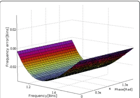
Fig. 1Frequency estimation errors when Hanning window is

used (α=αR)

used (α=αI)

(5)

λR≥^λ≥λI; ð26Þ

where ^λ is estimation value by α^. It is indicated that a new estimator can be obtained if α in formula (11) is replaced byα^. The proof of Eq. (26) is similar to that of Eq. (23). Frequency estimation errors of the four estima-tors when 1 <λ0< 2 (samples are weighted by Hanning

window) are shown in Figs. 1, 2, 3, and 4. In Figs. 1 and 2, it can be seen that for a certain frequency, the fre-quency error is constant in spite of the variable phase. It is confirmed that the frequency estimators, based on the αR,αI separately, are independent of the signal phase,

while the estimators based on α;^α are the functions of both the frequency and the phase. Comparing the esti-mated errors in Figs. 1, 2, 3, and 4, we can also see that the simulation results coincide well with the theoretical analysis in Eqs. (23) and (26). The difference between the two estimators in Figs. 3 and 4 is that the developing trend of errors in Fig. 3 is smoother than that in Fig. 4. We now have to emphasize again that maximum abso-lute errors are obtained when the phase and the offset satisfy the relationshipφ0+δπ= 0 orφ0+δπ=π/2. For a

certain offset, the maximum error is equal to the error

shown in Figs. 1 and 2. In addition, we can also construct other types of ratio to create new estimators by combining the real and imaginary parts ofX(l) andX(l± 1) properly.

4 Algorithms with high image component interference rejection

As we can see in Figs. 1, 2, 3, and 4, the maximum error due to negative frequency can reach as high as 0.04 for all the estimators. Simulation results show that it can be even up to nearly 0.1 for the rectangle window and up to 0.2 for the three-term maximum decay window. As a result, it is of great significance to reduce the interfer-ence resulting from the negative frequency. A new inter-polated algorithm which has strong resistance against interference from the negative frequency component is proposed in this section.

4.1 Simple algorithms with high image component interference rejection

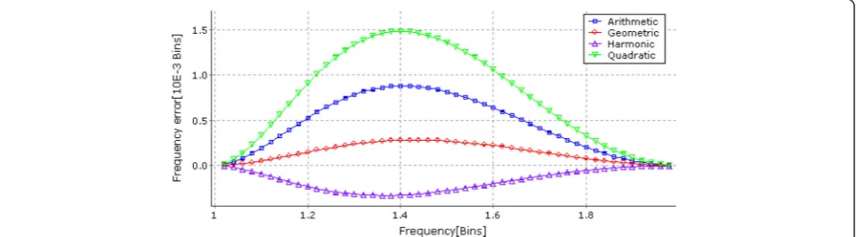
Recalling Eqs. (19a) and (19b) and observing Figs. 1 and 2, we can infer that there is nearly a complemen-tary relationship between the two estimators. A proper combination of the two estimators can probably result in an intrinsic rejection of negative frequency leakage. Hence, we introduce α1defined as the arithmetic mean

value ofαRandαI,

α1¼ðαRþαIÞ=2

¼Wð−δ1Þ−Wð2lþδ1ÞWð2lþδÞ=Wð Þ−δ Wð Þ−δ −W2_ð₂_l_þ_δ_Þ₌_W_{ð Þ}₋_δ

ð27aÞ

Now, the interference terms areW(2l+δ± 1)W(2l+δ)/

W(−δ) andW2(2l+δ)/W(−δ), much smaller than the ori-ginal terms W(2l+δ± 1) and W(2l+δ). Most errors are eliminated by a simple arithmetic average operation. Simi-larly, we can also introduce α2, α3, andα4defined as the

geometric mean value, the harmonic mean value, and the quadratic mean ofαRandαI, respectively, as indicated in

used (α¼^α)

(6)

α2¼pffiffiffiffiffiffiffiffiffiffiαRαI ¼

ffiffiffiffiffiffiffiffiffiffiffiffiffiffiffiffiffiffiffiffiffiffiffiffiffiffiffiffiffiffiffiffiffiffiffiffiffiffiffiffiffiffiffiffiffiffiffiffiffiffiffiffiffiffiffiffiffiffiffi W2_ð₋_δ₁_Þ₋_W2_ð₂_l_þ_δ₁_Þ

W2_{ð Þ}₋_δ ₋_W2_ð₂_l_þ_δ_Þ

s

;

ð27bÞ

α3 ¼

2 1=αRþ1=αI ¼

α2 2

α1; ð

27cÞ

and

α4 ¼

ffiffiffiffiffiffiffiffiffiffiffiffiffiffiffiffiffiffiffiffiffiffiffiffiffi α2

Rþα2I

=2 q

¼ ffiffiffiffiffiffiffiffiffiffiffiffiffiffiffi2α2₁₋_α2 2

q

ð27dÞ

Similar to α1, the interference terms of α2 become

much smaller as well.α3andα4can be written as simple

functions of α1 and α2, respectively. The values of the

four means are approximately equal. To demonstrate the ability of negative frequency leakage rejection, the fre-quency errors of the four estimators are displayed when 1 <λ0< 2. Note that the four estimators are also phase

independent because no phase information is involved in the ratios shown in Eqs. (27a)–(27d). Consequently, the phase was just set to zero. Figures 5 and 6 show the

estimation results as a function of the frequency. It can be seen that the frequency errors sharply decrease com-pared with the modulus-based algorithms. In particular, the remaining error for the one based on the harmonic mean value is less than 10−3, which is small enough for the engineering practice.

4.2 Further improved interpolation algorithms with slide DFT

However, there is a serious defect in the above rithms in which the weighed ratio is used. The algo-rithms may become quite vulnerable if cos(φ0+δπ)≈0

or sin(φ0+δπ)≈0. Under such two circumstances, the

imaginary parts or the real parts would be so small that even a small disturbance would lead to a dramatic change in αR or αI, resulting of significant errors in the

final frequency estimates. Theoretical cosine waves cor-rupted by low-level random noise were generated to con-firm the defect, and the vulnerability of two frequency estimators based on αRandαIis shown in Figs. 7 and 8,

respectively. It is clearly shown that radical changes ap-pear when cos(φ0+δπ)≈0 forαRand sin(φ0+δπ)≈0 for

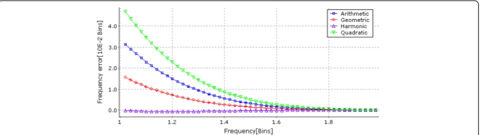
Fig. 6Frequency estimation errors based on different means ofαRandαIwhen three-term MSD window is used

Fig. 7The phenomenon of“Luo–arêtes”in theαR-based estimator

(Hanning window)

Fig. 8The phenomenon of“Luo–arêtes”in theαI-based estimator

(7)

αI. Sharp peaks along these lines are observed in the

sur-face of the frequency errors. They look like knife-edge arêtes so we call them “Luo–arêtes.” In contrast, for the frequencies that are not in the vicinity of these lines, er-rors are very small and remain stable.

To avoid the “Luo–arêtes,”a further improved algo-rithm has been proposed. The fact that αR andαI

(in-cluding various kinds of mean values of the two) are phase independent and the change of phase has no in-fluences on frequency estimates help us get a robust ratio by time-shifting technique. Now, consider a discrete sequence with N samples x(0),x(1)⋅ ⋅ ⋅x(N−1) and assume that its observed phase is φ1. After delaying

forL samples, we get a time-shifted sequencex(L),x(L+ 1)⋅ ⋅ ⋅x(N+L−1) and its observed phase φ2 can be

expressed as

φ2¼φ1þ2πf0LΔT¼φ1þ2πf0L=fs¼φ1þ2πλ0L=N

ð28Þ

In the above equation,ΔTis the sampling interval,f0is the theoretical frequency and λ0 is the normalized

fre-quency scaled by frefre-quency resolution. Asλ0is unknown,

we can use its largest bin numberl,instead.

L≈Nφ2−φ1

2πl ð29Þ

The actual observed phase of the time delay sequence isφ'2=φ1+ 2πlL/Nand the phase error is

φ20−φ2¼Δφ2¼2πδL=N ð30Þ

Generally, we havel> 1 and φ2−φ1<π/2 so thatL/N

< 1/4. Considering δ∈[−0.5, 0.5), the absolute phase error is less thanπ/4. Forα_R, ifφ2was set to 0 orπ,φ'2

was limited in the range of (−π/4,π/4) or (3π/4, 5π/4). Forα_I, ifφ2was set toπ/2 or −π/2,φ'2was limited in

the range of (π/4, 3π/4) or (−3π/4,−π/4). It is indicated that we can adjust the observed phase by the time-shifting technique so that we can get a robust ratio to avoid the “Luo–arêtes.” In addition, we can obtain the spectral lineslandl ±1 of the time-delayed sequence by means of the sliding discrete Fourier transform (SDFT) [19, 20]. It will be more efficient compared with another separate FFT or DFT.

5 Comparison with other state-of-the-art methods In this section, some computer simulations were con-ducted to verify the effectiveness and the accuracy of the proposed algorithms. For conciseness, only the results of

Fig. 9Maximum estimation error as a function of_λ0for different estimators without noise (Hanning window)

(8)

the algorithm based on the harmonic mean of α_R and α_I were shown. All simulation results are returned by the al-gorithm proposed in Section 4.2. In addition, the results of the traditional IpDFT algorithm (2pIpDFT) [5, 8, 11], the classical three-point IpDFT algorithm (3pIpDFT) [9, 12], Quinn’s two-point-based estimator (Quinn1, only applic-able for Hanning window), and Quinn’s three-point-based optimal estimator (Quinn2, only applicable for Hanning window) [21–23], the estimator proposed by Macleod in 1998 (Macleod, only applicable for Hanning window) [24], the three-point complex spectrum-based estima-tor (Jacobsen, only applicable for Hanning window) [25] referred by Jacobsen and Kootsookos in 2007, and the improved three-point IpDFT algorithm with high image frequency interference rejection capability re-cently proposed by Belega (Belega14) [15], were also displayed for comparison. In all the considered IpDFT-based algorithms, both the two-term and three-term MSD windows were adopted. For simplicity but without loss of generality, parameters used in all the simulation experiments were as follows, the amplitude of the cosine waveA= 1, the number of samplesN =512, and the sam-pling ratef_s= 512. The results shown in this section were scaled by frequency resolution and expressed in bins.

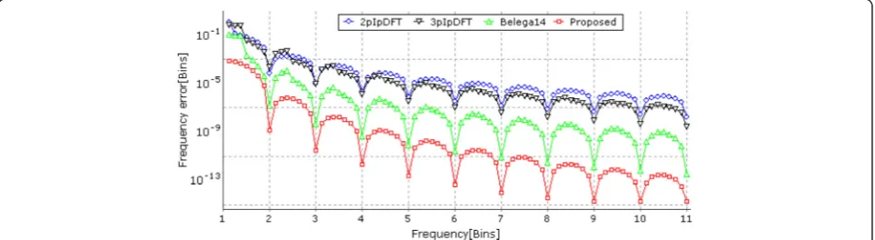
5.1 Theoretical cosine wave without noise

To demonstrate the excellent rejection capability against the interference from negative frequency, theoretical sig-nals contain a small number of cycles. The normalized frequencyλ0is varied in the range (1, 11) with a step of

1/8. For each frequency, the phase θ is varied in the range [−π, π) with a step of π/72. The maximum abso-lute frequency errors |δ|maxare shown in Figs. 9 and 10

as a function of λ0 for the two-term and three-term

MSD windows, respectively. It is clearly revealed that the errors due to negative frequency interference are re-markably reduced. In general, both the proposed method and the improved three-point IpDFT method outperform other estimators throughout the entire range of consid-eredλ0. When the Hanning window is adopted, Jacobsen’s

estimator has the worst performance. The traditional IpDFT algorithm, Quinn’s two-point-based estimator, and Quinn’s three-point-based optimal estimator have similar trend. The classical three-point IpDFT algorithm and Macleod’s estimator provide better results than the above three estimators. If λ0< 4.5 (especiallyλ0< 1.5) andδ> 0,

the new method provides better performance than the im-proved three-point IpDFT and the opposite holds ifδ<0. When λ0> 4.5, the improved three-point IpDFT shows a

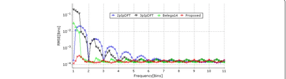
Fig. 11RMSE for different algorithms (SNR = 30 dB, Hanning window)

(9)

small advantage than the proposed algorithm. When the three-term MSD window is adopted, the new estimator has overwhelming advantage over the rest. It should be pointed out that regardless of the adopted window type and the value ofλ0, the maximum frequency error of the

new algorithm never goes above 10−3, even though only one or two cycles are obtained.

5.2 Theoretical cosine wave corrupted by additive noise In this subsection, we considered the ideal cosine wave contaminated with the additive Gaussian noise. Similar to [15], we investigated the RMSE of estimates returned by the considered estimators as a function ofλ0for

cer-tain SNRs. For each frequency, 50,000 instances were generated with a random phase. For conciseness, four algorithms are considered, including the traditional IpDFT algorithm (2pIpDFT), the classical three-point IpDFT algorithm (3pIpDFT), the improved three-point IpDFT algorithm with high image frequency interfer-ence rejection capability (Belega14), and the proposed algorithm. Results with SNR = 30 dB and 50 dB for Hanning window and three-term MSD window were shown in Figs. 11, 12, 13, and 14, respectively. The re-sults for Hanning window agree well with those in [15]. As shown in Figs. 11 and 12, the estimated RMSE of the proposed method is always in a low level with a small

fluctuation and essentially the novel method has no com-petitor for λ0< 3. Whenλ0becomes larger, the estimated

RMSE of four estimators tend to be in a similar level and it is interesting to find that the two-point-based algo-rithms show a better performance at the worst incoherent sampling condition (δ≈0.5), while the three-point-based algorithms provide better results whenλ0is close to

inte-ger values (δ≈0).

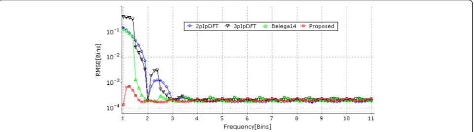
When the three-term MSD window is adopted, the overall trend is similar to that of Hanning window. For λ0< 2, the performance of the traditional 2pIpDFT and

3pIpDFT is worse than Hanning window due to the wider mainlobe of the three-term MSD window. For λ0> 2, they have better performances because of the

faster sidelobe decay rate. For the same SNR, the RMSE values of the two algorithms employing three-term MSD window decrease faster than that employing Hanning win-dow before reaching the ultimate stable level. Meanwhile, the ultimate stable level is higher than that employing Hanning window because of the worse noise properties of the three-term MSD window. The performance of the proposed algorithm maintains its superiority to the other three algorithms for λ0< 3. To sum up, the traditional

two-point- or three-point-based algorithms are very good choices because of their simplicity when random noise has a significant influence on the uncertainty of estimates.

Fig. 13RMSE for different algorithms (SNR = 30 dB, three-term MSD window)

(10)

The proposed algorithm is strongly recommended when the image frequency interference is the main error source especially when a small number of cycles are contained in samples.

6 Conclusions

Frequency estimation by the IpDFT method is studied in this paper. We have quantitatively analyzed the influ-ences of the interference from the image component and generalized the interpolated DFT algorithms. Based on the analysis, novel frequency estimators are proposed, which have strong rejection against the high image com-ponent interference. Accuracy of the novel algorithm has been confirmed by simulations. Comparative studies reveal that the proposed algorithm has a better perform-ance than the traditional algorithms when the spectral interference from negative frequency component is sig-nificant, especially for the cycles less than one and a half. This proposed algorithm is simple to understand, easy to implement, and very suitable for real-time analysis.

7 Appendices 7.1 Appendix 1

According to the conclusion in Eq. (10), we can get the frequency estimation by

λ¼l_α2α_þ−1

1; ðA1Þ

when Hanning window is used.

Accordingly, we can obtain frequency estimations

λR¼l_α2αR−1

Further, combining Eq. (A2a) with Eq. (A2c) and Eq. (A2b) with Eq. (A2c), we get the following two equations

^

The above equations indicate the following conclusions.

(1)Forδ> 0, sinceαR>α,αI <α(Appendix 2) and it

from Section 3, where W0=

W(−δ),W1=W(−δ± 1),W2_l=W(2l+δ),W2_l+ 1=W(2l

+δ± 1) and u= cos(2φ0+ 2δπ) according to Eqs. (19a),

(19b), and (22). We define

E¼α2

After some algebraic manipulation, we obtain

E¼2 1ð −uÞ G

When Hanning window is used, we know that W0>

(11)

(1)Forδ> 0, we haveW2l< 0 andW2l+ 1> 0 for Hanning

window, soG> 0. Then, we haveαR>αandαI <α.

(2)Forδ< 0, we haveW2l> 0 andW2l+ 1< 0 for Hanning

window, soG< 0. Then, we haveαR<αandαI >α.

It should be pointed that forδ≠0, the requirement for αR¼α is thatμ= 1 and the requirement for αI ¼α is thatμ=−1. That means thatφ0+δπ= 0 orπforαR¼α

andφ0+δπ= ±π/2 forαI ¼α.

Competing interests

The authors declare that they have no competing interests.

Acknowledgements

The authors want to thank the anonymous reviewers for their helpful comments, which significantly improved the quality of the paper. This research was supported by the Science Foundation for Young Scientists (Grant No. E010A2015063) and Startup Fund for Doctors (Grant No. E010A2015037) of Chongqing University of Posts and Telecommunications, Chongqing Science and Technology Commission (Grant No. cstc2015jcyjB0241) and also was partly supported by the National Natural Science Foundation of China (Grant No. 51374264).

Author details

1_{School of Advanced Manufacture Engineering, Chongqing University of} Posts and Telecommunications, Chongqing 400065, People_’s Republic of China.2_{School of Automation, Chongqing University, Chongqing 400044,} People’s Republic of China.3Department of Mechanical Engineering, Chongqing University, Chongqing 400044, People’s Republic of China.

Received: 25 August 2015 Accepted: 24 February 2016

References

1. KF Chen, JT Jiang, S Crowsen, Against the long-range spectral leakage of the cosine window family. Comput Phys Commun180, 904–911 (2009) 2. FJ Harris, On the use of windows for harmonic analysis with the discrete

Fourier transform. Proc IEEE66, 51–83 (1978)

3. J Luo, M Xie, Phase difference methods based on asymmetric windows. Mech Syst Signal Process54, 52–67 (2015)

4. DC Rife, G Vincent, Use of the discrete Fourier transform in the measurement of frequencies and levels of tones. Bell Syst Tech J49, 197–228 (1970) 5. VK Jain, WL Collins, DC Davis, High-accuracy analog measurements via

interpolated FFT. Instrumentation and Measurement, IEEE Transactions on

28, 113–122 (1979)

6. T Grandke, Interpolation algorithms for discrete Fourier transforms of weighted signals. Instrumentation and Measurement, IEEE Transactions on

32, 350–355 (1983)

7. M Xie, K Ding, Corrections for frequency, amplitude and phase in a fast Fourier transform of a harmonic signal. Mech Syst Signal Process10, 211–221 (1996) 8. J Luo, Z Xie, M Xie, Frequency estimation of the weighted real tones or

resolved multiple tones by iterative interpolation DFT algorithm. Digital signal processing41, 118–129 (2015)

9. D Agrez, Weighted multipoint interpolated DFT to improve amplitude estimation of multifrequency signal. Instrumentation and Measurement, IEEE Transactions on51, 287–292 (2002)

10. J Luo, Z Xie, M Xie, Interpolated DFT algorithms with zero padding for classic windows. Mech Syst Signal Process70–71, 118–129 (2016) 11. D Belega, D Dallet, Multifrequency signal analysis by Interpolated DFT method

with maximum sidelobe decay windows. Measurement42, 420–426 (2009) 12. D Belega, D Dallet, D Petri, Accuracy of sine wave frequency estimation by

multipoint interpolated DFT approach. Instrumentation and Measurement, IEEE Transactions on59, 2808_–2815 (2010)

13. J-R Liao, C-M Chen, Phase correction of discrete Fourier transform coefficients to reduce frequency estimation bias of single tone complex sinusoid. Signal Process94, 108–117 (2014)

14. J-R Liao, S Lo, Analytical solutions for frequency estimators by interpolation of DFT coefficients. Signal Process100, 93–100 (2014)

15. D Belega, D Petri, D Dallet, Frequency estimation of a sinusoidal signal via a three-point interpolated DFT method with high image component interference rejection capability. Digital Signal Processing24, 162–169 (2014) 16. D Belega, D Petri, Accuracy analysis of the multicycle synchrophasor

estimator provided by the interpolated DFT algorithm. IEEE Trans Instrum Meas62, 942_–953 (2013)

17. P Castello, M Lixia, C Muscas, PA Pegoraro, Impact of the model on the accuracy of synchrophasor measurement. Instrumentation and Measurement, IEEE Transactions on61, 2179–2188 (2012)

18. Y Tu, H Zhang, Method for CMF signal processing based on the recursive DTFT algorithm with negative frequency contribution. Instrumentation and Measurement, IEEE Transactions on57, 2647–2654 (2008)

19. E Jacobsen, R Lyons, The sliding DFT. Signal Processing Magazine, IEEE20, 74_–80 (2003)

20. K Duda, Accurate, guaranteed stable, sliding discrete Fourier transform [DSP tips & tricks]. Signal Processing Magazine, IEEE27, 124–127 (2010) 21. B.G. Quinn, Frequency estimation using tapered data, inProceedings of IEEE

International Conference on Acoustics, Speech and Signal Processing, ICASSP 2006, (IEEE, Piscataway, 2006), pp. 73–76.

22. B.G. Quinn, inHandbook of Statistics: Time Series Analysis: Methods and Applications, T.S. Rao, S.S. Rao, C.R. Rao (Eds.). The estimation of frequency, (Elsevier Press, North Holland,2012), pp. 585_–621.

23. B.G. Quinn, E.J. Hannan,The Estimation and Tracking of Frequency, (Cambridge University Press, New York, 2001), pp. 180–206. 24. MD Macleod, Fast nearly ML estimation of the parameters of real or

complex single tones or resolved multiple tones. IEEE Trans Signal Process

46, 141–148 (1998)

25. E Jacobsen, P Kootsookos, Fast, accurate frequency estimators [DSP tips & tricks]. IEEE Signal Process Mag24, 123–125 (2007)