P R O C E E D I N G S
Open Access
Regularized group regression methods for
genomic prediction: Bridge, MCP, SCAD, group
bridge, group lasso, sparse group lasso, group
MCP and group SCAD
Joseph O Ogutu
*, Hans-Peter Piepho
From
16th QTL-MAS Workshop
Alghero, Italy. 24-25 May 2012
Abstract
Background:Genomic prediction is now widely recognized as an efficient, cost-effective and theoretically well-founded method for estimating breeding values using molecular markers spread over the whole genome. The prediction problem entails estimating the effects of all genes or chromosomal segments simultaneously and aggregating them to yield the predicted total genomic breeding value. Many potential methods for genomic prediction exist but have widely different relative computational costs, complexity and ease of implementation, with significant repercussions for predictive accuracy. We empirically evaluate the predictive performance of several contending regularization methods, designed to accommodate grouping of markers, using three synthetic traits of known accuracy.
Methods:Each of the competitor methods was used to estimate predictive accuracy for each of the three quantitative traits. The traits and an associated genome comprising five chromosomes with 10000 biallelic Single Nucleotide Polymorphic (SNP)-marker loci were simulated for the QTL-MAS 2012 workshop. The models were trained on 3000 phenotyped and genotyped individuals and used to predict genomic breeding values for 1020 unphenotyped individuals. Accuracy was expressed as the Pearson correlation between the simulated true and the estimated breeding values.
Results:All the methods produced accurate estimates of genomic breeding values. Grouping of markers did not clearly improve accuracy contrary to expectation. Selecting the penalty parameter with replicated 10-fold cross validation often gave better accuracy than using information theoretic criteria.
Conclusions:All the regularization methods considered produced satisfactory predictive accuracies for most practical purposes and thus deserve serious consideration in genomic prediction research and practice. Grouping markers did not enhance predictive accuracy for the synthetic data set considered. But other more sophisticated grouping schemes could potentially enhance accuracy. Using cross validation to select the penalty parameters for the methods often yielded more accurate estimates of predictive accuracy than using information theoretic criteria.
* Correspondence: [email protected]
Bioinformatics Unit, Institute of Crop Science, University of Hohenheim, Fruwirthstrasse 23, 70599 Stuttgart, Germany
Background
Genomic prediction[1]is a method for predicting geno-mic breeding values for non-phenotyped individuals using molecular marker information covering the whole genome (e.g., Single Nucleotide Polymorphism, SNP) and observed phenotypic data from training populations. In essence, it involves a multiple regression of phenoty-pic observations on markers (SNP). The number of mar-kersptypically runs into thousands and often far exceeds the number of phenotypes(n), leading to the classic pnproblem. The enormous number of mar-kers involved in genomic prediction makes regulariza-tion methods particularly attractive and convenient tools for addressing the twin problems of selection of impor-tant markers and multicollinearity in the high dimen-sional regressions. In particular, the high dimendimen-sional nature of high-throughput SNP-marker data sets has prompted increasing use of the power and versatility of regularization methods in genomic selection to simulta-neously select important markers and account for multi-collinearity. Regularized (penalized) regression methods commonly used in genomic prediction include ridge [2], lasso (least absolute shrinkage and selection operator) [3], elastic net [4]and bridge [5]regression and their extensions [6,7].
These methods are not explicitly designed to exploit information on potential grouping structure among markers, such as that arising from the association of markers with particular Quantitative Trait Loci (QTL) on a chromosome or haplotype blocks, to enhance the accuracy of genomic prediction. The nearby SNP mar-kers in such groups are linked, yielding highly correlated predictors. If such group structure is present but is ignored by using models that select individual predictors only, then such models may be inefficient or even inap-propriate, leading to low accuracy of genomic predic-tion. Here, we explore if the accuracy of genomic prediction can be enhanced by explicitly accounting for potential grouping of SNP markers and using regulariza-tion methods with grouped penalties specifically designed to enable group selection. The predictive per-formances of the grouped methods are compared among the methods themselves and with those for cor-responding but ungrouped variant of each method.
Methods
Linear regression model
Consider the linear regression model
yi=β0+
p
j=1βjxij+ ∈i,i= 1, 2,. . .,n (1)
whereyiis theith observation of the response variable, xijis theith observation on thejth covariate,βjare the
regression coefficients and∈iare i.i.d. random error terms withvar(∈) =Iσe2, where∈is the vector ofnerrors
∈iandIis ann-dimensional identity matrix. In what follows we assume, without loss of generality, that the response and the covariates in (1) are mean-centered and standardized so thatβ0= 0,
ij= 1[8]. In genomic prediction we are interested
in estimating thepregression coefficientsβjwhich may
be very many and manyβjmay be zero.
Regularization methods
All regularized regression methods estimate the vector of regression coefficients βin (1) by minimizing an objective function F composed of the sum of a loss function (e.g. the squared error loss=Residual Sum of Squares (RSS)) and a penalty function:
Fλ,γ (β)=argmin
λ >0controls the tradeoff between minimizing the loss and the penalty terms.γ >0is a shrinkage parameter that determines the order of the penalty function. Mini-mizing (2) yields a spectrum of solutions depending on the value ofλ.
The gradient (first derivative) of a penalty function determines how it affects the solution in (2). To see this for bridge regression, consider the first derivative or rate of penalization of penalties of the form pλ,γ (β)=λβγ
with respect toβ, whereβis a scalar. In ridge regression
(γ = 2), the rate of penalizationpλ,γ (β)= 2λβincreases with β, implying little or no penalization is applied when β is near 0 but strong penalization is applied whenβis large. In lasso regression(γ = 1), the rate of penalizationPλ,γ(β)=λis constant. In bridge regression (e.g., γ = 1/2),the rate of penalizationpλ,γ(β)=λ/2√β is very high for values of β near zero but declines rapidly asβbecomes large.
We consider the eight different regularized regression methods in turn below.
Bridge regression
The optimal combination of λandγ can be selected adaptively from the data by grid search using cross-validation. The bridge estimator is the value ofβˆthat minimizes (1) for any givenγ >0[5,9]. The bridge esti-mator can do automatic variable selection since some coefficients become exactly zero when0< γ ≤1andλ is sufficiently large. For0< γ <1, a finite number of covariates and under appropriate regularity conditions, the bridge estimator (i) is consistent and (ii) can distin-guish between covariates whose coefficients are exactly zero and covariates with nonzero coefficients in sparse high-dimensional settings [10].
[8]extended the results of [10] to infinite dimensional parameter settings (i.e.p→ ∞as n→ ∞) and showed that the bridge estimator (iii) is selection consistent for any γ >0 and (iv) has the oracle property when 0< γ <1.The oracle property means that:[11,12]; (a) the bridge estimator correctly selects the nonzero coefficients with probability converging to 1 (i.e. with near certainty) and that (b) the bridge estimators of the nonzero coefficients are asymptotically normal with the same means and covariances that they would have if the zero coefficients were known in advance. The bridge estimator subsumes three important special cases. When (v)γ = 0the bridge estimator (2) simplifies to the ordin-ary least squares estimator (subset selection). (vi) When
γ = 1the bridge estimator (2) reduces to the lasso esti-mator, which was introduced as a variable selection and shrinkage method [3].
(vii) Whenγ = 2the bridge estimator (3) simplifies to the ridge estimator (5) [1,13-15]
Ridge(β) = argmin
(viii) Since some components of the bridge estimator can be exactly zero when0< γ <1andλis sufficiently large, the bridge estimator can simultaneously estimate parameters and select variables in one step. (ix) The bridge estimator can adaptively select the penalty order (γ)from the data and produce flexible solutions in a range of settings. (x) Bridge estimators have demon-strated robust performance in various settings relative to other penalized regression methods, including the popu-larly used ridge regression, lasso and the elastic net [8]. For example, the bridge estimator correctly identifies zero coefficients with higher probability than do the lasso and elastic net estimators based on simulation results [8].
MCP
The minimax concave penalty (MCP) is defined on
[0, ∞)[16] as
shows that MCP initially applies the same rate of penali-zation as the lasso does but continuously reduces the rate of penalization until the rate becomes 0 when
β > γ λ.
The MCP [17] is motivated by and is very similar to the smoothly clipped absolute deviation (SCAD, [11]) penalty function. The gradient of the SCAD penalty is given by [11]
pλ,γ(β)=I(β≤λ)+(γ λ(γ−−1β)) λ+I(β > λ)for someγ >2 andβ >0 (7)
This gradient function corresponds to a quadratic spline function with knots at λand γ λ. The penalty functions for both MCP and SCAD are concave or non-convex. Both MCP and SCAD aim to eliminate the unimportant predictors from the model while leaving the important predictors unpenalized. This is equivalent to fitting an unpenalized model in which the truly non-zero predictors are known beforehand (i.e. the ‘oracle property’). MCP and SCAD are thus asymptotically ora-cle-efficient [11,17]. Accordingly, asn→ ∞, they select the correct regression model with probability tending to one and the non-zero coefficient estimates are asympto-tically normal and have the same covariance matrix as if they were known in advance [11,18,19]. MCP performs well when there are many rather sparse groups of pre-dictors, i.e., when the underlying model exhibits less grouping of predictors. MCP suffers when the non-zero coefficients are clustered into tight groups because it tends to select too few groups and makes insufficient use of the grouping information. SCAD has weaker grouping behaviour than the MCP [21]
Group bridge, group lasso, sparse group lasso and group MCP methods
individual covariates, resulting in the selection of impor-tant groups as well as members of those groups. But in group selection, only relevant groups are selected so that the estimated coefficients within each group will be either all zero or all nonzero.
The group bridge, sparse group lasso and group MCP penalties combine two nested penalties to enable bi-level selection.
Group bridge
The group bridge estimator is [22,23]
gBridgeλ(β) = argmin coefficients in thel-th group.λ >0is the penalty para-meter andcl≥0are constants that adjust the different
dimensions ofβAland assign different weights to the dif-ferent coefficients. A simple choice ofcliscl∝ |Al|1−γ
where|Al|is the cardinality of Al(the length or number
of unique elements in the set Al). The group bridge
pen-alty combines two penalties, namely the bridge penpen-alty for group selection and the lasso penalty for within-group selection. The bridge penalty is applied on theL1
-norms of the grouped coefficients in (8). The objective criterion (8) reduces to the standard bridge criterion (3) when|Al|= 1and1≤l≤L.
Group lasso
The group lasso selects groups of variables but does not select individual variables within groups. The group lasso estimator is [22] is a positive definite matrix andβA
lKl,2=
The reason that gLassoselects groups but not indivi-dual variables is made clearer by re-expressing (9) as [22]
S(β,ω)=RSS+L suitably chosen constant ω˜ ≥0 yields gLasso(β) in model (10) for appropriately chosenν.
The objective criterion (10) reveals thatgLassobehaves very much like an“adaptively weighted ridge regression” in which (i) the sum of the squared coefficients in group lis penalized byωl, and (ii) the sum of theωl’s is further
penalized byν. IfβAl= 0when model (10) is minimized
then grouplis dropped from the model. But ifβAl= 0
then all the elements ofβAlare nonzero and all the
vari-ables in grouplare retained in the model [22].
Equivalently, the group lasso penalty can also be written as [25]
where the loss (RSS) is computed using only observa-tions of covariates in the submatrix of the matrix of all covariates with columns corresponding to covariates in groupl,βlis the coefficient vector of that group and pl
is the cardinality or length ofβl. The√plterms account
for the varying group sizes and.2is the Euclidean norm (not squared).
The group lasso estimator is asymptotically consistent even when model complexity increases with increasing sample size [26]. If only one variable is contained in each group then the objective function (9) simplifies to that of the usual lasso solution. gLasso penalizes the grouped coefficients much like the lasso does because it uses the same tuning parameter for all groups and hence suffers from estimation inefficiency and variable selection inconsistency. The adaptive group lasso reme-dies these shortcomings by applying different tuning parameters and hence different amounts of shrinkage to the grouped coefficients [27] much as the adaptive lasso does to individual covariates [18]. But the adaptive group lasso does not accomplish bi-level selection[28]. The group lasso over-shrinks individual coefficients when groups are sparsely populated.
Sparse group lasso
The sparse group lasso ([25,29,30] also performs group-wise and within-group variable selection. The sparse group lasso penalty blends the lasso and group lasso penalties ([25,31]:
The group MCP estimate minimizes [20,21]
MCP(β)= argminβ
whereρis the MCP penalty (6), the tuning parameter of the outer penalty,b, is chosen to beplaλ/2to ensure
that the group level penalty attains its maximum if and only if all of its components are at their maxima, plis
the size of groupl,l= 1,...,Lgroups andλ≥0.
The group MCP therefore also combines two penalties to achieve bi-level, i.e., group and within- group variable selection. All the methods with grouped penalties make inflexible grouping assumptions that can undermine their performance when groups are misspecified or spar-sely represented [20]. SCAD displays less grouping than group MCP and is thus expected to be less suited to grouped variable selection problems.
Data set
An outbred population was simulated for the 16th QTLMAS Workshop 2012. The simulation involved generating a base population (G0) of 1020 unrelated individuals (20 males and 1000 females) with a genome comprising 5 chromosomes, each having 2000 equally distributed SNPs. Each of the subsequent four non-over-lapping generations (G1-G4) consisted of 20 males and 1000 females and was generated from the previous one by randomly mating each male with 51 females. Three milk production quantitative traits all of which express only in females were simulated. The traits were lated and generated to mimic two yields and the corre-sponding content. Thus, the phenotypes, given as individual yield deviations, are only for the 3,000 females from G1 to G3. Young individuals (G4: individuals 3081 to 4100) have no phenotypic records. The pedigree of 4100 individuals, including the individual identity, sire, dam, sex and generation were provided as were the SNP genotypes for the 4100 individuals and the location of SNPs on each chromosome. Two alleles were given for each SNP. The marker information was coded as 1 for alleles A1A1, -1 for A2A2and 0 for A1A2, or A2A1and
stored in a matrix X={xik}, wherexikis the marker
cov-ariate for the ith genotype (i= 1,. . .,G)and the kth markerk= 1, 2,. . .,p. Monomorphic markers (n = 31) were identified and deleted prior to analysis, resulting in 10000-31 = 9969 markers. Here, we address only the second aim of the challenge which is to predict genomic breeding values for the 1020 unphenotyped progenies using the available genomic information.
Grouping SNP markers for the grouped methods
To enable model fitting for the grouped methods we formed groups of the markers by assigning consecutive SNP markers systematically to groups of sizes 1, 10, 20,...,100 separately for each of the five chromosomes. This often resulted in the last group having fewer SNPs than the actual prescribed group size. The total number
of all groups of sizes 1, 10, 20,...,100 were 9969, 978, 490,...,100.
Model fitting and selection
All the models were fit in R. Group lasso, group bridge, group MCP, and group SCAD models were fitted by the R packagesgrpreg. For each model and group size combina-tion, the optimal value ofλwas selected by computing solutions along a grid of 100λvalues spaced evenly on the log scale following the approach of [31]. The value ofγ was fixed at its recommended default value ingpregto reduce computing time to manageable levels. The Akaike (AIC) and Schwarz Bayesian (BIC) Information Criteria were used to select the optimal value of the penalty para-meterλalong the regularization path from the set of the 100λvalues for each model and group size combination [20]. The models with the selected best values forλfor each group size were used to predict genomic breeding values for the 1020 unphenotyped genotypes. Pearson cor-relation between the predicted and true genomic breeding values was used to assess predictive accuracy. MCP and SCAD were also fitted to the ungrouped data using the R package ncvreg and the optimal value of λsimilarly selected from 100 values using 10-fold cross-validation. The 10-fold cross-validation involved partitioning the 3000 observations into 10 equal parts and estimating the prediction error in each set by using the observations in the other 9 sets to fit each of the models and predict the tenth part. Lastly, ridge regression was fitted to the ungrouped data in the R packageglmnetnet using 10-fold cross-validation.
Results
Discussion
All the regularization methods produced consistent and relatively high estimates of predictive accuracy for all the three synthetic traits. The accuracies of all the estimates are such that each could potentially provide a firm basis for making practical selection decisions. Predictive accu-racy varied with the method used to select the tuning or penalty parameter. There was some evidence that the group bridge, lasso, MCP and SCAD methods tended to produce somewhat more accurate estimates of predictive accuracy when the tuning parameter was selected by AIC than by BIC. This reinforces the suggestion of [32] that AIC-type criteria are often more appropriate if a model is used for prediction whereas BIC-type criteria are better suited for uncovering the true underlying model. Even so, the estimated predictive accuracy was sometimes decid-edly higher when the tuning parameter was selected by 10-fold cross validation than by either of the information theoretic criteria. [33] recommend running cross-valida-tion multiple times to obtain reliable results when small signals are expected. Accordingly, we ran the 10-fold cross validation 100 times, once for each of the 100 values of the tuning parameter for the grouped bridge, lasso, MCP and SCAD methods. For the sparse group lasso we replicated the 10-fold cross validation 20 times, once for each value of the tuning parameter. The observed improvement in predictive accuracy in some cases when using cross validation to select the penalty parameter is thus consistent with most of the markers having small signals.
There was no compelling evidence that grouping SNP markers consistently improved predictive accuracy for these data. This could mean either that the simulated SNP markers were not strongly correlated or that they indeed were but the simple systematic or K-means
clustering grouping methods failed to accurately capture the underlying grouping structure. If the lack of clear improvement in performance is due to failure to accu-rately account for the underlying grouping structure then, assuming an accurate map information is available for each chromosome, using spatial clustering methods such as K-spatial clustering that partitions the genomic or chromosomal region into disjoint and contiguous intervals, subject to the constraint that SNPs in each group are spatially adjacent, and tagging these intervals with cluster numbers (1, 2,..., K), could potentially improve performance. If adjacent SNP markers are not independent, contrary to the assumption made by most common clustering frameworks, then spatial clustering should be more informative and more powerful than simple clustering of markers. A standard clustering pro-cedure like K-means should perform poorly if markers are correlated because it ignores the genomic layout of the data and considers only the similarity of the SNP markers per loci. The grouped methods will also per-form sub-optimally if the underlying grouping structure is too complex to accurately capture with simple clus-tering algorithms, including spatial clusclus-tering of groups. Such complexity may originate, for example, from over-lapping of groups caused by SNPs linked to multiple QTLs.
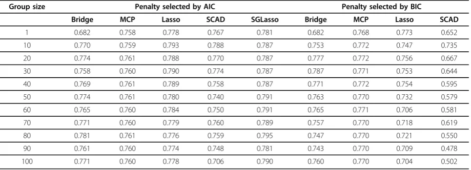
The grouped methods we consider are not well suited to handling overlapping groups by construction. Exten-sions of the grouped methods would thus be needed to efficiently accommodate complications associated with overlapping groups. Existing extensions of the grouped methods designed to solve this type of complication include the overlapping group lasso that allows overlaps between groups of covariates. Some covariates are allowed to occur in more than one group but each time Table 1 Pearson correlation between the true and predicted genomic breeding values for group bridge, MCP, lasso and SCAD for trait T1 based on systematic groups.
Group size Penalty selected by AIC Penalty selected by BIC
Bridge MCP Lasso SCAD SGLasso Bridge MCP Lasso SCAD
1 0.682 0.758 0.778 0.767 0.781 0.682 0.768 0.773 0.652
10 0.770 0.759 0.793 0.788 0.787 0.753 0.772 0.747 0.735
20 0.774 0.761 0.788 0.770 0.787 0.777 0.772 0.756 0.667
30 0.758 0.760 0.790 0.774 0.787 0.787 0.771 0.753 0.644
40 0.769 0.761 0.789 0.758 0.787 0.771 0.772 0.754 0.595
50 0.774 0.761 0.780 0.740 0.791 0.763 0.770 0.732 0.579
60 0.765 0.760 0.784 0.750 0.791 0.765 0.771 0.706 0.581
70 0.771 0.760 0.779 0.760 0.789 0.757 0.770 0.718 0.619
80 0.781 0.761 0.776 0.759 0.795 0.747 0.770 0.721 0.550
90 0.761 0.760 0.774 0.748 0.781 0.743 0.770 0.709 0.478
100 0.771 0.760 0.778 0.706 0.790 0.760 0.770 0.704 0.502
a covariate occurs in one group it gets a new coefficient [34,35]. This makes it possible to select one variable without selecting all the groups containing it. A related extension is the hierarchical (overlapped) group lasso that incorporates both main effects and interactions that obey weak or strong hierarchy (nesting) patterns [36-38]. To check if allowing for overlap among groups indeed improved predictive accuracy, we fitted the hier-archical group lasso model in the glinternet package in R and used10-fold cross-validation to select the optimal
λvalue from a set of 50 values [38]. The estimated pre-dictive accuracies of 0.759, 0.815 and 0.791 for traits 1, 2 and 3, respectively, showed that using overlapping groups did not improve accuracy relative to using non overlapping groups. Other extensions of the grouped methods applicable in slightly different settings include
the group lasso for logistic regression [39], generalized linear models [40] and nonparametric models [41].
Although the performance of the different methods did not differ dramatically for these data the methods often differed with respect to their relative computa-tional efficiencies. Other studies that have compared the performance of the group lasso with other grouped methods, for example, have also found similar results and more. In particular, [24] evaluated the performance of the group lasso relative to group Lars and group non-negative garrote. They found that the group lasso was the slowest of the three group methods because its solution path is not piecewise linear and hence requires intensive computations in large scale problems. The group Lars had comparable performance to the group lasso but was faster because its solution path is piecewise Table 2 Pearson correlation between the true and predicted genomic breeding values for group bridge, MCP, lasso and SCAD for trait T2 based on systematic groups.
Group size Penalty selected by AIC Penalty selected by BIC
Bridge MCP Lasso SCAD SGLasso Bridge MCP Lasso SCAD
1 0.756 0.790 0.826 0.810 0.841 0.828 0.837 0.827 0.795
10 0.779 0.809 0.852 0.840 0.845 0.819 0.839 0.813 0.776
20 0.762 0.809 0.844 0.833 0.845 0.818 0.838 0.779 0.780
30 0.758 0.809 0.836 0.827 0.845 0.801 0.838 0.765 0.744
40 0.710 0.810 0.818 0.788 0.845 0.790 0.838 0.735 0.688
50 0.714 0.809 0.827 0.808 0.846 0.807 0.837 0.746 0.697
60 0.708 0.808 0.810 0.804 0.843 0.810 0.837 0.738 0.708
70 0.700 0.809 0.806 0.804 0.843 0.789 0.837 0.731 0.680
80 0.702 0.809 0.811 0.800 0.844 0.790 0.837 0.735 0.641
90 0.669 0.808 0.795 0.793 0.848 0.785 0.837 0.714 0.607
100 0.704 0.808 0.803 0.792 0.841 0.798 0.837 0.808 0.632
Although listed under AIC, SGLasso used only 10-fold cross validation. The Pearson correlation for ridge regression for comparison is 0.772.
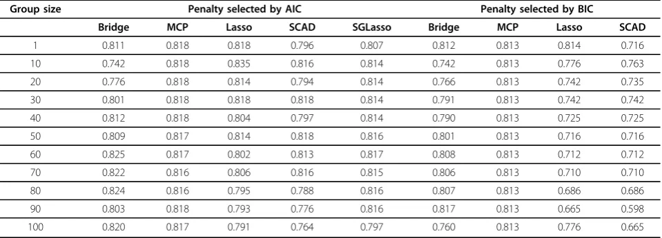
Table 3 Pearson correlation between the true and predicted genomic breeding values for group bridge, MCP, lasso and SCAD for trait T3 based on systematic groups.
Group size Penalty selected by AIC Penalty selected by BIC
Bridge MCP Lasso SCAD SGLasso Bridge MCP Lasso SCAD
1 0.811 0.818 0.818 0.796 0.807 0.812 0.813 0.814 0.716
10 0.742 0.818 0.835 0.816 0.814 0.742 0.813 0.776 0.763
20 0.776 0.818 0.814 0.794 0.814 0.766 0.813 0.742 0.735
30 0.801 0.818 0.818 0.818 0.814 0.791 0.813 0.742 0.742
40 0.812 0.818 0.804 0.797 0.814 0.790 0.813 0.725 0.725
50 0.809 0.817 0.814 0.818 0.816 0.801 0.813 0.716 0.716
60 0.825 0.817 0.802 0.813 0.817 0.808 0.813 0.712 0.712
70 0.822 0.816 0.806 0.816 0.815 0.806 0.813 0.710 0.710
80 0.824 0.816 0.795 0.788 0.816 0.807 0.813 0.686 0.686
90 0.803 0.818 0.793 0.776 0.816 0.817 0.813 0.665 0.598
100 0.820 0.817 0.791 0.764 0.797 0.760 0.813 0.776 0.665
linear [24]. The group non-negative garrote cannot be directly applied to problems in which the total number of covariates exceeds the sample size because it depends explicitly on the full least squares estimates [24].
Conclusions
All the methods produced relatively high estimates of predictive accuracy and hence can be used in genomic prediction research and practice. Systematic grouping or conventional K-means clustering of markers did not lead to any noticeable improvement in predictive accu-racy. The grouped methods may yield better predictions with more sophisticated clustering approaches such as K-means spatial clustering which therefore deserve con-sideration in future studies. Whenever possible, the selection of the penalty parameter for the regularization methods should be done using replicated cross-valida-tion to enhance accuracy of estimates. Nevertheless, selecting the penalty parameter using information theo-retic criteria such as AIC and BIC may occasionally yield better estimates than cross-validation.
List of abbreviations used
SNP: Single Nucleotide Polymorphism; QTL:Quantitative Trait Loci; RSS: Residual Sum of Squares; LASSO: Least Absolute Shrinkage and Selection Operator; MCP: The Minimax Concave Penalty; SCAD: Smoothly clipped absolute deviation; AIC: Akaike Information Criterion, BIC: Schwarz Bayesian Information Criterion.
Competing interests
The authors declare that they have no competing interests.
Authors’contributions
JOO conceived the study, conducted the statistical analysis and drafted the manuscript. HPP read and edited the manuscript and oversaw the project. All the authors read and approved the manuscript.
Acknowledgements
We thank Dr. Torben Schulz-Streeck for useful discussions that helped improve this paper.
Declarations
The German Federal Ministry of Education and Research (BMBF) funded this research and publication within the AgroClustEr“Synbreed - Synergistic plant and animal breeding”(Grant ID: 0315526).
This article has been published as part ofBMC ProceedingsVolume 8 Supplement 5, 2014: Proceedings of the 16th European Workshop on QTL Mapping and Marker Assisted Selection (QTL-MAS). The full contents of the supplement are available online at http://www.biomedcentral.com/bmcproc/ supplements/8/S5
Published: 7 October 2014
References
1. Meuwissen THE, Hayes BJ, Goddard ME:Prediction of total genetic value using genome-wide dense marker maps.Genetics2001,157:1819-1829. 2. Kennard RW:Ridge regression: biased estimation for non-orthogonal
problems.Technometrics1970,12:55-67.
3. Tibshirani R:Regression shrinkage and selection via the lasso.J Roy Statist Soc Ser B1996,58:267-288.
4. Hastie T:Regularization and variable selection via the elastic net.J Roy Statist Soc Ser B2005,67:301-320.
5. Frank IE, Friedman JH:A statistical view of some chemometrics regression tools (with discussion).Technometrics1993,35:109-148. 6. Heslot N, Yang HP, Sorrells ME, Jannink JL:Genomic selection in plant
breeding: a comparison of models.Crop Sci2012,52:146-160. 7. Ogutu JO, Schulz-Streeck T, Piepho H-P:Genomic selection using
regularized linear regression models: ridge regression, lasso, elastic net and their extensions.InBMC Proceedings. Volume 6.BioMed Central Ltd; 2012(Suppl 2).
8. Huang J, Horowitz JL, Ma S:Asymptotic properties of bridge estimators in sparse high-dimensional regression models.Ann Statist2008,36:587-613. 9. Fu WJ:Penalized regressions: The bridge versus the lasso.J Comput
Graph Statist1998,7:397-416.
10. Knight K, Fu W:Asymptotics for Lasso-type estimators.Ann Statist2000,
28:356-1378.
11. Fan J, Li R:Variable selection via nonconcave penalized likelihood and its oracle Properties.J Amer Statist Assoc2001,96:1348-1360.
12. Fan J, Peng H:Nonconcave penalized likelihood with a diverging number of parameters.Ann Stat2004,32:928-961.
13. Whittaker JC, Thompson R, Denham MC:Marker-assisted selection using ridge regression.Genet Res2000,75:249-252.
14. Piepho HP:Ridge regression and extensions for genomewide selection in maize.Crop Sci2009,49:1165-1176.
15. Piepho H-P, Ogutu JO, Schulz-Streeck T, Estaghvirou B, Gordillo A, Technow F:Efficient computation of ridge-regression best linear unbiased prediction in genomic selection in plant breeding.Crop Sci 2012,52:1093-1104.
16. Zhang CH:Nearly unbiased variable selection under minimax concave penalty.Ann Stat2010,38:894-942.
17. Zhang CH:Penalized linear unbiased selection.Department of Statistics and Bioinformatics, Rutgers University; 2007, Technical Report #2007-003. 18. Zhou H:The adaptive lasso and its oracle properties.J Amer Stat Assoc
2006,101:1418-1429.
19. Breheny P, Huang J:Penalized methods for bi-level variable selection.
Stat Interface2009,2:369-380.
20. Breheny P, Huang J:Coordinate descent algorithms for nonconvex penalized regression, with applications to biological feature selection.
Ann Appl Stat2011,5:232-253.
21. Huang J, Breheny P, Ma S:A selective review of group selection in high-dimensional models.Statist Sci2012,27:481-499.
22. Huang J, Ma S, Xie H, Zhang CH:A group bridge approach for variable selection.Biometrika2009,96:339-355.
23. Park C, Yoon YJ:Bridge regression: adaptivity and group selection.J Statist Plann Inference2011,141:3506-3519.
24. Yuan M, Lin Y:Model selection and estimation in regression with grouped variables.J Roy Statist Soc Ser B2006,68:49-67.
25. Simon N, Friedman J, Hastie T, Tibshirani R:A sparse-group lasso.J Comput Graph Statist2013,22:231-245.
26. Nardi Y, Rinaldo A:On the asymptotic properties of the group lasso estimator for linear models.Electron J Statist2008,2:605-633. 27. Wang H, Leng C:A note on adaptive group lasso.Comput Statist Appl
Data Anal2008,52:5277-5286.
28. Zhang C-H, Huang J:The sparsity and bias of the lasso selection in high-dimensional linear regression.Ann Stat2008,36:1567-1594.
29. Peng J, Zhu J, Bergamaschi A, Han W, Noh DY, Pollack JR, Wang P:
Regularized multivariate regression for identifying master predictors with application to integrative genomics study of breast cancer.Ann Appl Stat2010,4:53-77.
30. Friedman J, Hastie T, Tibshirani R:A note on the group lasso and sparse group lasso.2010, arXiv preprint arXiv:1001.0736.
31. Friedman J, Hastie T, Tibshirani R:Regularization paths for generalized linear models viacoordinate descent.2008 [http://www-stat.stanford.edu/ ~hastie/Papers/glmnet.pdf].
32. Yang Y:Can the strengths of AIC and BIC be shared?Biometrika2005,
92:937-950.
33. Martinez JG, Carroll RJ, Müller S, Sampson JN, Chartterjee N:Empirical performance of cross-validation with oracle methods in genomic context.Amer Statist2011,65:223-228.
34. Jacob L, Obozinski G, Vert J-P:Group lasso with overlap and graph lasso.
35. Percival D:Theoretical properties of the overlapping groups lasso.
Electron J Stat2011, 1-21.
36. Zhao P, Rocha G, Yu B:The composite absolute penalties family for grouped and hierarchical variable selection.Ann Stat2009,37:3468-3497. 37. Bien J, Taylor J, Tibshirani R:A lasso for hierarchical interactions.Ann Stat
2013,41:1111-1141, 2013.
38. Lim M, Hastie T:Learning interactions through hierarchical group-lasso regularization.[http://arxiv.org/pdf/1308.2719v1.pdf].
39. Meier L, van der Geer S, Bühlmann P:The group lasso for logistic regression.J Roy Statist Soc Ser B2008,70:53-71.
40. Roth V, Fischer B:The group-lasso for generalized linear models: uniqueness of solutions and efficient algorithms.Proceedings of the 25th annual international conference on machine learningHelsinski, Finland. ICML; 2009, 433-440.
41. Bach F:Consistency of the group lasso and multiple kernel learning.J Mach Learn2008,9:1179-1225.
doi:10.1186/1753-6561-8-S5-S7
Cite this article as:Ogutu and Piepho:Regularized group regression methods for genomic prediction: Bridge, MCP, SCAD, group bridge, group lasso, sparse group lasso, group MCP and group SCAD.BMC Proceedings20148(Suppl 5):S7.
Submit your next manuscript to BioMed Central and take full advantage of:
• Convenient online submission
• Thorough peer review
• No space constraints or color figure charges
• Immediate publication on acceptance
• Inclusion in PubMed, CAS, Scopus and Google Scholar
• Research which is freely available for redistribution