R E S E A R C H
Open Access
A hyperspectral image classification
algorithm based on atrous convolution
Xiaoqing Zhang
1, Yongguo Zheng
1, Weike Liu
2*and Zhiyong Wang
3Abstract
Hyperspectral images not only have high spectral dimension, but the spatial size of datasets containing such kind of images is also small. Aiming at this problem, we design the NG-APC (non-gridding multi-level concatenated Atrous Pyramid Convolution) module based on the combined atrous convolution. By expanding the receptive field of three layers convolution from 7 to 45, the module can obtain a distanced combination of the spectral features of hyperspectral pixels and solve the gridding problem of atrous convolution. In NG-APC module, we construct a 15-layer Deep Convolutional Neural Networks (DCNN) model to classify each hyperspectral pixel. Through the experiments on the Pavia University dataset, the model reaches 97.9% accuracy while the parameter amount is only 0.25 M.
Compared with other CNN algorithms, our method gets the best OA (Over All Accuracy) and Kappa metrics, at the same time, NG-APC module keeps good performance and high efficiency with smaller number of parameters.
Keywords:Deep Convolutional Neural Networks, Hyperspectral image classification, Atrous Convolution, Gridding problem
1 Introduction
Hyperspectral remote sensing is a novel technology that can simultaneously acquire spectral and spatial information at the nanometer scale while maintaining the advantages of the previous wide-band remote sensing technology. Moreover, hyperspectral remote sensing can cover tens or even hun-dreds of continuous narrow-band spectrums formed from chromatic dispersion, such as ultraviolet, visible, near-infrared, and far-infrared bands. Therefore, hyperspectral im-ages (HSI) are often used for fine classification of features [1], such as distinguishing different types of crops or ground ma-terials [2,3]. In recent years, the spatial resolution of hyper-spectral image sensors has been greatly improved. Using AVIRIS sensors, the 20-m resolution of the Indian Pines dataset in 1992 has been improved by the 3.7-m resolution on the Salinas dataset. Then, the reflective optics spectro-graphic imaging system (ROSIS-03) has allowed to further improve to a 1.3-m resolution on the Pavia University data-set. With such an improvement and an abundance of spec-tral features, the number of mixed pixels has been significantly reduced. Hence, the material properties of a
single-pixel have become clearer, enabling to make qualita-tive detection out of small targets more feasible.
Nowadays, HSI classification algorithms are mainly di-vided into two categories: spectral information matching methods and statistical methods. The former methods directly utilize known spectral information in the spec-tral library to identify the types of features in the image. These methods can be used to compare and match the whole band spectral information, or to select some spec-tral bands information of interest, so as to achieve the purpose of classification. Examples of spectral informa-tion matching methods are minimum distance measure [4], binary code matching [5], spectral angle mapping, and spectral information divergence [6]. Such algorithms are mainly used in some HSI processing software, and the application scope and classification accuracy are limited.
Statistical-based classification methods first convert image information into discrete digital matrices and then use strict mathematical derivation algorithms to distin-guish different features. Examples of such methods are
Support Vector Machine (SVM) [7], PCA-based
classifi-cation method [8], and classification methods based on sparse matrix [9]. Statistical-based classification methods usually require the processed data to meet certain
© The Author(s). 2019Open AccessThis article is distributed under the terms of the Creative Commons Attribution 4.0 International License (http://creativecommons.org/licenses/by/4.0/), which permits unrestricted use, distribution, and reproduction in any medium, provided you give appropriate credit to the original author(s) and the source, provide a link to the Creative Commons license, and indicate if changes were made.
* Correspondence:[email protected]
2Center of Information and Network, Shandong University of Science and Technology, Shandong University of Science and Technology, Shandong, China
Full list of author information is available at the end of the article
Zhanget al. EURASIP Journal on Wireless Communications and Networking
(2019) 2019:270
conditions, such as conforming to normal distribution or supporting normalization. Thus, the high requirement of the digital matrices and the previous data processing will inevitably reduce the accuracy of classification.
In recent years, many researchers have used Convo-lutional Neural Networks (CNN) to classify hyper-spectral images and achieved good results. CNN learn the feature maps of samples through convolution and down-sampling hierarchical operations. Through mul-tiple feedback optimizations, it automatically learns and finally obtains hierarchical features. In particular,
CNNs have developed towards the direction of “deep”
and many classic architectures. For instance, AlexNet
[10] VGG16, GoogleNet [11], and ResNet [12] can
achieve good results in target recognition and classifi-cation on huge datasets. Usually, those datasets (e.g., ImageNet, PASCAL VOC) are composed of tens of thousands of samples, i.e., the spatial features of three dimension (RGB) images. These Deep Convolutional Neural Networks (DCNN) deepen with the increase of parameters and computation; thus, the training
process becomes more difficult [13–15]. Therefore,
how to construct a lightweight model has become a hot research topic. To achieve this goal, models such as MobileNets [16], Squeezenet [17], Xception [18],
and others [19, 20] use deep-wise separable
convolu-tion or dilated convoluconvolu-tion instead of full convoluconvolu-tion to make them lightweight and effective.
Since HSI is different from an RGB image, the classical DCNN model cannot be directly applied to HSI classifi-cation. Indeed, such a classification raises three main problems:
a) Multiple spectral features. HSI has hundreds of dimensions of spectral features. If directly input DCNN model, the kernels of each layer should have several times the number of dimensions of the original, which causes the number of parameters to increase exponentially. This phenomenon is called dimension disaster. Moreover, a further
dimensional reduction reduces accuracy, such as SVM [7].
b) Small spatial size of hyperspectra dataset. Usually, the HSI dataset has little spatial information, even only a picture of tens of thousands of pixels. This could be not enough for a DCNN model to achieve effectively classification by extracting spatial features, and it is easy to cause overfitting.
Therefore, the common hyperspectral CNN model [21,22] has only two convolution layers; thus, it is difficult to learn the combination features over a long distance.
c) The number of parameters has to be kept as small as possible to achieve fast computational speed.
This is necessary because in the future, it
envisioned the possibility to run a DCNN model on mobile devices and provide real-time feedback. For example, real-time land information can be pro-vided to farmers through HIS.
To solve the above three problems, in this paper, we combine the atrous pyramid convolution to obtain HSI’s spectral features more effectively by solving the gridding problem in the atrous convolution. We acquire the fea-ture maps of the spectral information in all dimensions and replace the fully connected layer with two convolu-tional layers. It significantly reduces the number of pa-rameters and provides as output the material label of a single hyperspectral pixel.
The rest of this paper is organized as follows. In Sec-tion 2, we introduce the atrous convoluSec-tion. SecSec-tion 3 briefly introduces gridding and non-gridding problems. Section 4 gives the algorithm of NG-APC module. In Section 5, we experimentally compare the performance of our method with SVM and some other CNN-based algorithms. Section 6 draws some conclusions.
2 Atrous convolution analysis
In the field of image semantic segmentation, Chen
proposed the Deeplab model [23] in 2014, which
in-troduced the atrous convolution. In 2017, Chen
pro-posed the atrous spatial pyramid pooling [24] [25],
which was applied to the up-sampling part of the encode-decode architecture to expand the convolution receptive field to acquire long-distance features effect-ively. It performed good in RGB image semantic segmentation. The core idea is to expand the recep-tive field of different scales by changing the size of the atrous while maintaining the size of the convolu-tion kernel and to quickly obtain a larger range of feature maps.
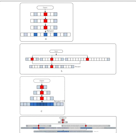
As shown in Fig. 1, each small square represents a pixel. The red pixel is the center pixel of the convolu-tion; the blue pixels are associated with the center pixel and covered by the atrous convolution. That is to say, the feature of blue pixels can be sampled at that
location. The gray ones are the holes from which the convolution cannot learn the feature of the location. Through one layer of atrous convolution, it is possible to associate far apart features, that is, to obtain a com-bined feature of a longer distance dimension.
Fig. 1Atrous convolutions sketch map.a1D atrous convolutions with kernel, dilation rate is 1, 2, and 4;b2D atrous convolutions with kernel, dilation rate is 1, 2, and 4; atrous convolutions enlarge the receptive field while keeping the same kernel size
The 1D reception field equation is as follows:
F1¼ðk−1Þ rþ1 ð2Þ
whereF1is the 1D reception field,kis the size of the convolution kernel,ris the rate, and the size of hole isr
−1. For instance, in the case of kernel = 3, rate = 4, we can getF1= 9. In the case of 2D convolution, the recep-tion field is Eq. (3):
F2¼ F12 ð3Þ
There are three ways to get the same receptive field, if we use the standard convolution. First, using the big ker-nel of 7, the parameters are also expanded by 7/3 times; Second, using the four-layer convolution structure ker-nel of 3, the parameters are expanded by 4 times; Third, using two-layer convolution kernel of 3, the connection is expanded by max pooling or average pooling in the middle, and the parameter quantity is expanded by 2 times. However, the boundary is blurred, details are lost, and errors are introduced when pooling. It can be seen that the atrous convolution has great advantages in expanding the receptive field. At the same time, it also exists as the problem of not learning all features, which is called gridding problems.
3 Gridding and non-gridding problems
Atrous convolutions with dilation rates larger than the one will generate holes called gridding artifacts, 2D atrous convolution with 3 × 3 kernel, and a dilation rate ofr= 4 has a 9 × 9 receptive field. However, the number of points that are actually involved in the computation is only 9 out of 81, which implies that the actual receptive field is still 3 × 3 see Fig.1b.
If we use the atrous convolution at the same rate or multiplying rate, gridding and non-gridding prob-lems will become worse. For example, if the rate is 2, 2, and 2 or 2, 4, and 8, this problem will show up
[26]. In Fig. 2, the atrous convolution of different
atrous rates is selected to convolute from top to bot-tom. The red pixel in the figure is the central pixel of the convolution kernel, which is combined with the features of other locations by different atrous rate to construct a feature map, regardless of the size of rate and the number of convolution layers. According to the principle of convolution, although the data of other positions will be introduced after the convolu-tion, the data of the center position (red) will always exist. Blue pixels are positions where features can be obtained by atrous convolution and the more the number of combinations. The higher redundancy, the deeper of the blue color.
Gridding and non-gridding sketch map is shown in Fig. 2. It can be seen from Fig. 2a, after three-layer
atrous convolution where atrous rate is set to 3, the re-ception field can be expanded to 12. But the effective connection point is 5, and the adjacent points of the red pixels are not connected.
In this case, the efficiency of the receptive field (ERF) is 5/12, and the gridding problem is obvious. Since the convolution kernel has holes, after several superimposed atrous convolutions, there will be a problem that the fea-tures of the data in the receptive field are incomplete. Hence, it is also the essential cause of the gridding prob-lem. For the gridding problem, the researchers have pro-posed two solutions:
First is the parallel method, in which we use differ-ent rates in the same layer of convolution and then concatenate the results of the convolution. Chen used the parallel atrous convolution with the rate = 6, 12, 18, and 24 in DeepLabv2. It groups several dilated convolutional layers and applies dilation rates without a common factor relationship. ASPP (Atrous Spatial
Pyramid Pooling) improved encoding part and
achieved a better semantic segmentation performance. Sachin Mehta improved the Resnet architecture in the
efficient spatial pyramid (ESP) module [24], using
atrous convolution rate = 2, 4, 8, and 16 to obtain feature maps of different receptive fields, and then concat to get the final feature maps by reusing the ESP structure. It achieved better recognition and seg-mentation results in the urban street scene of the
PASCAL VOC dataset. Figure 2b illustrates the first
approach and concatenates the result of the convolu-tion with three branches, which atrous rate = 2, 4, and 8 on the input data. Receptive field is 17, and the ERF is 7/17, which improved the gridding prob-lem. This approach is similar to inception, which widens DCNN and concatenates multiple branches with different size of kernel. The receptive field is 17/ 3 times that of a standard convolution of 3 kernel. Through only one layer of convolution, the reception field is enlarged and the parameter quantity is not in-creased. However, there is still a gridding problem in this approach. If you want to achieve non-gridding, you need to use a continuous atrous rate. It is equivalent to a large kernel, but it loses the advantage of small convolution kernel with fewer parameters.
Second, as is shown in Fig. 2c, we call it the serial method. It used different atrous rate concatenated multi-layer convolution, by controlling the size of the
rate to de-gridding. In 2018, Wang [27] proposed
After using the rate = 1, 2, and 3 atrous convolution layers, the receptive fieldF1= 13 and the ERF = 1, which is two times of the standard three-layer concatenated convolution of 3 kernels andF1= 7. Therefore, all the features in the receptive field are obtained. We call this kind of scenario as non-gridding.
Under the condition of non-gridding, the calculation of rate and reception field in serial mode is obtained by formulas (4) and (5):
Fd¼ Fd−1þ2rd ð4Þ
fr1 maxrdmax¼¼1F;dF1 max−1 ¼3;F1¼3 Fdmax¼ Fd−1þ2rdmax
ð5Þ
where r is atrous rate, d is the number of layers in the serial convolution, max is the maximum value that can be obtained at non-gridding,Fis receptive field, and the Fig. 2Gridding and non-gridding sketch map.aAtrous convolution cascade of three layers of the same size rate.bThree atrous convolution stitching of rate = 2, 4, and 8.cThree-layer rate = 1, 2, and 3 atrous convolution cascade.dThree-layer atrous convolution cascade after splicing of 1, 3, and 9 and 1, 3, and 18
calculation of the first layer of convolutionFcan be got-ten in formula (2). In this paper, we only discuss and analyze the case of 1D convolution and of 3 kernels.
In summary, both of these two methods can improve the efficiency of convolution, expand the reception, and reduce the gridding problem.
4 NG-APC module
In this paper, combining these two methods of solving the gridding problem and introducing inception model, we propose a non-gridding multi-level concatenated atrous pyramid convolution module (APC). NG-APC module is divided into two parts. The first part is atrous pyramid convolution, while the second part is di-vided into several branches. Each branch uses a different atrous rate convolution and then merges together, which can achieve the maximum reception field of the non-gridding atrous convolution.
In the first part of NG-APC module, the convolution
depth is n, atrous pyramid convolution depth isn−1.
Formula (5) gives the desirable maximum value of atrous rate under non-gridding conditions, which can be re-duced according to the actual situation.
Layer n of NG-APC module is the second part of
model. It is a convolution layer composed of multiple branches. The number of branches can be set, according to the requirement of receptive field in practical applica-tion. The rate of each branch is according to formula (6):
of the module, d denotes the layer of the convolution,
and max denotes the maximum value of rand F in the
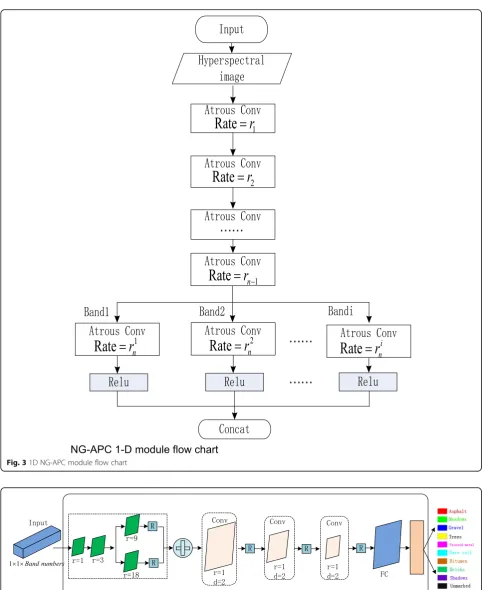
non-gridding condition.1D NG-APC module flow chart
is shown in Fig.3.
In Fig. 3, n is the number of convolution layers, and the default value is 3, which can be modified. The num-ber of branches of the module isi, and ri
n is atrous rate. According to formulas (5) and (6), ri
nis not greater than
ri
nmax, and Fin is reception field, which can obtain the global farthest distance feature. Figure2d is an example of NG-APC module, which has three convolution layers. The first layer atrous rate is 1, the second layer atrous rate is 3, and the third layer has two branches. The atrous rate of branch 1 is 9 and reception field is 27. The atrous rate of branch 2 is 18 and reception field is 45. The holes in branch 2 can be filled by branch 1, so the whole is non-gridding atrous pyramid.
In summary, it can accurately mark the category of each pixel, by using the atrous convolution to collect features between dimensions with large span and
construct an appropriate deep learning architecture to learn the spectral features, for the spectral dimension of 100~200 of each pixel. In the classification of hyperspec-tral image, atrous convolution is effective in replacing traditional convolution in DCNN. Based on the non-gridding atrous pyramid convolution, this paper designs a light weight depth learning architecture model for spectral information classification of hyperspectral im-ages. The hyperspectral image NG-APC classification architecture model is divided into four parts.
a) Input the pixels as a single hyperspectral image, 1 × 1 × band numbers;
b) Input the pixels into the NG-APC module, where the number of convolution layersN= 3, the num-ber of branchesI= 2, the convolution of 128 kernel, the activation function uses ReLu, then the use con-cat function to integrate the feature map together to become the feature map of band numbers × 256. c) Perform three-layer 1D convolution on the feature
map while stride = 2. The number of convolution kernel is halved for every convolution layer and fi-nally get a (band numbers/8) × 32 feature map.
Output the classification results, through the fully con-nected (FC) layer and the Softmax layer. As is shown in Fig.4:
5 Experimental results and discussion
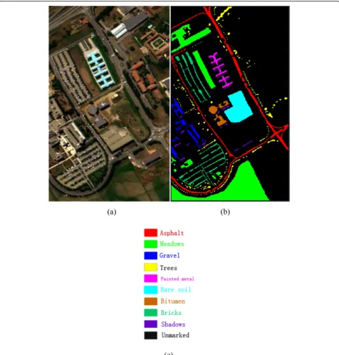
The goal of this algorithm is to obtain the material prop-erties of a single-pixel for the identification of different kinds of ground objects in hyperspectral images. In the three public available hyperspectral datasets [26–31], the Indian Pines datasets and Salinas datasets target the farmland of different crops and the natural topography. They are continuous large areas of the same category, and the classification effect will be better by using the method of spatial spectrum combination. Since our algo-rithm aims at small target recognition of different fea-tures, we select the Pavia University dataset to verify the effectiveness of the algorithm. This dataset is one of the common scenes in the city, which is in line with the goal of this algorithm.
5.1 Experimental dataset
Pavia University dataset (as shown in Fig.5) is from Ger-many’s Reflective Optics Spectrographic Imaging System (ROSIS-03) in 2003.
It is a part of the hyperspectral data of the image of Pavia, Italy, with a spatial resolution of 1.3 m. The data-set has a total of 610 × 340 pixels. The spectral image
resamples 115 samples in the 0.43–0.86 μm wavelength
Fig. 31D NG-APC module flow chart
Fig. 4Hyperspectral image NG-APC classification architecture model diagram
Fig. 5Pavia University dataset images.aFalse-color composite.bGround truth. Land cover classes, black area represents unlabeled pixels
42776 labeled pixels and 9 labeled samples, as is shown in Table1.
In the dataset, when we randomly select the similar la-beled pixels in different spatial locations, the features of shadows and painted metal are more consistent. How-ever, the spectral features of bitumen, Gravel, etc., are quite different. During the experiment, we randomly div-ide the labeled samples into training sets and test sets according to the ratio of 80% and 20%. The unlabeled sample pixels are background pixels. Actually, there should be different material labels. Because they are not labeled, they are not used for training. Otherwise, it will affect the accuracy of the identification classification.
Figure 5 shows the false color composite image and
ground truth with different land cover classes.
5.2 Results and discussion
We set the experiment parameters as follows: learning rate is 0.9, the activation function is Relu, batch is 100, and the optimization strategy uses SGD. The model train and test are on a single NVIDIA GTX 980 4 GB GPUs and with 8 G memory.
In this paper, we compare NG-APC model with the classical SVM, the new 1D-CNN [28, 29] 2D-CNN [30],
3D-CNN algorithms [31–34], and RNN [35]. We refer
some of these algorithms by nshaud/DeepHyperX on GitHub. We set training sample 80%, test sample 20%, and keep some default parameter settings, such as patch size is 7 and epoch is 50.
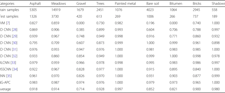
In Table2, we compare the classification results of the proposed NG-APC with other classification algorithms (SVM, 1D CNN, 2D CNN, 3D CNN, and RNN). NG-APC module belongs to 1D CNN. The classification re-sults of NG-APC algorithm are better than the 1D and 2D CNN classification methods in gravel, meadows, and
bitumen feature classification. Even though NG-APC al-gorithm has less accuracy than 3D CNN [32] classifica-tion results in bitumen and bricks features, it has much higher than the average level (0.821 and 0.900).
Table 3 shows confusion matrices for the Pavia
Uni-versity dataset. It can be seen from the detailed classifi-cation accuracy of all the classes, which is calculated from one arbitrary train/test partition. The cell of ith
row and jth column means the probability that the ith
class samples is classified as the jthclass. The percent-ages on diagonal line are just the classification accuracy of corresponding class. The proposed algorithm
per-forms under 95% in only two classes (bitumen and
bricks) among the nine classes. These two class samples are wrongly classified as asphalt with 3.38% and 3.26% separately. As shown in the Table 1, the two classes are the ones with smaller numbers of samples. The more similar two classes of spectral domain, the higher prob-ability they are wrongly classified to each other.
5.3 The accuracy assessment criteria for classification
We use OA (overall accuracy) and Kappa (Kappa coeffi-cient) as the criteria for classification of HSI. OA refers to the proportion of correctly classified samples to all classified samples. The formula is as follows (7):
OA¼ PK
i¼1C ið Þ;i
M ð7Þ
whereM is the total sample number of one class,Kis
the number of categories, andC(i,i) is the current classi-fied sample by the algorithm.
Kappa is used to calculate the similarity between the classification results of ground and the real distribution
Table 2Classification results of different categories by various methods
Categories Asphalt Meadows Gravel Trees Painted metal Bare soil Bitumen Bricks Shadows
Train samples 5305 14919 1679 2451 1076 4023 1064 2945 558
Test samples 1326 3730 420 613 269 1006 266 737 189
SVM [7] 0.827 0.859 0.000 0.730 0.982 0.196 0.000 0.740 1.000
1D CNN [28] 0.869 0.906 0.385 0.899 0.993 0.604 0.706 0.788 0.997
1D CNN [29] 0.939 0.967 0.748 0.949 0.998 0.916 0.771 0.860 0.932
2D CNN [30] 0.795 0.709 0.607 0.873 0.999 1.000 0.999 0.961 0.898
3D CNN [31] 0.976 0.955 0.947 0.976 1.000 0.981 0.983 0.985 1.000
3D CNN [32] 0.933 0.860 0.854 0.949 1.000 0.999 1.000 0.998 0.978
DLCNN [33] 0.979 0.959 0.966 0.978 0.998 0.995 0.983 0.986 0.997
DSSCNN [34] 0.922 0.967 0.828 0.977 1.000 0.915 0.895 0.840 1.000
RNN [35] 0.961 0.970 0.826 0.970 1.000 0.931 0.903 0.877 0.999
NG-APC 0.983 0.987 0.974 0.976 1.000 0.979 0.973 0.965 1.000
Average 0.918 0.914 0.714 0.928 0.997 0.852 0.821 0.900 0.980
of ground objects with disperse analysis method, the for-mula is as follows (8):
Kappa¼M ground object is divided into a particular category,C(+,
i) is the total number of pixels, in which the ground ob-ject actually belongs to a particular category.
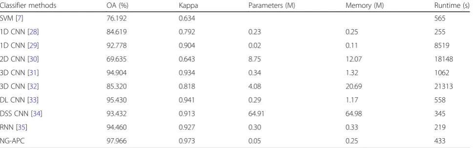
In Table 4, we compare five metrics (i.e., OA, Kappa, the parameters quantities, memory usage, and the run-time) with the other approaches. Compared with the 1D CNN models, whose parameters and runtime are equiva-lent, the NG-APC model gets better results on OA and Kappa. OA increases from 84.619% and 92.778% to 97.966%, while Kappa increases from 0.792 and 0.904 to
0.973. When comparing with the best 3D CNN [33],
whose number of parameters and memory are 5.8 times and 4.68 times larger than NG-APC model. At the same time, OA of NG-APC increases 2.54% and Kappa of NG-APC increases 0.032, respectively. Therefore, the NG-APC model is the best one in those convolution models. It not only has high accuracy classification
results, but also has smaller parameters and faster runtime.
6 Conclusions
In this paper, we propose a 15-layer DCNN model with NG-APC module to classify single-pixel of HSI. This model has solved three problems in HSI classification. First, the single-pixel classification of HSI learns the whole spectral information of each pixel, which not only solves the prob-lem of large computational complexity of high-dimensional data, but also solves the problem of insufficient samples in DCNN training. Second, aiming at the reasonable combin-ation of 1D atrous convolution, we propose NG-APC mod-ule, which solves the gridding problem and enlarges the receptive field from 7 to 45. Moreover, the classification ac-curacy is improved by learning the long-distance feature combination. The OA reaches 98% and the Kappa reaches 0.974 on the Pavia University dataset, whose are superior to many kinds of 1D, 2D, and 3D CNN models. Third, re-placing the 1D convolution with the full connection layer, although the model is a 15-layer DCNN, the parameters are similar to those of the same type of 1D-CNN of five layers, which meets the requirements of small parameter models. In conclusion, NG-APC model is an excellent DCNN model for HSI classification.
Table 3The detailed classification accuracies of all the categories for Pavia University with NG-APC model
Asphalt (%) Meadows (%) Gravel (%) Trees (%) Painted metal (%) Bare soil (%) Bitumen (%) Bricks (%) Shadows (%)
Asphalt 99.17 0.00 0.60 0.00 0.00 0.08 0.00 0.15 0.00
Meadows 0.00 98.23 0.00 0.16 0.00 1.61 0.00 0.00 0.00
Gravel 0.24 0.00 97.62 0.00 0.00 0.00 0.00 2.14 0.00
Trees 0.00 2.77 0.00 96.74 0.00 0.33 0.00 0.16 0.00
Sheets 0.00 0.00 0.00 0.00 100 0.00 0.00 0.00 0.00
Bare soil 0.00 1.19 0.00 0.30 0.00 98.51 0.00 0.00 0.00
Bitumen 3.38 0.00 0.00 0.00 0.00 1.88 94.74 0.00 0.00
Bricks 3.26 0.14 0.54 0.00 0.00 1.22 0.00 94.84 0.00
Shadows 0.00 0.00 0.00 0.00 0.00 0.00 0.00 0.00 100
Table 4Classification results obtained by different approaches on Pavia University dataset
Classifier methods OA (%) Kappa Parameters (M) Memory (M) Runtime (s)
SVM [7] 76.192 0.634 565
Abbreviations
AA:Averaged accuracy; CNN: Convolutional neural networks; DCNN: Deep convolutional neural networks; FC: Fully connected layer; HSI: Hyperspectral images; NG-APC: Non-gridding multi-level concatenated atrous pyramid con-volution; OA: Over all accuracy
Acknowledgements
Thanks for the support of the National Virtual Simulation Laboratory Center for Coal Mine Safety Mining, Shandong University of Science and Technology.
Authors’contributions
All authors contribute to the concept, the design, and developments of the algorithm and the simulation results in this manuscript. All authors read and approved the final manuscript.
Funding
This project was supported by foundation of the National Natural Science Fund (41876202, 41774002, 61976126) and Natural Science Foundation of Shandong Province (ZR2017MD020).
Availability of data and materials
The authors declare that all the data and materials in this manuscript are available from the author.
Competing interests
The authors declare that they have no competing interests.
Author details
1College of Computer Science and Engineering, Shandong University of Science and Technology, Shandong, China.2Center of Information and Network, Shandong University of Science and Technology, Shandong University of Science and Technology, Shandong, China.3College of Geomatics, Shandong University of Science and Technology, Shandong, China.
Received: 20 September 2019 Accepted: 31 October 2019
References
1. Q.X. Tong, B. Zhang, L.F. Zheng, inTechnology and Application. Hyperspectral remote sensing principle (Higher Education Press, Beijing, 2006), pp. 1–2
2. R.R. Nidamanuri, B. Zbell, Transferring spectral libraries of canopy reflectance for crop classification using hyperspectral remote sensing data. Biosystems Engineering110(3), 231–246 (2011).https://doi.org/10.1016/j.biosystemseng. 2011.07.002
3. U. Seiffert, F. Bollenbeck, H.P. Mock, et al, Clustering of crop phenotypes by means of hyperspectral signatures using artificial neural networks. Hyperspectral Image and Signal Processing: Evolution in Remote Sensing (WHISPERS), in: 2010 2nd Workshop on, IEEE, 1-4 (2010).https://doi.org/10. 1109/WHISPERS.2010.5594947
4. C.I. Chang, An information-theoretic approach to spectral variability, similarity, and discrimination for hyperspectral image analysis. IEEE Trans. Inf. Theory46(5), 1927–1932 (2000).https://doi.org/10.1109/18.857802 5. X. Jia, J.A. Richards, Binary coding of imaging spectrometer data for fast
spectral matching and classification. Remote Sensing Environ.43(1), 47–53 (1993).https://doi.org/10.1016/0034-4257(93) 90063-4
6. F.A. Kruse, A.B. Lefkoff, J.W. Boardman, The spectral image processing system (SIPS)-interactive visualization and analysis of imaging spectrometer data. Remote Sensing Environ.44(2), 145–163 (1993).https://doi.org/10. 1063/1.44433
7. S.Madan, C.Pranjali, in International conference on computing Communication Control & Automation. A review of machine learning techniques using decision tree and support vector machine. (IEEE ICCUBEA 2017), pp.1-7.https://doi.org/10.1109/ICCUBEA.2016.7860040
8. M.B. Luis, F. Olac, Object detection using image reconstruction with PCA. Image Vis. Comput.27, 2–9 (2009).https://doi.org/10.1016/j.imavis. 2007.03.004
9. L.P. Zhou, L. Wang, P. Ogunbona, Discriminative sparse inverse covariance matrix: application in brain functional network classification. CVPR, 1–8 (2014).https://doi.org/10.1109/CVPR.2014.396
10. J. Sun, X. Cai, F. Sun, Scene image classification method based on Alex-Net model. ICCSS, 363–367 (2016).https://doi.org/10.1109/ICCSS.2016.7586482 11. C.Szegedy, V.Vanhoucke, Rethinking the inception architecture for computer
vision. arXiv:1512.00567v3[cs.CV],1-10(2015)
12. S.Christian, I.Sergey, V. Vincent, Inception-v4, Inception-ResNet and the impact of residual connections on learning. arXiv: 1602.07261 v2 [cs.CV], 1-12(2016)
13. C.H. Chen, A cell probe-based method for vehicle speed estimation, IEICE Transactions on Fundamentals of Electronics. Communications and Computer Sciences, E103-A(1), 2020.
14. C.H. Chen, F.J. Hwang, H.Y. Kung, Travel time prediction system based on data clustering for waste collection vehicles. IEICE Trans. Inf. Syst.E102-D(7), 1374–1383 (2019)
15. C.H. Chen, An arrival time prediction method for bus system. IEEE Internet of Things Journal5(5), 4231–4232 (2018).https://doi.org/10.1109/JIOT.2018. 2863555
16. A.G.Howard, M.L.Zhu, B.Chen, MobileNets: efficient convolutional neural networks for mobile vision applications. arXiv: 1704. 04861v1 [cs.CV],1-9(2017).
17. Landola NN, S Han, M Moskewicz, SqueezeNet: Alexnet-level accuracy with 50x fewer parameters and < 0.5 Mb model size. arXiv preprint arXiv:1602. 07360, 1-13(2016).
18. F.Chollet, Xception: deep learning with depthwise separable convolutions. arXiv: 1610.02357v3 [cs.CV], 1-8(2017).
19. J.S. Pan, L. Kong, T.W. Sung, P.W. Tsai, V. Snasel,α-Fraction first strategy for hierarchical wireless sensor networks. J. Internet Technol.19(6), 1717–1726 (2018)
20. J.S. Pan, C.Y. Lee, A. Sghaier, M. Zeghid, J. Xie, Novel systolization of subquadratic space complexity multipliers based on Toeplitz matrix–vector product approach. IEEE Trans. Very Large Scale Integration Syst.27(7), 1614– 1622 (2019)
21. B. Cui, X.Y. Xie, X. Ma, G. Ren, Y. Ma, Super pixel-based extended random walker for hyperspectral image classification. IEEE Trans. Geoscience Remote Sensing56(6), 3233–3243 (2018)
22. B. Cui, X.Y. Xie, S. Hao, J. Cui, Y. Lu, Semi-supervised classification of hyperspectral images based on extended label propagation and rolling guidance filtering. Remote Sensing10(4), 515 (2018)
23. L.C.Chen, P.George, K.Iasonas, M.Kevin, L.Y.Alan, Semantic image
segmentation with deep convolutional nets and fully connected CRFs. ICLR arXiv: 1412.7062[cs.CV], 1-14 (2014).
24. L.C.Chen, P.George, DeepLab: semantic image segmentation with deep convolutional nets, atrous convolution, and fully connected CRFs. arXiv: 1606.00915v2 [cs.CV],1-14( 2017).
25. L.C.Chen, P.George, S.Florian, A.Hartwig, Rethinking atrous convolution for semantic image segmentation. arXiv:1706.05587v3[cs.CV], 1-10 ( 2017). 26. S.Mehta, M.Rastegari, A.Caspi, ESPNet: efficient spatial pyramid of dilated
convolutions for semantic segmentation. arXiv:1803.06815v3[cs.CV],1-29(2018).
27. P.Wang, P.F.Chen, Y.Yuan, Understanding convolution for semantic segmentation. arXiv:1702.08502v3[cs.CV], 1-10(2018).
28. W. Hu, Y. Huang, W. Li, Deep convolutional neural networks for
hyperspectral image classification. J. Sensors, 1–12 (2015).https://doi.org/10. 1155/2015/258619
29. A.Boulch, N.Audebert, D. Dubucq, Auto encodeurs pour la visualisation d'images hyperspectrales. GRETSI, 1-4(2017).
30. V.Sharma, A.Diba, T.Tuytelaars, L.Van, Hyperspectral CNN for image classification & band selection, with application to face recognition. Technical Report, 1-14(2016).
31. M.Y. He, B. Li, H.H. Chen, Multi-scale 3D deep convolutional neural network for hyperspectral image classification. ICIP, 3904–3908 (2017).https://doi. org/10.1109/ICIP.2017.8297014
32. Y.S. Chen, H.L. Jiang, C.Y. Li, Deep feature extraction and classification of hyperspectral images based on convolutional neural networks. IEEE Trans. Geoscience Remote Sensing54(10), 6232–6251 (2016).https://doi.org/10. 1109/TGRS.2016.2584107
33. A.B. Hamida, A. Benoit, P. Lambert, 3-D deep learning approach for remote sensing image classification. IEEE Trans. Geosciences Remote Sensing56(8), 4420–4434 (2018)
34. W.J.Wang, S.G.Dou, Z.M.Jiang, A fast dense spectral–spatial convolution network framework for hyperspectral images classification. Remote Sensing,1-19(2018).
35. L. Mou, P. Ghamisi, X.X. Zhu, Deep recurrent neural networks for hyperspectral image classification. IEEE Trans. Geoscience Remote Sensing
55(7), 3639–3655 (2017).https://doi.org/10.1109/TGRS.2016.2636241
Publisher’s Note