A 3 D electrical resistivity model beneath the focal zone of the 2008 Iwate Miyagi Nairiku earthquake (M 7 2)

L E T T E R

Open Access

A 3-D electrical resistivity model beneath the

focal zone of the 2008 Iwate-Miyagi Nairiku

earthquake (M 7.2)

Hiroshi Ichihara

, Shin'ya Sakanaka

, Masaaki Mishina

, Makoto Uyeshima

, Tadashi Nishitani

, Yasuo Ogawa

,

Yusuke Yamaya

, Toru Mogi

, Kazuhiro Amita

and Takuya Miura

Abstract

The 2008 Iwate-Miyagi Nairiku earthquake (M 7.2) was a shallow inland earthquake that occurred in the volcanic front of the northeastern Japan arc. To understand why the earthquake occurred beneath an active volcanic area, in which ductile crust generally impedes fault rupture, we conducted magnetotelluric surveys at 14 stations around the epicentral area 2 months after the earthquake. Based on 56 sets of magnetotelluric impedances measured by the present and previous surveys, we estimated the three-dimensional (3-D) electrical resistivity distribution. The inverted 3-D resistivity model showed a shallow conductive zone beneath the Kitakami Lowland and a few conductive patches beneath active volcanic areas. The shallow conductive zone is interpreted as Tertiary sedimentary rocks. The deeper conductive patches probably relate to volcanic activities and possibly indicate high-temperature anomalies. Aftershocks were distributed mainly in the resistive zone, interpreted as a brittle zone, and not in these conductive areas, interpreted as ductile zones. The size of the brittle zone seems large enough for a fault rupture area capable of generating an M 7-class earthquake, despite the areas distributed among the ductile zones. This interpretation implies that 3-D elastic heterogeneity, due to regional geology and volcanic activities, controls the size of the fault rupture zone. Additionally, the elastic heterogeneities could result in local stress concentration around the earthquake area and cause faulting.

Keywords:Magnetotelluric; Iwate-Miyagi earthquake; 3-D resistivity; Inland earthquake

Findings Introduction

The 2008 Iwate-Miyagi Nairiku earthquake (M 7.2) was an inland earthquake that occurred in the vicinity of the volcanic front of the northeastern Japan arc on 14 July 2008. The focal mechanism of the earthquake was a re-verse type, which is consistent with the crustal deform-ation displaying east–west contraction around the study area (Miura et al. 2002, 2004). Aftershocks of the earth-quake were distributed within an area of 50 × 15 km and showed a complex distribution (Figure 1) (Okada et al. 2012). A curious feature of the earthquake was that

volcanic areas (Mt. Kurikoma, Mt. Yakeishi, and Onikobe Caldera) surrounded the earthquake area. In general, duc-tile areas caused by high temperature and partial melting are distributed beneath volcanic regions. Because these ductile areas impede the propagation of fault ruptures, it would seem difficult for large earthquakes to occur in volcanic regions. To address this question and better understand the relationships between inland earthquakes and volcanic activity, detailed structural investigations are required.

The magnetotelluric (MT) method reveals the distribu-tion of electrical resistivity and has been used to clarify the geology, high-temperature anomalies, and fluid distri-bution around earthquake zones (e.g., Mitsuhata et al. 2001; Ogawa et al. 2001; Sarma et al. 2004; Unsworth and Bedrosian, 2004; Ichihara et al. 2008, 2009, 2011; Wannamaker et al. 2009; Yoshimura et al. 2009). Mishina (2009) conducted MT surveys along three survey lines * Correspondence:h-ichi@jamstec.go.jp

1

Research and Development Center for Earthquake and Tsunami, Japan Agency for Marine-Earth Science and Technology, Yokosuka 237-0061, Japan 2

Earthquake Research Institute, The University of Tokyo, Tokyo 113-0032, Japan

Full list of author information is available at the end of the article

across the northern edge, central part, and southern edge of the aftershock area (Figure 1) and estimated resistivity distributions based on two-dimensional (2-D) inversions. The models showed low-resistivity anomalies around the earthquake area that imply crustal fluid flows. They also showed significant differences among the resistivity profiles, which indicate strong three-dimensionality. However, 2-D in-version of a strong three-dimensional (3-D) resistivity struc-ture often results in inaccurate models (e.g., Siripunvaraporn et al. 2005b). Additionally, MT data were not measured around the epicenter of the main shock. In this study, we conducted wide-band MT measurements around the epi-central area and updated the resistivity models based on a 3-D inversion. Then, we interpreted the geological and thermal heterogeneity based on the estimated resistivity model and discussed the relationship between the earth-quake and these heterogeneities.

Magnetotelluric measurements and impedances

Wide-band MT surveys were conducted at 14 sites along a profile passing through the epicenter of the earthquake in August 2008 (Figure 1). We recorded two horizontal components of electric field and three components of mag-netic field using MTU2000 systems (Phoenix Geophysics, Ltd., Toronto, Canada). The electric and magnetic fields

were measured using Pb-PbCl2 electrodes and induction

coils, respectively. The recorded time series were converted into frequency-domain MT impedance tensors between 320 and 0.00034 Hz by using the SSMT200 system

(Phoenix Geophysics, Ltd.). The remote reference tech-nique (Gamble et al. 1979) was applied in the estimation of MT impedances using horizontal magnetic field data from Sawauchi station (Figure 1), which yielded high-quality MT responses.

We then evaluated the dimensionality of the resistivity distribution based on MT impedances and geomagnetic transfer functions at 56 sites: 14 sites evaluated by this study, 41 sites by Mishina (2009), and 1 site by the Geo-graphical Survey Institute. Figure 2 shows the phase tensor ellipses (Caldwell et al. 2004) and Parkinson's

in-duction vectors (Parkinson 1962). The azimuths of Φmax

(α−β) in the phase-tensor ellipses were directed do-minantly toward 115° to 295° in the long period (227 s in Figure 2). This azimuth is perpendicular to the strike azi-muth of the NE Japan arc. On the other hand, no obvious trend was found from the phase tensor in the shorter period or the induction vectors in all periods (Figure 2). Additionally, large |β| values (>10°) were recognized in more than half of the phase tensors in the long period. These indicate that the resistivity distribution was highly three-dimensional.

Three-dimensional inversion

The 3-D resistivity distribution was estimated based on the 56 MT impedances via a 3-D inversion code. We adopted the WSINV3D code (Siripunvaraporn et al. 2005a), which is based on a data-space variant of the Occam approach, for the inversion. Twelve periods of

140˚20' 140˚30' 140˚40' 140˚50' 141˚00' 141˚10' 141˚20' 141˚30' 38˚40'

38˚50' 39˚00'

140˚20' 140˚30' 140˚40' 140˚50' 141˚00' 141˚10' 141˚20' 141˚30' 38˚40'

38˚50' 39˚00'

140˚20' 140˚30' 140˚40' 140˚50' 141˚00' 141˚10' 141˚20' 141˚30' 38˚40'

38˚50' 39˚00'

0 10 20 140˚20' 140˚30' 140˚40' 140˚50' 141˚00' 141˚10' 141˚20' 141˚30' 38˚40'

38˚50' 39˚00'

140˚20' 140˚30' 140˚40' 140˚50' 141˚00' 141˚10' 141˚20' 141˚30' 38˚40'

38˚50' 39˚00'

140˚20' 140˚30' 140˚40' 140˚50' 141˚00' 141˚10' 141˚20' 141˚30' 38˚40'

38˚50' 39˚00'

140˚20' 140˚30' 140˚40' 140˚50' 141˚00' 141˚10' 141˚20' 141˚30' 38˚40'

38˚50' 39˚00'

140˚20' 140˚30' 140˚40' 140˚50' 141˚00' 141˚10' 141˚20' 141˚30' 38˚40'

38˚50' 39˚00'

140˚20' 140˚30' 140˚40' 140˚50' 141˚00' 141˚10' 141˚20' 141˚30' 38˚40'

38˚50' 39˚00'

I808 I809 _I810 I811

I832 I820 I821 I841I822I842_I823

I843 I830 _I831

140˚20' 140˚30' 140˚40' 140˚50' 141˚00' 141˚10' 141˚20' 141˚30' 38˚40'

38˚50' 39˚00'

Y110

Y120 Y130 Y140Y150 Y160 Y170 Y180Y190

Y200

N170_{N175N180 N190}

140˚20' 140˚30' 140˚40' 140˚50' 141˚00' 141˚10' 141˚20' 141˚30' 38˚40'

38˚50' 39˚00'

(b)

140˚20' 140˚30' 140˚40' 140˚50' 141˚00' 141˚10' 141˚20' 141˚30' 38˚40'

38˚50' 39˚00'

−8000 −6000 −4000 −2000 0 2000

Altitude (m)

138˚ 140˚ 142˚ 144˚

38˚ 40˚

138˚ 140˚ 142˚ 144˚

38˚ 40˚

138˚ 140˚ 142˚ 144˚

38˚ 40˚

138˚ 140˚ 142˚ 144˚

38˚ 40˚

138˚ 140˚ 142˚ 144˚

38˚ 40˚

138˚ 140˚ 142˚ 144˚

38˚ 40˚

138˚ 140˚ 142˚ 144˚

38˚ 40˚

138˚ 140˚ 142˚ 144˚

38˚ 40˚

138˚ 140˚ 142˚ 144˚

38˚ 40˚

138˚ 140˚ 142˚ 144˚

38˚ 40˚

(a)

138˚ 140˚ 142˚ 144˚

38˚

MT impedances between 0.44 and 990 s were used as input for the inversion. Error floors of 10% and 20% were applied for off-diagonal and diagonal components, respectively. The 3-D resistivity model covered a 4,000 (x-axis) × 4,000 (y-axis) × 1,240 km (vertical) region

discretized into 54 × 65 × 31 layers (without air layers). The length and width of the blocks within the survey area were 2 km, but these widened outside the study area. The initial inversion model consisted of a 300Ωm homogeneous half-space model, except for the seawater

−30

Figure 2Phase tensor ellipses and induction vectors.Large ellipses denote observed phase tensor ellipses, whereas small ones in the background denote synthetic ellipses at respective virtual sites, which were calculated from the 3-D resistivity model. The color of the ellipse denotesΦmin,Φmin, andβfor(a),(b), and(c), respectively. Purple arrows in (c) denote the observed real part of Parkinson's induction vectors

(Parkinson 1962). Note that we exclude observed values showing large error exceeding 5°, 5°, 2°, and 0.05 forΦmin,Φmax,β, and induction

area. The model blocks in the seawater area were fixed

to 0.3Ω m. The same model used for the initial model

was adapted as a prior model. We iterated the inversion procedure 10 times and obtained a minimum RMS mis-fit model in the sixth iteration (RMS mismis-fit 2.54). Then, we adopted the sixth iteration model as the initial and prior model and reran the inversion procedures 10 times. Finally, a minimum RMS misfit model was ob-tained in the second iteration of the second procedure (RMS misfit 1.53). The final inverted resistivity model mostly explained all components of the measured im-pedances (Figure 3). The model showed distinct con-ductors around the aftershock area (Figures 4 and 5): a

shallow conductor (1 to 10Ω m) beneath the Kitakami

Lowland (C-1); conductors beneath the volcanic areas of Mt. Kurikoma (C-2), Onikobe Caldera (C-3a), and Mukaimachi Caldera (C-3b); and conductors distributed beneath the C-1 conductor (C-4 and C-5). On the other hand, high resistivity (100 to 10,000Ωm) was estimated in the mainshock and aftershock areas.

HighΦmaxand Φmin (>45°) in short-period data (<1 s)

in the Kitakami Lowland required the C-1 conductor (Figure 2). Induction vectors around the middle period (1 to 30 s) directed to the Kitakami Lowland supported the C-1 conductor. The C-2, C-3a, C-4, and C-5 conduc-tors were verified based on the following sensitivity tests. If the area enclosed by the black dashed line around C-2 in Figures 4 and 5 was given a uniform resistivity of 300

Ω m, the RMS misfit for all the MT sites was increased

to 1.895 from 1.530 in the inverted model. In this sensi-tivity test, the calculated phases in the YX component were decreased more than 10° at site K180 in the periods between 0.885 and 7.09 s compared with the measured impedances and the response of the inverted model (Figure 3). Similarly, the sounding curves in the MT sites near the C-3a, C-4, and C-5 conductors and the total RMS misfits were significantly changed when

these conductors were replaced with 300Ω m (Table 1

and Figure 3). The resistive zone around the earthquake area (R-1) was also verified based on the following

−180

Log apparent resis. [

m

Log apparent resis. [

m

−30 −20 −10 0 10 20 30

Distance(km)

−50 −40 −30 −20 −10 0 10 20 30 40 50

Distance(km)

−30 −20 −10 0 10 20 30

Distance(km)

−50 −40 −30 −20 −10 0 10 20 30 40 50

Distance(km)

−30 −20 −10 0 10 20 30

Distance(km)

−50 −40 −30 −20 −10 0 10 20 30 40 50

Distance(km)

−30 −20 −10 0 10 20 30

Distance(km)

−50 −40 −30 −20 −10 0 10 20 30 40 50

Distance(km)

Distance(km)

0 1 2 3 4 5

log10 rho (ohm−m)

C-1

C-2 C-5

C-3

C-4

C-2

C-5

C-3a

C-4

C-2

C-3a

(C-5)

C-3b C-3b

R-1 R-1

0

10

20

30

Depth(km)

−30 −20 −10 0 10 20 30 40 50 0

10

20

30

−30 −20 −10 0 10 20 30 40 50

0

10

20

30

Depth(km)

−40 −30 −20 −10 0 10 20 30 0

10

20

30

Depth(km)

−40 −30 −20 −10 0 10 20 30

0

10

20

30

Depth(km)

−40 −30 −20 −10 0 10 20 30 40 0

10

20

30

Depth(km)

−40 −30 −20 −10 0 10 20 30 40

0

10

20

30

Depth(km)

−50 −40 −30 −20 −10 0

Distance(km)

0

10

20

30

Depth(km)

−50 −40 −30 −20 −10 0

line Y

line N

line I

line K

C-2

C-2

C-4

C-5

C-1 C-1

C-1 (C-5)

C-3b

140˚20' 140˚40' 141˚00' 141˚20' 38˚40'

39˚00' 39˚20'

40 km

0 1 2 3 4 5

log10 rho (ohm−m)

Distance(km) Distance(km)

Distance(km)

R-1 R-1

R-1

R-1

Y210 Y170

I820 _I823

K180

N160

Figure 5Vertical cross sections of the inverted resistivity model.The red arrows indicate the area of the Kitakami Lowland. The other symbols are the same as in Figure 4.

Table 1 The RMS misfits of the sensitivity test models (see text for details)

Conductor Inverted model 3_Ωm 10_Ωm 30_Ωm 100_Ωm 300_Ωm

C-2 1.530 1.532 1.541 1.580 1.715 1.895

C-3a 1.530 1.537 1.568 1.667 1.895 2.118

C-4 1.530 1.537 1.570 1.663 1.878 2.124

C-5 1.530 1.530 1.533 1.558 1.620 1.684

sensitivity test. If the area enclosed by white dashed line in

Figures 4 and 5 was given with 30Ω m, the RMS misfit

was increased to 2.906 and the calculated MT impedances were significantly changed in the short-middle period band (<100 s) (Figure 3).

We next constrained the reliable resistivity ranges of the C-2, C-3a, C-4, and C-5 conductors based on the following additional sensitivity tests (Toh et al. 2006). In these tests, we replaced the conductors in the inverted

model with 100, 30, and 10Ωm. The replaced areas are

enclosed by dashed lines in Figures 4 and 5, except for the blocks that showed lower resistivity than the re-placing resistivities. The RMS misfits of these models are shown in Table 1. To examine whether the filled test models were significantly different from the original

inverted models, we adopted the Ftest. Based on the F

test with a 95% confidence level, C-2, C-3a, C-4, and C-5 with resistivities higher than 30, 30, 30, and 100

Ω m, respectively, were significantly worse compared

with the original inverted model, which indicated that the resistivity of the conductors should be lower than these resistivities.

Discussion

Although C-1, C-2, C-3b, C-4, and C-5 were also found in the previous study based on the 2-D inversion method (Mishina 2009), their shapes and distribution depths are different in the present model. The C-2 and C-3b conductors are in shallower areas in the 3-D model than in the 2-D models. This inconsistency is probably due to inaccuracy in the 2-D inversion, because large |β| values (>10°) above C-2 and C-3b (Figure 2) indicate a strong 3-D effect in the MT impedances. Additionally, a conductor beneath Mt. Yakeishi in the 2-D model does not occur in the 3-D model. The likely reason for this difference in the models is that the 2-D inversion may have detected C-2, which is distributed alongside but not below the 2-D survey line (Figure 4), because 2-D inversion often shows conductors distributed off the profile (e.g., Siripunvaraporn et al. 2005b).

The C-1 conductor reflects Tertiary sedimentary rocks

because these rocks show low resistivity (1 to 10Ω m)

in the NE Japan area (Takakura 1995; Ichihara et al. 2011) and are distributed from the surface to a depth of 3,000 m (maximum) beneath the Kitakami Lowland, ac-cording to geological and seismic surveys (e.g., Kato et al. 2006). However, the C-1 conductor is not shown in blank areas of the MT stations (between lines Y and I and east of line N), although seismic surveys found thick sediment in these areas (Kato et al. 2006). In order to as-sess the impact of the surface conductive sediment in the blank areas to the present MT data, we filled these areas (purple dashed line in Figure 4, depth 0.5 to

3.0 km) in the inverted model with conductor (5Ω m)

and calculated MT impedances (‘test C-1’ in Figure 3).

The calculated impedances are slightly changed from these of the inverted model except for the long-period impedances in the eastern part of C-1 area where deep conductors such as C-4 and C-5 also affect the long-period MT responses as we discuss later. This indicates that the present MT data are hard to detect C-1 in the blank areas, and thus, conductors are possibly distrib-uted. On the other hand, the resistive zone including R-1 beneath C-1 and the aftershock area is reliable regardless of the shape of C-1 conductor because it slightly affects the MT impedances above the R-1 while the MT responses are significantly changed

when R-1 is covered with 30Ω m (sites Y170 and

I820 in Figure 3). The R-1 are interpreted as granites be-cause these rocks are distributed beneath the Tertiary sedimentary rocks and are a basement rock of the NE Japan arc (e.g., Sato 1994).

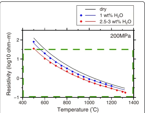
The C-2 conductor is distributed beneath Mt. Kuri-koma, which has displayed Quaternary volcanic activity (Fujinawa et al. 2001). Okada et al. (2010) indicated a low-velocity (Vs) anomaly in this area that was inter-preted as partial melting. They inferred that the melt originated from upwelling flow in the mantle wedge (e.g., Hasegawa et al. 2005). Thus, C-2 can be interpreted as high-temperature or partial melt zones related to vol-canic activities. Assuming that C-2 consists of a silicic

composition and contains 2.5 to 3.0 wt% or 0 wt% H2O,

the temperature of C-2 (<30Ω m) would be 500°C or

600°C, respectively, based on Gaillard (2004) (Figure 6). Similarly, the temperature of C-3a (<30Ωm), which is

−1 0 1 2

Resistivity (log10 ohm−m)

400 600 800 1000 1200 1400

Temperature (O

C)

dry

2.5-3 wt% H2O

1 wt% H2O

200MPa

Figure 6Resistivity of obsidians based on Figure seven in

Gaillard (2004).Diamonds denote laboratory measurements of

distributed beneath the Onikobe Caldera, should be more than 500°C. In contrast, the temperature in the non-volcanic area of the non-volcanic front area at a depth of 8 km

should be 210°C, assuming a heat flow of 80 mW/m2

(based on Tanaka and Ishikawa (2002) and Tanaka et al. (2004)). Therefore, the temperature in the areas of the C-2 and C-3a conductors should be 200°C higher than that of the surrounding area, assuming that high temperature causes the conductive anomalies. The actual temperature in the areas of the C-2 and C-3a conductors, however, should be higher than these estimates for the following reasons: (1) andesite, which requires a higher temperature to explain the same resistivity, as compared to silicic material (e.g., Gaillard and Marziano 2005), is distributed in the Kurikoma volcano (Fujinawa et al. 2001) and (2) the actual resistivity in the conductive areas should, in part, be

lower than 30Ω m because the inverted model shows a

value of 1Ωm in the centers of the C-2 and C-3a conduc-tors and the inversion adopted a smoothness constraint. Partial melt or a large amount of aqueous fluid may be re-quired to explain such a low resistivity. For better con-straint, additional surveys are required, especially for the C-3a conductor, which does not include an MT station.

The C-4 conductor is possibly required to explain out-of-quadrant phases in the YX component at sites Y200, Y210, and Y220 because the anomalous large phases are not explained when the C-4 conductor is filled with 300 Ωm (Figure 3). Similarly, out-of-quadrant phases observed at site I823 are not explained when C-5 is filled with 300

Ωm (Figure 3). On the other hand, strong channeling of

telluric current due to the shallow conductor beneath the Kitakami Lowland (C-1) is also a candidate for the anomal-ous large phases because a shallow conductor complex sometimes induces out-of-quadrant phases (e.g., Ichihara and Mogi 2009; Ichihara et al. 2013). Indeed, the above hy-pothesis model that the conductor is inserted in the blank areas of the MT sites (Figure 4) increases YX phase in the anomalous phase areas (Figure 3). However, the true resist-ivity distribution around the Kitakami Lowland is difficult to obtain based on the present data because the shallow re-sistivity distribution is not constrained in the blank area of MT stations, as we discussed previously.

The aftershocks are dominantly distributed in the resistive zone but are slightly within the C-1 and C-2 conductors. Because these are interpreted as granitic and Tertiary sedimentary rocks and high-temperature areas, respectively, the aftershocks occurred in brittle areas but rarely in ductile areas. This indicates that the seismicity depended highly on three-dimensional elastic

heterogeneity. As mentioned in the ‘Introduction,’ the

magnitude and rupture area of the 2008 Iwate-Miyagi Nairiku earthquake (M 7.2) are anomalously large for an earthquake occurring in a volcanic area where ductile zones are generally distributed. However, this study has

indicated that the ductile zones related to volcanic activ-ities are patchily distributed and that the size of the brittle area is large enough for M 7-class earthquakes to occur. These elastic heterogeneities may also have been respon-sible for the earthquake occurrence in a different way be-cause elastic heterogeneities may result in local stress concentration zones and can cause faulting (e.g., Ichihara et al. 2008, 2013; Iio et al. 2002). These interpretations imply that the MT method can detect elastic heterogene-ities that may control the occurrence and magnitude of the large inland earthquakes. Therefore, three-dimensional re-sistivity modeling based on MT surveying is important for understanding earthquake occurrences.

Conclusion

We conducted magnetotelluric surveys at 14 stations around the focal area of the 2008 Iwate-Miyagi Nairiku earthquake (M 7.2). Based on the MT impedances along four profiles by the present and previous studies, a prelim-inary 3-D resistivity model was obtained using WSINV3D code. The resistivity model showed a shallow conductive zone (C-1) and a few distinct conductive areas around the focal area (C-2, C-3a, C-4, and C-5). C-1 was interpreted as Tertiary sediment based on its geological distribution. C-2 and C-3a possibly indicate high-temperature zones re-lated to volcanic activities beneath Mt. Kurikoma and Oni-kobe Caldera. Aftershocks were distributed mainly in the resistive zone and not in the aforementioned conductive zones, which implies that elastic heterogeneity due to vol-canic activity and geology may control the magnitude and occurrence frequency of such earthquakes. However, this study could not constrain the precise resistivity distribu-tion in the blank areas of MT stadistribu-tions. Thus, dense surveys between the existing profiles of MT stations are required for more detailed interpretations.

Competing interests

The authors declare that they have no competing interests.

Authors’contributions

HI (corresponding author) participated in the acquisition, analysis, and interpretation of data, and drafted the manuscript. SS, MM, MU, TN, YO, YY, and TM (Toru Mogi) participated in the acquisition and interpretation of data. KA and TM (Takuya Miura) participated in the acquisition of data. All authors read and approved the final manuscript.

Acknowledgements

Author details 1

Research and Development Center for Earthquake and Tsunami, Japan Agency for Marine-Earth Science and Technology, Yokosuka 237-0061, Japan. 2

Earthquake Research Institute, The University of Tokyo, Tokyo 113-0032, Japan.3_{Faculty of International Resource Sciences, Akita University, Akita} 010-8502, Japan.4Research Center for Prediction of Earthquakes and Volcanic Eruptions, Graduate School of Science, Tohoku University, Sendai 980-8578, Japan.5Volcanic Fluid Research Center, Tokyo Institute of Technology, Tokyo 152-8551, Japan.6_{Institute of Geology and Geoinformation, National Institute} of Advanced Industrial Science and Technology (AIST), Tsukuba 305-8567, Japan.7_{Institute of Seismology and Volcanology, Graduate School of Science,} Hokkaido University, Sapporo 060-0810, Japan.8Current address: JGI, Inc., Tokyo 112-0012, Japan.

Received: 11 December 2013 Accepted: 26 May 2014 Published: 10 June 2014

References

Caldwell TG, Bibby HM, Brown C (2004) The magnetotelluric phase tensor. Geophys J Int 158(2):457_–469

Fujinawa A, Fujita K, Takahashi M, Umeda K, Hayashi S (2001) Development history of Kurikoma Volcano, Northeast Japan. Bull Volcanological Soc Japan 46:269_–284

Gaillard F (2004) Laboratory measurements of electrical conductivity of hydrous and dry silicic melts under pressure. Earth Planet Sci Lett 218(1–2):215–228, doi:10.1016/S0012-821x(03)00639-3

Gaillard F, Marziano GI (2005) Electrical conductivity of magma in the course of crystallization controlled by their residual liquid composition. J Geophys Res 110(B6), B06204, doi:10.1029/2004jb003282

Gamble TD, Clarke J, Goubau WM (1979) Magnetotellurics with a remote magnetic reference. Geophysics 44(1):53_–68

Hasegawa A, Nakajima J, Umino N, Miura S (2005) Deep structure of the northeastern Japan arc and its implications for crustal deformation and shallow seismic activity. Tectonophysics 403(1_–4):59_–75

Ichihara H, Mogi T (2009) A realistic 3-D resistivity model explaining anomalous large magnetotelluric phases: the L-shaped conductor model. Geophys J Int 179(1):14–17, doi:10.1111/J.1365-246x.2009.04310.X

Ichihara H, Honda R, Mogi T, Hase H, Kamiyama H, Yamaya Y, Ogawa Y (2008) Resistivity structure around the focal area of the 2004 Rumoi-Nanbu earthquake (M 6.1), northern Hokkaido, Japan. Earth Planets Space 60(8):883–888 Ichihara H, Mogi T, Hase H, Watanabe T, Yamaya Y (2009) Resistivity and density

modelling in the 1938 Kutcharo earthquake source area along a large caldera boundary. Earth Planets Space 61(3):345–356, doi:10.1016/J. Tecto.2013.05.020

Ichihara H, Uyeshima M, Sakanaka S, Ogawa T, Mishina M, Ogawa Y, Nishitani T, Yamaya Y, Watanabe A, Morita Y, Yoshimura R, Usui Y (2011) A fault-zone conductor beneath a compressional inversion zone, northeastern Honshu, Japan. Geophys Res Lett 38, L09301, doi:10.1029/2011gl047382

Ichihara H, Mogi T, Yamaya Y (2013) Three-dimensional resistivity modelling of a seismogenic area in an oblique subduction zone in the western Kurile arc: constraints from anomalous magnetotelluric phases. Tectonophysics 603:114–122, doi:10.1016/J.Tecto.2013.05.020

Iio Y, Sagiya T, Kobayashi Y, Shiozaki I (2002) Water-weakened lower crust and its role in the concentrated deformation in the Japanese Islands. Earth Planet Sci Lett 203(1):245–253

Kato N, Sato H, Umino N (2006) Fault reactivation and active tectonics on the fore-arc side of the back-arc rift system, NE Japan. J Struct Geol 28(11):2011–2022, doi:10.1016/J.Jsg.2006.08.004

Mishina M (2009) Distribution of crustal fluids in Northeast Japan as inferred from resistivity surveys. Gondwana Res 16(3–4):563–571, doi:10.1016/J.Gr.2009.02.005 Mitsuhata Y, Ogawa Y, Mishina M, Kono T, Yokokura T, Uchida T (2001)

Electromagnetic heterogeneity of the seismogenic region of 1962 M6.5 northern Miyagi earthquake, northeastern Japan. Geophys Res Lett 28(23):4371_–4374

Miura S, Sato T, Tachibana K, Satake Y, Hasegawa A (2002) Strain accumulation in and around Ou Backbone Range, northeastern Japan as observed by a dense GPS network. Earth Planets Space 54(11):1071_–1076

Miura S, Sato T, Hasegawa A, Suwa Y, Tachibana K, Yui S (2004) Strain concentration zone along the volcanic front derived by GPS observations in NE Japan arc. Earth Planets Space 56(12):1347–1355

Ogawa Y, Mishina M, Goto T, Satoh H, Oshiman N, Kasaya T, Takahashi Y, Nishitani T, Sakanaka S, Uyeshima M, Takahashi Y, Honkura Y, Matsushima M (2001) Magnetotelluric imaging of fluids in intraplate earthquake zones, NE Japan back arc. Geophys Res Lett 28(19):3741–3744

Okada T, Umino N, Hasegawa A (2010) Deep structure of the Ou mountain range strain concentration zone and the focal area of the 2008 Iwate-Miyagi Nairiku earthquake, NE Japan—seismogenesis related with magma and crustal fluid. Earth Planets Space 62(3):347–352, doi:10.5047/Eps.2009.11.005

Okada T, Umino N, Hasegawa A, Group for the aftershock observations of the Iwate-Miyagi Nairiku Earthquake in 2008 (2012) Hypocenter distribution and heterogeneous seismic velocity structure in and around the focal area of the 2008 Iwate-Miyagi Nairiku Earthquake, NE Japan—possible seismological evidence for a fluid driven compressional inversion earthquake. Earth Planets Space 64(9):717–728, doi:10.5047/Eps.2012.03.005

Parkinson WD (1962) The influence of continents and oceans on geomagnetic variations. Geophys J Roy Astr S 6(4):441–449

Sarma SVS, Prasanta B, Patro K, Harinarayana T, Veeraswamy K, Sastry RS, Sarma MVC (2004) A magnetotelluric (MT) study across the Koyna seismic zone, western India: evidence for block structure. Phys Earth Planet Inter 142(1–2):23–36, doi:10.1016/J.Pepi.2003.12.005

Sato H (1994) The relationship between Late Cenozoic tectonic events and stress-field and basin development in northeast Japan. J Geophys Res 99(B11):22261–22274

Siripunvaraporn W, Egbert G, Lenbury Y, Uyeshima M (2005a) Three-dimensional magnetotelluric inversion: data-space method. Phys Earth Planet Inter 150(1–3):3–14

Siripunvaraporn W, Egbert G, Uyeshima M (2005b) Interpretation of two-dimensional magnetotelluric profile data with three-dimensional inversion: synthetic examples. Geophys J Int 160(3):804–814

Takakura S (1995) Resistivity of Neogene rocks on the Niigata and the Akita oil fields, Japan. Butsuri-Tansa 48:161–175 (in Japanese with English abstract) Tanaka A, Ishikawa Y (2002) Temperature distribution and focal depth in the crust

of the northeastern Japan. Earth Planets Space 54(11):1109–1113 Tanaka A, Yamano M, Yano Y, Sawada M (2004) Digital Geoscience Map P-5:

geothermal gradient and heat flow data in and around Japan. Chishitsu News 603:42–45

Toh H, Baba K, Ichiki M, Motobayashi T, Ogawa Y, Mishina M, Takahashi I (2006) Two-dimensional electrical section beneath the eastern margin of Japan Sea. Geophys Res Lett 33(22), L22309, doi:10.1029/2006GL027435

Unsworth M, Bedrosian PA (2004) Electrical resistivity structure at the SAFOD site from magnetotelluric exploration. Geophys Res Lett 31:L12S05, doi:10.1029/2003GL019405

Wannamaker PE, Caldwell TG, Jiracek GR, Maris V, Hill GJ, Ogawa Y, Bibby HM, Bennie SL, Heise W (2009) Fluid and deformation regime of an advancing subduction system at Marlborough, New Zealand. Nature 460(7256):733–U790, doi:10.1038/Nature08204

Wessel P, Smith WHF (1998) New, improved version of the Generic Mapping Tools released. EOS Trans AGU 79:579

Yoshimura R, Oshiman N, Uyeshima M, Toh H, Uto T, Kanezaki H, Mochido Y, Aizawa K, Ogawa Y, Nishitani T, Sakanaka S, Mishina M, Satoh H, Goto T, Kasaya T, Yamaguchi S, Murakami H, Mogi T, Yamaya Y, Harada M, Shiozaki I, Honkura Y, Koyama S, Nakao S, Wada Y, Fujita Y (2009) Magnetotelluric transect across the Niigata-Kobe Tectonic Zone, central Japan: a clear correlation between strain accumulation and resistivity structure. Geophys Res Lett 36, L20311, doi:10.1029/2009gl040016

doi:10.1186/1880-5981-66-50