Range free localization using expected hop progress in anisotropic wireless sensor networks

R E S E A R C H

Open Access

Range-free localization using expected hop

progress in anisotropic wireless sensor

networks

Wu Wen

, Xianbin Wen

, Liming Yuan

and Haixia Xu

Abstract

Accurate localization of nodes is one of the key issues of wireless sensor network (WSN). A localization algorithm using expected hop progress (LAEP) has been successfully applied in isotropic wireless sensor networks. However, range-free LAEP cannot be directly used for anisotropic WSNs because anisotropic problems limit the applicability of multi-hop localization. In order to solve the problem, an improved localization algorithm is proposed to reduce the localization error. In this paper, we adapt the expected hop progress to anisotropic WSNs by considering both hop count computation and anchor selection. Then, particle swarm optimization algorithm is introduced to improve the positioning accuracy. The experimental results demonstrate that our algorithm has better higher precision than do state-of-the-art algorithms. Even for isotropic WSNs, our algorithm always outperforms its counterparts.

Keywords:Anisotropic wireless sensor networks, Range-free, Multi-hop, Expected hop progress, Particle swarm optimization

1 Introduction

Wireless sensor networks (WSNs) are an emerging tech-nology that has potential applications in various fields, such as healthcare, surveillance, astronomy, military and agriculture [1–4]. Most of these applications require knowledge of the exact locations of the sensor nodes used to sense the data. In the absence of such informa-tion, data may not be useful for users. Therefore, the precise localization of sensors is a critical requirement in WSNs [5].

The localization issue in WSNs can be resolved by using the global positioning system (GPS) with each sensor node, but this is not favourable due to energy, cost and size issues. An efficient and better alternative is required to localize the sensor nodes. Various non-GPS-based localization algorithms have been used, which are catego-rized into range-based [6, 7] and range-free [8, 9] algo-rithms. Although the range-based algorithms are more accurate than the range-free localization algorithms, they

require a very high cost. Unlike range-based algorithms, range-free algorithms, which rely on the network connect-ivity to estimate the positions of regular nodes without any extra hardware supporting, are more power-efficient and do not require additional hardware. At present, most researchers focus on isotropic WSNs. Wireless sensor net-works are mostly applied to complex environments where there are obstacles and holes, in which case they are called anisotropic wireless sensor networks (AWSNs). In this case, when the line connecting two nodes passes these ob-stacles, the shortest paths between anchor nodes and regular nodes are likely to be curved and its length may be estimated much larger than corresponding Euclidean dis-tance. Therefore, position estimation is inaccurate.

DV-Hop [10], Amorphous [11], MDS-MAP [12] and APIT [13] are examples of early range-free localization schemes that are well suited for isotropic wireless net-works (i.e. where obstacles do not exist). However, the distance estimation accuracy of these methods is se-verely degraded in anisotropic networks, resulting in un-acceptable overall localization errors. To solve this problem, a few new range-free algorithms are proposed for tolerating erroneous distance estimates in AWSNs. * Correspondence:[email protected];[email protected]

1_{Key Laboratory of Computer Vision and System, Ministry of Education,}

Tianjin University of Technology, Tianjin 300384, China Full list of author information is available at the end of the article

The proximity distance mapping (PDM) [14] algorithm

replaces the average hop distance with a

proximity-distance mapping matrix in estimating the distances between nodes and anchors. Substantial topo-logical information can be preserved by the mapping matrix. The pattern-driven scheme (PDS) [15] algorithm applies various distance estimation algorithms for chors based on their exhibited patterns. Next, the an-chor supervised [16] algorithm is presented. In this approach, every anchor selects a set of reliable anchors for which distance estimates can be accurately obtained. Later, a location algorithm that uses the expected hop progress (EHP) was proposed in [17, 18]. A modified EHP approach is obtained by redefining a new cumula-tive distribution function (CDF) and achieves satisfactory localization results [19]. The algorithm depends not only on the communication radius of the anchors, but also on the communication radius of the inter-nodes, which is closer to the real Euclidean distance between any two nodes. Recently, Farrukh Shahzad proposed a scheme, called DV-maxHop [20], that can achieve similar or bet-ter performance by just introducing a control paramebet-ter

MaxHop in the first phase of the DV-Hop algorithm. However, most of these methods do not achieve better positioning accuracy or achieve better accuracy at the expense of high computational or communication over-heads. Therefore, a low-cost and high-precision algo-rithm for anisotropic WSNs is necessary.

In this paper, we propose a novel range-free

localization algorithm based on the modified EHP and a particle swarm optimization algorithm (PSO) [21] that is tailored for anisotropic WSNs. First, we assume that the degree of irregularity (DOI) of the communication ra-dius is equal to zero. Then, the distance from regular nodes to reliable anchors can be estimated precisely by introducing a control parameter, MaxHop. The reliable anchors are properly chosen following a new reliable an-chor selection strategy. Next, we use the mathematical expectation of CDF to estimate the distances between the regular nodes and the reliable anchors. Finally, the PSO algorithm is used for localization optimization.

The organization of this paper is as follows. Section2 presents the localization model of multi-hop AWSN. Then, the proposed range-free localization algorithm and PSO algorithm are proposed in this section. The simula-tion results and performance evaluasimula-tions are analysed in Section3. Finally, Section4concludes the paper.

2 Methodology

2.1 Network model and overview

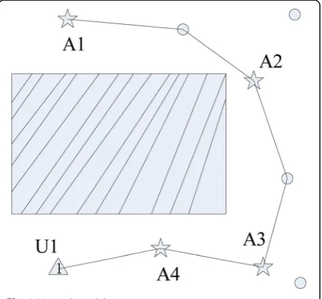
For our study, wireless nodes are deployed in a two-dimensional (2-D) square area. In the anisotropic net-work case, there are one or two rectangular structures or holes where nodes cannot be deployed. As shown in Fig.1,

under such anisotropic terrain conditions,Nsensor nodes are uniformly deployed in a square areaSthat contains a rectangular obstacle, which form a C-shaped network top-ology. The signal does not pass through these obstacles. All nodes are assumed to have the same transmission capability, except when we consider the effect of DOI during simulation. Each node can directly communi-cate with any other node in the disc, with that node as the centre and radius. Each anchor node is equipped with a GPS receiver, and they are aware of their positions. The other nodes, called regular nodes, do not know their own positions [22, 23].

The major symbols used in this paper are listed as follows:

N= the total number of all nodes;

Na= the number of anchor nodes (ANs);

Nu= the number of unknown nodes (UNs);

R= the communication range or radius of each node (m);

λ= the node density in the monitoring area;

area(k,R) = thek-th node’s coverage area with thek-th sensor as the centre and radiusR.

In multi-hop AWSN localization, the goal is to esti-mate the locations of all UNs by using ANs and partial information of the distances between various pairs of ANs and UNs. We suppose that the i-th anchor node broadcasts data packet containing its position and the

j-th regular node receives the data packet through multi-hop communication. Then, we employ the short-est path method to obtain a possible path between a source sensor and a destination sensor with the

minimum number of hops. Let nij be the number of hops between the i-th anchor and thej-th regular node. The distance d^i−j from the j-th regular node to the i-th anchor is estimated as follows [24]:

^

di−j¼nijhs ð1Þ

wherehsis a predefined average hop distance. To a large

extent, this distance estimation approach relies on the high density of WSNs.

Although heuristic and analytical algorithms are proven to be sufficiently accurate in isotropic WSNs, their accuracies are not optimal in anisotropic WSNs. It is very likely that the shortest path between an anchor node and a regular node is curved in an AWSN, thereby resulting in an overestimation of the hop count between these two nodes. According to Fig. 1, the hop size be-tween nodesA1andU1is six hops; however, the number of hops between them is far smaller due to obstacles. The larger the hop size estimation errors are, the greater the distance estimation errors are, and consequently, the less accurate the localization is. To solve this problem, we propose a novel localization algorithm that is based on new reliable anchor selection strategy. We introduce a parameterMaxHopin the first phase of our algorithm. The algorithm ignores the information if the hop count is greater than MaxHop. In the anisotropic network, when two nodes locate at two ends of an obstacle group, we ignore the farther anchor which will cause a detoured path, and consequently, the shortest path between two nodes will not be curved. Then, the EHP method is adopted to calculate the average hop distance. In Fig.1, regular node U1 will select A4 and A3 as reliable an-chors. We can use the average hop distance to make the distance calculation among regular nodeU1and reliable anchors more precise in AWSNs. In the next section, we derive the expression for hsthat is exploited later in our algorithm.

2.2 The proposed algorithm and its analysis

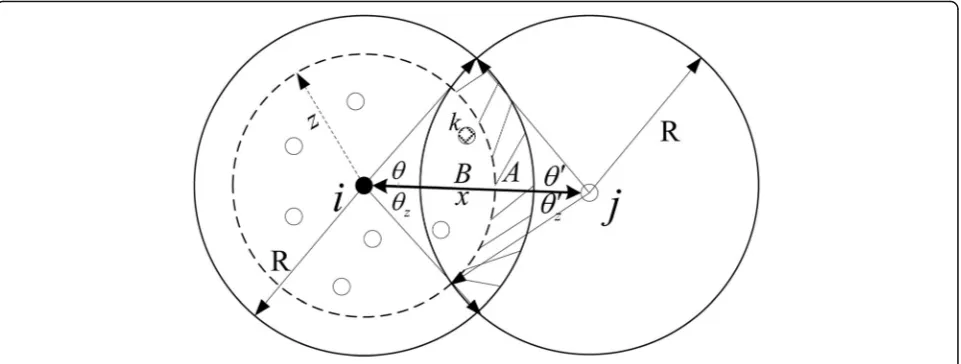
2.2.1 Hop distance derivation using the EHP approach The EHP algorithm is based on an accurate analysis of hop progress in WSNs. We can derive the distance be-tween any two nodes through expected hop progress. In the network model with uniform sensor transmission range and arbitrary node density, the expected hop pro-gress of each hop in this network is the same. Therefore, the expected hop progress can be used to replace the average hop distance. In this section, for the sake of clar-ity, we discuss only two-hop communication in which the i-th node communicates with thej-th node through an intermediate node k. For clarity, let the random vari-ables X and Z represent the distances di-j and di-k,

respectively. Then, we use the expectation of Z to represent the average hop distance, as shown in for-mula (2) [25].

hs¼E Zf g ð2Þ

To obtain a more accurate value for hs, we use the conditional cumulative distribution function (CDF) FZ∣

X(z) =P(Z≤z|x) of Z to represent the average hop dis-tance. In Fig. 2, ifZ≤z is guaranteed, then there are no nodes in the dashed area A. We define the conditional CDF in formula (3).

FZjXð Þ ¼z P Zð ≤zjxÞ ¼P Að 0jQ1Þ ð3Þ

whereQ1is the potential forwarding area wherein thek

-th node communicates directly wi-th -the j-th and i-th nodes andP(A0|Q1) is the probability that event A0

oc-curs given eventQ1.A0indicates that there are no nodes

in the dashed area A, and Q1 indicates that there is at

least one node in the potential forwarding areaQ, which depends on communication radius R. The potential for-warding areaQis given by formula (4).

Q¼areaði;RÞ∩areaðj;RÞ ¼A∪B ð4Þ

The probability of there being Knodes in area A fol-lows the binomial distribution X~B(N, p), where p = A/ S. For relatively largeN and smallp,B(N,p) can be ac-curately approximated by a Poisson distribution, as shown in formula (5).

FZjXð Þ ¼Z e−λA ð5Þ

where λ= N/S is the average node density of the net-work. We can easily calculate the area of A using geo-metrical properties and trigonometric transformations. It is straightforward to show that:

A¼R2 θþθ0þθ0z−

per-hop distance increases if the number of nodes lo-cated inside Q increases. According to formula (8), hs can be derived if the node density and the transmission range are given. In this way, a more accurate average hop distance can be easily obtained in AWSNs through finite integrals.

When hs is determined, each unknown node collects the gradients of all its neighbouring nodes relative to an anchor node and uses the local mean to replace the hop counts. As shown in formula (9), the Amorphous method is adopted to calculate the minimum hops from nodejto anchor nodes and the minimum hops is reduced by 0.5 through previous experimental statistics [7].

Sj¼

where hjand hj' are the smallest hop counts of the

un-known node jand the neighbouring node of node j, re-spectively, to the anchor node;neighbours(j) is the set of all neighbouring nodes of nodej.

2.2.2 Anchor selection strategy

In general, the greater the hop count between two nodes, the higher the distance estimation error in the AWSN. To solve this problem, we propose a new reli-able anchor selection strategy in which a hop size threshold is set; we call this parameter MaxHop [20]. When a node receives the position of any anchor with its hop count, the algorithm ignores the information if the hop count is greater than MaxHop; consequently, the information is not propagated further. This algo-rithm reduces the superposition of this cumulative error, improves the positioning accuracy, and reduces the net-work traffic. To obtain better positioning accuracy and low overheads, the threshold MaxHop should be set as close as possible to the smallest integer value on the basis of the successful positioning of all nodes.

The size of the hop threshold MaxHop is mainly

determined by the connectivity and anchor node density of the network. Its expression can be derived as follows [27]:

an experiment to further explore the appropriate value of the threshold MaxHop. Then, we use the corrected hop counts and formula (1) to estimate the distances between the unknown nodes and the anchor nodes.

2.2.3 Particle swarm optimization

PSO is an optimization algorithm that was proposed by American researchers in 1995 for mimicking the collective behavior of intelligent animals. The PSO searches the space of a fitness function by adjusting the trajectory of individual particles. In other words, the purpose of this algorithm is to find the global optimum until the fitness function no longer im-proves. We use the position of the best particle after a fixed number of iterations as the estimated location of the target. The advantages of this algorithm are as follows: provides fast convergence and high accuracy, is easy to implement and requires few parameters [28, 29]. In most applications, PSO is used as an evolu-tionary computation technology. The main steps of the PSO algorithm are as follows:

1. InitializeMparticles. The particle iteration number is expressed ast. In the search space, the position and velocity are expressed as formula (11).

Xt_a¼xt_a1;xt_a2

Vt_a¼vt_a1;vt_a2 ; a¼1;2;…;M ð11Þ

whereXt_a is the current position of particle (a),Vt_a is the velocity vector of particle a, and M is the total number of particles.

2. Select a suitable fitness function. It is used to judge the individuals in the population.

3. Update the velocity and position of the particle. At each iteration number (t+ 1), the velocity and position of particle (a) are updated according to the following two equations:

where pbest is the individual extremum, gbest is the glo-bal extremum, and c1and c2are cognition coefficients, which are random values in the range (0, 2).

4. Judge whether the termination conditions are satisfied. If the conditions are satisfied, the cycle is

terminated; otherwise, step 2 and step 3 are repeated.

5. Select the global extremum. When the maximum number of iterations is reached, the value of gbest that is selected by the fitness function is used as the estimated coordinates of the unknown nodes.

PSO is widely used in various fields, but less research has been conducted on the particle swarm optimization algorithm in AWSNs. The localization problem can be regarded as an optimization problem, and we can use PSO to correct the estimated positions. Therefore, we mainly study the optimization effect of PSO on the posi-tioning accuracy under the AWSN environment. In this process, it is very important to determine the fitness function. PSO begins with a group of random particles and finds the optimal solution through an iterative process. In the iterative process, the particle updates it-self by tracking “two optimal solutions”: one is the opti-mal solution obtained by the particle, namely, the local best position, and the other is the optimal solution ob-tained by the entire particle group, namely, the global best position. The position of the optimal particle is the coordinate position of the unknown node. Thus, the se-lection of the fitness function will directly affect the po-sitioning accuracy. The distance error between the anchor nodes is usually used as a fitness function, as shown by formula (13).

wherex andy are the coordinates of the particle,xiand yi are the coordinates of node i, fi is the absolute value of the distance error between beacon nodeito particlea and unknown nodej,η= 1/hopirepresents weight values for each anchor node, and fitness (x,y) is the particle fit-ness function. The detailed pseudo-code of the proposed algorithm, which is based on EHP and PSO, is described in Table1.

3 Experimental results and discussions

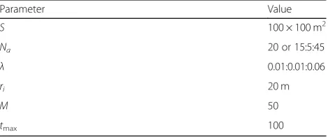
topology that is commonly used in the context of WSNs, namely, the C-shaped topology, as shown in Fig. 1. In addition, we examine the performance of the algorithm in the isotropic network. We always assume that the number of anchors Na is set to 20 and that the total number of nodes N is set to 100, 200, ..., 500, and 600. The transmission capability of R= 20 m is the same across the network. All simulation parameters are sum-marized in Table 2, and the simulation results are ob-tained by averaging over 100 trials.

To evaluate the performance of the proposed algo-rithm, three metrics are utilized, which are defined as follows:

Localization error

The localization error is the sum of the distances be-tween the nodes’ actual positions (xj,yj) and estimated positions ð^xj;^yjÞ, divided by the product of the number of location nodesNand the communication radiusR. It represents the position estimation deviation with respect to the transmission range, and we use the normalized root-mean-square error (NRMSE), which is defined as follows:

NRMSE¼

XN

j¼1

ffiffiffiffiffiffiffiffiffiffiffiffiffiffiffiffiffiffiffiffiffiffiffiffiffiffiffiffiffiffiffiffiffiffiffiffiffiffiffiffiffi

xj−^xj

2_þ

y_j−^y_j

2

r

NR ð14Þ

Distance error

Table 1Pseudo code of localization algorithm

Table 2Simulation parameters

Parameter Value

S 100 × 100 m2

Na 20 or 15:5:45

λ 0.01:0.01:0.06

ri 20 m

M 50

The size of the distance error directly affects the localization error. The distance error is the difference between the actual distance and the estimated distance between the two nodes, which can be represented by the mean distance error (MDE) and the distance estimation error (DER), as defined in formula (15) and formula (16), respectively.

MDE¼

XNa

i¼1 XNL

j¼1

di−j−^di−j

NaNL

ð15Þ

DER¼

di−j−^di−j

di−j

ð16Þ

whereNais the total number of anchor nodes; ^di−j and

di−j are the estimated distance and actual distance, re-spectively, between anchor nodei and unknown node j. MDE refers to the average distance error from nodeito j, and DER indicates the relative error between the esti-mated distance and the true distance.

Localization percentage

Due to the hop threshold limit, the percentage of unknown nodes for successful positioning cannot be 100% because this would result in the absence of anchor nodes. However, the percentage of positioning nodes is an important index for evaluating the

localization algorithm. The localization percentage can be expressed as follows:

localizable percentage¼NL Nu

100% ð17Þ

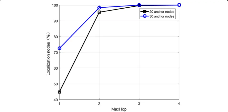
3.1 Select the appropriate value ofMaxHop

For the successful positioning of all nodes, the thresh-old MaxHop should be as close as possible to the smallest integer value. This will not only improve the positioning accuracy but also reduce the computa-tional and communication overheads. However, ac-cording to formula (10), the calculated values of

MaxHop are often too small. Figure 3 illustrates that the localization nodes’ percentage increases with an

increasing hop threshold MaxHop. This is because

the larger the hop threshold MaxHop is, the more re-liable the selected anchor nodes are. When enough anchor nodes are used to locate an unknown node, the probability of the unknown node being success-fully positioned increases. According to this figure, when MaxHop is equal to 3, the localization node percentage is close to 100%, regardless of whether the number of anchor nodes in the network is set to 20 or 30. Therefore, we should appropriately increase

MaxHop to meet the positioning requirements. In our

experiments, we always choose the value of MaxHop

to be 3.

3.2 Comparison of MDE and NRMSE with various node densities

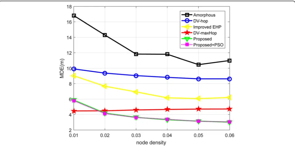
Figure 4 shows the localization MDEs achieved by

Amorphous, DV-Hop, improved EHP, DV-maxHop, pro-posed and propro-posed-PSO for various node densities. The MDE decreases as the node connectivity increases. According to this figure, the results demonstrate that the MDE of the proposed algorithm is less than those of its counterparts under the same network settings. How-ever, when the node density is low, the DV-maxHop al-gorithm outperforms our alal-gorithm. The MDE of the proposed and proposed-PSO algorithms are approxi-mately the same because the two algorithms use the same method to calculate the distance between nodes. In determining the location of a node, the proposed al-gorithm uses maximum likelihood estimation, and the proposed-PSO algorithm uses the PSO algorithm.

Next, we discuss the localization errors of the pro-posed algorithm and other algorithms under different node densities. According to Fig. 5, the proposed algo-rithm, with or without the PSO algoalgo-rithm, always out-performs its counterparts. Our proposed algorithm is approximately two, four, and five times more accurate

than DV-maxHop, improved EHP, DV-Hop, and

Amorphous, respectively. Furthermore, from this fig-ure, the NRMSE that is achieved by the proposed al-gorithm slightly decreases and then quickly saturates when the node density λ increases compared to other algorithms. This is expected since the approximation in formula (1) is more realistic when λ is large.

Hence, more accurate localization is achieved. At smaller node densities, the algorithm can also obtain satisfactory results. This indicates that this algorithm can achieve accurate positioning at smaller anchor node density, thereby reducing the localization cost of wireless sensor nodes. This further demonstrates the efficiency and suitability of the proposed localization algorithm in AWSNs.

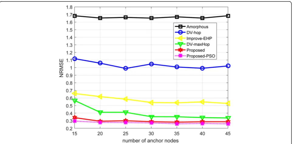
3.3 Influence of the number of anchor nodes and iteration times

In anisotropic networks, the node density is set to 0.06, and the communication radius is set to 20. Figure 6 shows the NRMSE achieved by Amorphous, DV-Hop, improved EHP, DV-maxHop, proposed and proposed-PSO when the number of anchor nodes is varied from 15 to 45. When the number of anchor nodes is less than 15 (the density of the anchors is less than 0.0015), the percentage of regular nodes for successful positioning cannot be 100% due to the absence of anchor nodes. The NRMSE achieved by the proposed algorithms sig-nificantly decreases initially and then decreases slightly when the number of anchor nodes increases. From the figure, the proposed-PSO algorithm outperforms the traditional algorithms in terms of accuracy.

Figure 7 illustrates the energy consumption and

localization NRMSE with different iteration numbers. We can see that with iterations increasing, the PSO al-gorithm can converge quickly to achieve higher accuracy in multi-hop AWSN localization. On the other hand, as

the number of iterations increases, so does the runtime, which means that the algorithm consumes more energy. Therefore, the faster convergence can enable us to save the searching overhead.

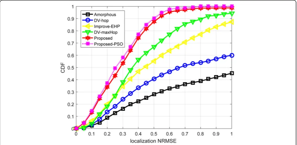
3.4 Comparison of localization NRMSE CDFs of various localization methods

In Fig.8, we first evaluated the localization results of the proposed algorithms by comparing them to those of

DV-maxHop, improved EHP, DV-Hop and Amorphous by utilizing cumulative distribution function plots. Using the proposed algorithm, 87% (90% with proposed-PSO) of the regular nodes could estimate their positions within almost a fifth of their transmission capabilities. In contrast, 67% of the nodes achieved the same accuracy as DV-maxHop, approximately 55% as improved EHP, approximately 40% as DV-Hop, and only 28% as Amorphous. This further demonstrates the efficiency of

Fig. 6NRMSE vs. number of anchor nodes in AWSN

the proposed localization algorithm and indicates that the proposed algorithm is more suitable for AWSNs.

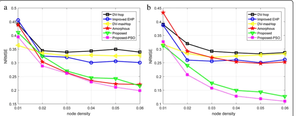
3.5 Precision analysis of the algorithms in an isotropic WSN

The algorithm we proposed above is also the most ac-curate in isotropic WSNs in which the nodes are uni-formly deployed in a 2-D square area S= 100 × 100 m2.

Under the same network settings but a different network topology, we have also carried out a series of experimen-tal studies. Figure 9 plots the localization NRMSEs achieved by Amorphous, DV-Hop, improved EHP, DV-maxHop and our proposed algorithms. According to this data, the localization error of the proposed-PSO algorithm is small in isotropic WSNs and the positioning accuracy is greatly increased in the middle square areaS Fig. 7The energy consumption and convergence analysis of PSO whenλ= 0.01

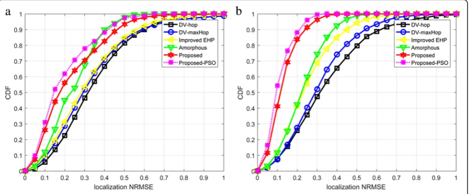
= 90 × 90 m2. This is because the approximation in for-mula (1) of the nodes in the middle of the region be-comes more realistic, which makes position estimation more accurate. In Fig.10, the NRMSEs of the two maps are 0.2013 and 0.1081. The localization accuracy in Fig.10b is higher than that in Fig.10a.

Figure11shows the localization NRMSE CDF under a node density of 0.06 for square area S= 100 × 100 m2 and square area S= 90 × 90 m2. According to this figure, the localization NRMSE CDF of Fig. 11b is far greater than that of Fig. 11a overall. Figure 11b shows that the NRMSE CDF of the proposed-PSO algorithm in the interval of length 0.3 is 99.49. This result indicates that the localization NRMSE of all nodes is less than 0.3.

This further demonstrates that our algorithm is the most accurate in isotropic WSNs, especially in the middle area

S= 90 × 90 m2.

4 Conclusion

In this paper, a novel range-free localization algorithm for multi-hop anisotropic wireless sensor networks is presented. The simulation result demonstrates that our modified algorithm has higher localization precision compared with state-of-the-art algorithms. In addition, our algorithm has achieved good results in isotropic WSNs, especially in the middle of the location area. In general, whether applied with or without the PSO algo-rithm, our proposed algorithm always outperforms the Fig. 9The influence of node density on NRMSE:aS= 100 × 100 m2;bS= 90 × 90 m2

most representative WSN localization algorithms. However, if the optimization algorithm is added, the en-ergy consumption will increase while increasing the localization accuracy. As a future work, we plan to study the heterogeneous wireless sensor networks where all nodes’ communication ranges are different and we are also planning to study the influence of the irregular communication range in AWSN.

Abbreviations

2-D:Two-dimensional; ANs: Anchor nodes; AWSN: Anisotropic wireless sensor network; CDF: Cumulative distribution function; DER: Distance estimation error; DOI: Degree of irregularity; EHP: Expected hop progress; GPS: Global positioning system; LAEP: Localization algorithm using expected hop progress; MDE: Mean distance error; NRMSE: Normalized root-mean-square error; PSO: Particle swarm optimization; UNs: Unknown nodes; WSN: Wireless sensor network

Acknowledgements

Not applicable.

Funding

This work is supported by National Natural Science Foundation of China (No. 61472278 and 61102125), Key project of Natural Science Foundation of Tianjin University (2017ZD13), the Research Project of Tianjin Municipal Education Commission (No. 2017KJ255).

Availability of data and materials

Not applicable.

Authors_’contributions

WW proposed the main idea and performed the simulation and manuscript writing. XW provided guidance for the algorithm design and helped revise the manuscript. All authors read and approved the final manuscript.

Authors’information

Wu Wen received his bachelor’s degree in communication engineering from Liaoning University of Technology in 2016. He is pursuing her master’s degree in communication and information engineering at Tianjin University of Technology, China. His research interests include anisotropic wireless sensor networks, wireless sensor networks localization and performance evaluation and optimization.

Xianbin Wen received his PhD from the Northwestern Polytechnical University, Xi’an, China, in 2005. He is currently a professor with the School of

Computer and Communication Engineering, Tianjin University of Technology, Tianjin, China. His research interests include image interpretation, machine learning, and information hiding.

Liming Yuan received the PhD degree in computer science and technology from Harbin Institute of Technology, China, in 2014. He is currently working as a lecturer in the School of Computer Science and Engineering at Tianjin University of Technology, China. His research interests are mainly in machine learning and image processing.

Haixia Xu received her MSc degree in applied mathematics from the Northwestern Polytechnical University, China, in 2006, and a PhD in computer science and technology from the same university in 2009. She is currently an associate professor at the School of Computer and

Communication Engineering, Tianjin University of Technology, China. Her main research interests include image analysis, signal processing, and pattern recognition.

Competing interests

The authors declare that they have no competing interests.

Publisher’s Note

Springer Nature remains neutral with regard to jurisdictional claims in published maps and institutional affiliations.

Author details

1_{Key Laboratory of Computer Vision and System, Ministry of Education,}

Tianjin University of Technology, Tianjin 300384, China.2_{Tianjin Key} Laboratory of Intelligence Computing and Novel Software Technology, Tianjin University of Technology, Tianjin 300384, China.

Received: 14 May 2018 Accepted: 11 December 2018

References

1. Y. Zhu, Y. Zhang, W. Xia, L. Shen, inA Software-Defined Network Based Node Selection Algorithm in WSN Localization. 83rd vehicular technology conference (Nanjing, 2016), pp. 1_–5

2. H. Zheng, W. Guo, N. Xiong, A kernel-based compressive sensing approach for mobile data gathering in wireless sensor network systems. IEEE Trans. Syst. Man Cybern. Syst.48(12), 1–13 (2017)

3. N. Xiong, X. Jia, L. Yang, A. Vasilakos, Y. Li, Y. Pan, A distributed efficient flow control scheme for multirate multicast networks. IEEE Trans. Parallel Distrib. Syst.21(9), 1254–1266 (2010)

4. B. Lin, W. Guo, N. Xiong, G. Chen, A. Vasilakos, H. Zhang, A pretreatment workflow scheduling approach for big data applications in multi-cloud environments. IEEE Trans. Netw. Serv. Manag.13(3), 581–594 (2016)

5. S. Tomic, M. Beko, R. Dinis, M. Tuba, N. Bacanin, inAn efficient WLS estimator for target localization in wireless sensor networks. 24th telecommunications forum (Belgrade, 2017), pp. 1–4

6. B. Xiao, L. Chen, Q. Xiao, Reliable anchor-based sensor localization in irregular areas. IEEE Trans. Mob. Comput.9(1), 60_–72 (2010)

7. L.Z. Zhao, X.B. Wen, D. LI, Amorphous localization algorithm based on BP artificial neural network. Int. J. Distrib. Sens. Netw (2015).https://doi.org/10.1155/2015/657241

8. T. Alhmiedat, A.A. Salem, A hybrid range-free localization algorithm for ZigBee wireless sensor networks. Int. Arab J. Inf. Technol14(4A), 647–653 (2017) 9. N.B.M. Ngabas, J.B. Abdullah, inComparison of energy consumption in

cooperative range-free localization for wireless sensor network. IEEE student conference on research and development (Putrajaya, 2013), pp. 459–464 10. Q.G. Gao, L. Lei,in 2nd International Conference on Advanced Computer

ControlAn improved node localization algorithm based on DV-HOP in WSN

(Shenyang, 2010), pp. 321–324

11. S. Shen, B. Yang, K. Qian, W. Wang, X. Jiang, Y. She, Y. Wang, inAn improved amorphous localization algorithm for wireless sensor networks. International conference on networking and network applications (Hakodate, 2016), pp. 69–72 12. X. Sun, T. Chen, W. Li, M. Zheng,in International Conference on Computer

Science and Electronics EngineeringPerfomance research of improved MDS-MAP algorithm in wireless sensor networks localization(Hangzhou, 2012), pp. 587–590 13. Y Zhou, X Ao, S Xia, in 7th World Congress on Intelligent Control and

Automation. An improved APIT node self-localization algorithm in WSN, (Chongqing, 2008), pp. 7582_–7586

14. H. Lim, J.C. Hou, inLocalization for anisotropic sensor networks. 24th annual joint conference of the IEEE computer and communications societies (Miami, 2005), pp. 138_–149

15. Q. Xiao, B. Xiao, J. Cao, J. Wang, Multihop range-free localization in anisotropic wireless sensor networks: a pattern-driven scheme. IEEE Trans. Mob. Comput.9(11), 1592_–1607 (2010)

16. X. Liu, S.G. Zhang, K. Bu, A locality-based range-free localization algorithm for anisotropic wireless sensor networks. Telecommun. Syst62(1), 3–13 (2016) 17. Y. Wang, X.D. Wang, D.M. Wang, D.P. Agrawal, Range-free localization using

expected hop progress in wireless sensor networks. IEEE Trans. Parallel Distrib. Syst20(10), 1540_–1552 (2009)

18. AE Assaf, S Zaidi, S Affes, N Kandil, in IEEE International Conference on Communications (ICC). Cost-effective and accurate nodes localization in heterogeneous wireless sensor networks. (London, 2015), pp. 6601_–6608 19. A.E. Assaf, S. Zaidi, S. Affes, N. Kandil, Low-cost localization for multihop heterogeneous

wireless sensor networks. IEEE Trans. Wirel. Commun.15(1), 472–484 (2016) 20. F. Shahzad, T. Shaltami, E. Shakshukhi, DV-maxHop: a fast and accurate

range-free localization algorithm for anisotropic wireless networks. IEEE Trans. Mob. Comput.16(9), 2494–2505 (2017)

21. F Zhou, S Chen, in Proceedings of the 2016 International Conference on Communications. DV-Hop Node Localization Algorithm Based on Improved Particle Swarm Optimization, (2016), pp. 541–550

22. W. WL, X.B. Wen, H.X. Xu, L.M. Yuan, Q.X. Meng, Efficient range-free localization using elliptical distance correction in heterogeneous wireless sensor networks. Int. J. Distrib. Sens. Netw. (2018).https://doi.org/10.1177/ 1550147718756274

23. W. WL, H.X.X. XB Wen, L.M. Yuan, Q.X. Meng, Accurate range-free localization based on quantum particle swarm optimization in heterogeneous wireless sensor networks. KSII Trans. Internet Inf. Syst.12(3), 1083–1097 (2018) 24. A.E. Assaf, S. Zaidi, S. Affes, N. Kandil, inAccurate Nodes Localization in

Anisotropic Wireless Sensor Networks. IEEE International Conference on Ubiquitous Wireless Broadband (ICUWB) (2015), pp. 1–5

25. A.E. Assaf, S. Zaidi, S. Affes, Robust ANNs-based WSN localization in the presence of anisotropic signal attenuation. IEEE Wirel. Commun. Lett5(5), 504_–507 (2016)

26. S Zaidi, AE Assaf, S Affes, N Kandil, in IEEE International Conference on Ubiquitous Wireless Broadband. Range-Free Nodes Localization in Mobile Wireless Sensor Networks, (2015), pp. 1_–6

27. Y. Yue, L. Ding, H. Zhao, H. Wang,in IEEE International Conference on Mechatronics and Automation (ICMAStudy on DV-HOP node location algorithm for Wireless Sensor Networks(Takamatsu, 2017), pp. 1709_–1713 28. R. Zhang, F. Yan, W. Xia, S. Xing, Y. Wu, L. Shen,An Optimal Roadside Unit

Placement Method for VANET Localization(Singapore, 2017), pp. 4–8.IEEE Global Communications Conference