Article
MHD Flow and Heat Transfer Analysis in Wire
Coating Process Using Elastic-Viscous Fluid
Zeeshan Khan 1,*, Rehan Ali Shah 2, Saeed Islam 3, Hamid Jan 1, Bilal Jan 1, Haroon-Ur Rasheed 1 and Aurangzeeb Khan 4
1 Sarhad university of Science and Information Technology, Peshawar 25000, KP, Pakistan;
[email protected] (H.J.); [email protected] (B.J.); [email protected] (H.R.)
2 Department of Mathematics, University of Engineering and Technology, Peshawar 25000, KP, Pakistan;
3 Department of Mathematics, Abdul Wali Khan University Mardan, Mardan 23200, KP, Pakistan;
4 Department of Physics, Abdul Wali Khan University Mardan, Mardan 23200, KP, Pakistan * Correspondence: [email protected]
Abstract: The most important plastic resins used for wire coating are Polyvinyl Chloride (PVC), Nylon, Polysulfone and Low-high density polyethylene (LDPE / HDPE). In this article,the coating process is performed using elastic-viscous fluid as a coating material for wire coating in a pressure type coating die. The elastic-viscous fluid is electrically conducted in the presence of an applied magnetic field. The governing non-linear equations are modeled and then solved analytically by utilizing an Adomian decomposition method (ADM). The convergence of the series solution is established. The results are also verified by Optimal Homotopy Asymptotic Method (OHAM). The effect of different emerging parameters such as non-Newtonian parameters α and β, magnetic parameter M and the Brinkman number Br on solutions (velocity and temperature profiles) are discussed through several graphs. Additionally, the current result also compares with the published work already available in the literature.
Keywords: wire coating; elastico-viscous fluid; MHD flow; heat transfer; ADM and OHAM
1. Introduction
Studying the boundary layer behavior of a viscoelastic fluid on a continuous stretching surface, it is important for the analysis of the extrusion of the polymer, stretching of plastic films, optical fibers and cables. The importance in industrial process applications has raised significant interest from researchers for the study of viscoelastic fluid flow and heat transfer in fiber or wire coating process. The metal coating is an industrial process for the supply of insulation, environmental safety, mechanical damage and protect against signal attenuation. The simple and appropriate process for wire coating is the coaxial extrusion process that operates at the maximum speed of pressure, temperature and wire drawing. This produces higher pressure in the particular region resulting into strong bond and rapid coating. Several studies like, Han and Rao [1], Nayal [2], Caswell [3] and Ticker [4] have focused on the co-extrusion process in which the fibers or wires are drawn inside the molten polymer filled in a die.
the oscillating boundary condition was investigated by Shah et al. [9, 10] for wire coating. The same author discussed the third grade fluid for wire coating.
Interest in heat transfer in Newtonian fluids have significantly increased the use of non-Newtonian fluids perpetuated through various industries, including processing of polymers and electronics packaging. The heat transfer analysis is significant for the technology and advancement of science and up to date instruments such as compact heat exchangers, laser coolant lines and micro-electro-mechanical systems (MEMS). A comprehensive survey of the literature is thus impractical.
However, some studies are listed here to provide a starting point for wider research literature. Shah et al. [12] studied wire-coating with a temperature varying linearly. Mitsoulis [13] has studied the flow of wire-coating with heat transfer. The heat transfer problem corresponding fully developed pipe and PTT fluid flow channels was also studied by Oliveira and Pinho [14].
The post-treatment of wire coating analysis also studied by many researchers [16]. Wagner et al. [17] investigated the wire coating with the effect of die design. Numerical solution for wire coating analysis using a Newtonian fluid was investigated by Bagley and Storey [18]. Oliveira et al. [19] investigated PTT fluid flow in a pipe and fully developed channel and gave an analytical results for velocity and stress components. Shah et al. [20] studied the elastic-viscous fluid for wire analysis in a pressure type coating die.
The technological and industrial applications of non-Newtonian fluids, recent researchers give more attention to these fluids such as blood, soap solutions, cosmetics, paint thinners, crude oils, sludge, etc. Magneto-hydrodynamic (MHD) addresses the electrically conductive fluid flows in the existence of a magnetic field. Researchers have devoted considerable attention to the study of MHD flow problems focusing on non-Newtonian fluids because of its broad applications in the fields of engineering and industrial manufacturing. Some examples of these areas are energy generators MHD, melting of metals by the application of a magnetic field in an electric furnace, the cooling nuclear reactors, plasma studies, the use of non-metallic inclusions to the purification of molten metals, extractions of geothermal energy, etc. Abel et al. [21] studied the variation of MHD on a viscoelastic fluid on a stretching area. Sarpakaya [22] was the pioneer who at first investigated non-Newtonian fluid in the presence of a magnetic field. Subhas et al. [23] investigated the MHD fluid and heat transfer analysis to the Upper Convected Maxwell fluid examined the magnetohydrodynamic (MHD) effects. Chen [24] studied an analytical solution of MHD flow of a viscous fluid with thermal effect. Akbar et al. [25] studied Eyring-Power fluid using a stretching sheet and examined that the elastic-viscous parameter and MHD have decelerated effect on velocity field. Mabood et al . [26] investigated the nano fluid using a non-linear stretching sheet in the presence of MHD effect. Vijendra et al . [27] investigated the MHD Maxwell fluid and heat transfer analysis with variable thermal conductivity. Analytical solution was obtained for MHD flow of Upper Conveted-Maxwell fluid by Hayat et al. [28]. The same author also studied two-diemensional flow of Conveted-Maxwell fluid on a permeable plat in [29]. More considerable work on MHD can also be seen in literature [30-32].
A survey of literature indicates that much attention is given to elastic-viscous, especially from polymer industry (polymer melts), particular used for wires and optical fiber coating. Being inspired from such practical applications, several authors discussed the elastic-viscous fluid flow. Hayat et al. [33] investigated fluid flow of an elastic-viscous. Ellahi et al. [34] gave the exact solution of such fluid with the conditions of non-linear slip. Bari et al [35] elastic-viscous fluid in convergent channel. Ellahi et al. [36] gave an analytical solution of elastic-viscous fluid. Recently heat transfer and fluid-structure interactions at microscales are being actively studied theoretically and numerically [37-38].
2. Modeling of the Problem
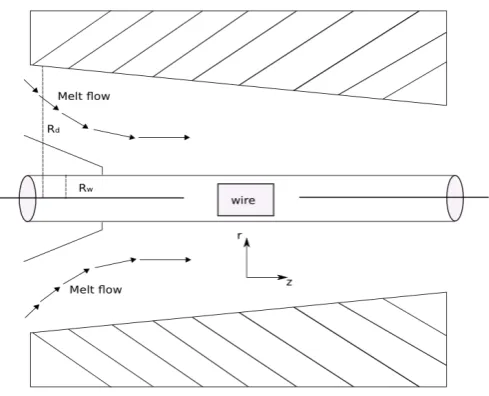
The principle of the flow geometry is schematically shown in figure 1. As shown in figure 1 the wire of radius is dragged with velocity through a pressure-type coating die of length and radius . The coordinate system is taken at the center of the wire, in which is taken perpendicular to the flow direction and −axis is along the flow. Here and represents the wire and die temperature respectively. A constant pressure gradient is acted upon the fluid direction and magnetic field of strength transversely along the axial direction. Due to small magnetic Reynold number the induced magnetic field is negligible, which is also a valid assumption on a laboratory scale.
The design of the coating die is more important because it affects the final product quality. In the current study, a pressurized coating die is considered. The impact of surrounding temperature is considered for optimal performance.
The coating die is filled with an elastic-viscous fluid. The flow is considered incompressible, laminar, axisymmetric and steady.
Figure 1. Pressure type coating die for wire coating analysis.
With the assumptions mentioned above, the velocity of the fluid, stress tensor and temperature field are taken as
( )
( )
0, 0, , , ( )
u= w r S S= r Θ = Θ r (1)
Subject to the boundary conditions
at w and 0 at d
w V= r R= w= r R= at r = Rw (2)
at
and
at
.
w
r R
w dr R
dΘ = Θ
=
Θ = Θ
=
(3)For an elastic-viscous fluid, the stress tensor is:
(
)
( )
(
)
3 5 6
1 2 1 1 2 1 2 1
D tr tr
Dt
γ γ γ
+ γ S+ + + +
S A S SA S A SA I
( )
2 7 2
1
1 2 4 1 2 1 ,
D
tr Dt
η γ
= + γ + γ +
A
A A A I
(4)
In the above
η
is the viscosity of the fluid,D
Dt
the material derivative,S
the extra stress tensor,1
1
,
TA
=
L
+
L L
= ∇
u
(5)1
1 1
,
2,3,...
T n
n n n
DA
A
A L
LA
n
Dt
−− −
=
+
+
=
(6)In the above equation denotes the transpose of the matrix.
It should be noted that the model (4) contains several other models as:
• For Newtonian fluid model all
γ − γ =
1 70
.• For second grade fluid model all
γ
1=
γ
3=
γ
5=
γ =
6γ =
70
.• For Oldroyd-B model all
γ − γ =
3 70.
• For Maxwell model all
γ − γ =
2 70
.• For Johnson-Segalman model all
γ
5=
γ
6= γ =
70.
• For Oldroyd 6-model all
γ = γ =
6 70.
The basic governing equations for incompressible flow are the continuity, momentum and energy equations are given by:
.
u
0,
∇ =
(7).T J B,
Du
Dt
ρ
= ∇ + ×
(8)2
T.L,
pD
c
k
Dt
ρ
Θ =
∇ Θ
+
(9)
In the above equationsu,
ρ
,T
, cp,D Dt
/
,k
,Θ
, are the velocity of the fluid, density of the fluid, shear stress,specific heat, material derivative, thermal conductivity, temperature and velocity gradient respectively.The interaction of current and magnetic field produces a body force
J B
×
as given in Eq. (8). The electrostatic force produced due to charge density is negligible and we only consider the applied magnetic fieldB
0 normal to the flow direction.In the above frame of reference the body force becomes.
2 0 .
J B = −
σ
B w (10)From Eqs. (1) and (8-10)the velocity and temperature fields are become:
(
)
3 2 4 22 2 2 2
2 2 2
3
2d w dw
dw
dw
d w
dw
d w
dw
d w
r
r
r
r
dr
dr
α β
dr
β
dr
dr
αβ
dr
dr
α
dr
dr
+
+
+
−
+
+
+
2
5 2 2
0
1
0,
B
dw
dw
w
dr
dr
σ
αβ
β
η
−
+
=
(11)
1
0,
rz
d
d
dw
k
r
S
r dr
dr
dr
Θ
+
=
where
(
) (
)(
)
5 71 4 7 3 5 4 7 2 ,
2
α=γ γ +γ − γ +γ γ + γ −γ −γ γ
(
) (
) (
)
5 61 3 6 3 5 1 3 6 1 2 .
β =γ γ +γ − γ +γ γ γ + −γ γ −γ γ
Introducing the dimensionless parameters
2
2 2 2
* * * * 2 0
2 2
2
, , , , , 1, , .
( )
d w
w w w w d w d w
w
V
B R
r w V V V
r w M Br
R R R R k
R σ α β η α β δ η Θ − Θ
= = = = = = > Θ = =
Θ − Θ Θ − Θ
(13)
In the above equation
α
,β
are the material parameters,M
the magnetic parameter,δ
and the radii ratio andBr
is the Brinkman number.The system of Eq. (2), (3), (11) and (12) in dimensionless form are become
(
)
3 2 4 22 2 2
2 2 2
3
d w dw
dw
dw
d w
dw
d w
dw
r
r
r
r
dr
dr
α β
dr
β
dr
dr
αβ
dr
dr
α
dr
+
+
+
−
+
+
5 4 2
2
1
2
0,
dw
dw
dw
M
dr
dr
dr
αβ
−
+
β
+
β
=
(14)
( )
1
1
w
=
,
w
( )
δ
=
0,
(15)2 2 2
1
1
1
,
d
d
du
du
du
r
Br
r dr
dr
dr
dr
dr
Θ
+ β
+
+ α
(16)( )
1
0,
( )
δ
1
.
Θ
= Θ
=
(17)5. Solution of the Modeled Problem
To solve Equations (14)–(17), we apply the Adomian decomposition method [38–42]. The detail of the method is given in appendix, while the zero and first order solutions for the velocity field and temperature distributions are:
0
,
1
r
w
δ
δ
− +
=
− +
(18)0
1
,
1
r
δ
+
Θ
=
−
− +
(19)(
)
2 2 3 2 2 2 2 2 2
2 2 2 2 2 3 2 2
2 2 2 2 2 2 2 2
2 2 2 2 3 2 2 2 2 2
1 5
3 3 3 9 3 9 3 3
6 3 4 3 3 6 3 9
3 6 6 15 3 3 6 12
1
12 6 6 3 3 6
6 1
M r M r r r r M r r M r r r
M M r M r M r r r M
r M r r M r r M M r
w M r M r r r
α α β β β β αβ αβ δ δ δ δ αδ αδ αδ βδ βδ βδ βδ βδ βδ αβδ αβδ δ δ δ δ αδ αδ αδ β δ − + + − + − − + − + + + − − − − + − + − + + − + − − − + = + + − − + − +
2 2 2 2
2 2 2 2 2 2 2 2 3 2 3 2 2 3 2 3 3
3 3 3 2 3 3 2 3 2 4 2 4
2 2 4 2 3 4 2 5 2 5 2 2 5 2 6 2 6
15 3 ,
9 3 6 14 8 18 4
3 3 3 6 3 6 16 3
12 9 6 3 2 2
M r
M r r M r M M r M r M r
r M r M r M M r
M r M r M M r M r M M r
( )
2 2 2 2 2
2 2 3 3
1 4 2 3
2 2 3 3
2 2
2 ln 2 ln 6 ln 2 ln
1 .
6 ln 2 ln 2 ln 2 ln 2 ln
2 1
2 ln 4 ln 4 ln 2 ln 2 ln
rR r R rR r R R rR r R R rR R rR r R R rR r r r r r r r r
r r r r r
r r r
α α δ δ δ αδ αδ δ δ δ δ δ β δ βδ δ δ δ δ δ δ βδ δ δ βδ δ δ δ δ δ δ δ δ δ − + − + + + − + − − + + + − − − + + − = + + − + − − + Θ − + + −
(21)
The second component is too large, so we only give the graphical representation upto the second order approximation.
Collecting the results, we have the velocity field and temperature distribution up to a first order approximation obtained by ADM as follows:
(
)
2 2 3 2 2 2 2 2 2
2 2 2 2 2 3 2 2
2 2 2 2 2 2 2 2
2 2 2 2 3 2 2 2
5
3 3 3 9 3 9 3 3
6 3 4 3 3 6 3 9
3 6 6 15 3 3 6 12
1
12 6 6 3 3
1 6 1
M r M r r r r M r r M r r r
M M r M r M r r r M
r M r r M r r M M r
r
w M r M r r
α α β β β β αβ αβ δ δ δ δ αδ αδ αδ βδ βδ βδ βδ βδ βδ αβδ αβδ δ δ δ δ δ αδ αδ δ δ − + + − + − − + − + + + − − − − + − + − + + − + − − − + − + = + + + − − − + − +
2 2 2 2 2 2
2 2 2 2 2 2 2 2 3 2 3 2 2 3 2 3 3
3 3 3 2 3 3 2 3 2 4 2 4
2 2 4 2 3 4 2 5 2 5 2 2 5 2 6 2 6
6 15 3
9 3 6 14 8 18 4
3 3 3 6 3 6 16 3
12 9 6 3 2 2
r M r
M r r M r M M r M r M r
r M r M r M M r
M r M r M M r M r M M r
αδ βδ βδ βδ βδ βδ βδ δ δ δ δ αδ αδ βδ βδ βδ βδ δ δ δ δ δ δ δ δ δ + − − + − + + + − − − + − + + − − + + + + − − − + (22) ( )
2 2 2 2 2
2 2 3 3
4 2 3
2 2 3 3
2 2
2 ln 2 ln 6 ln 2 ln
1 .
1 2 1 6 ln 2 ln 2 ln 2 ln 2 ln
2 ln 4 ln 4 ln 2 ln 2 ln
rR r R rR r R R rR r R R rR R rR r R R rR r r r r r r r r r
r r r r r
r r r
α α δ δ δ αδ αδ δ δ δ δ δ β δ βδ δ δ δ δ δ δ δ δ δ βδ δ βδ δ δ δ δ δ δ δ δ δ − + − + + + − + − − + + + − − − + + − − + = + − + − + + + − + − − + + − Θ (23)
6. Analysis of the Results
The subject of this section is to explore the effect of different emerging parameters such as
non-Newtonian parameters
α
andβ
, magnetic parameterM
and the Brinkman numberBr
on solutions(velocity and temperature profiles) are discussed through several graphs. The convergence of the method and comparison with published results is also established in this section.
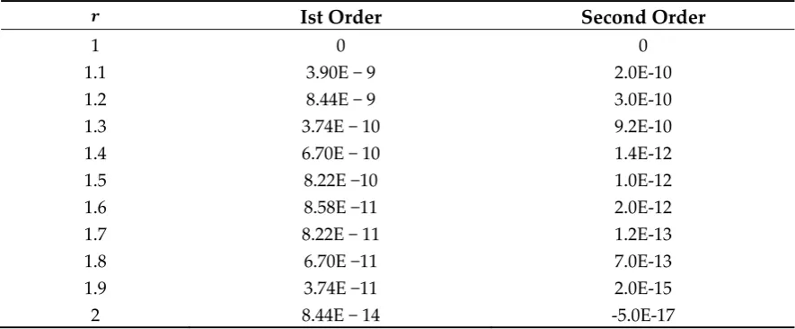
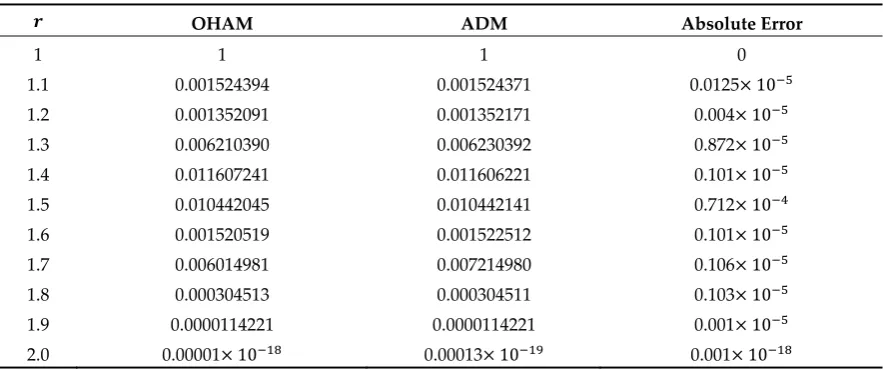
The convergence of the method is also necessary to check the reliability of the methodology. The convergence of the method is given in Tables 1–3 by assigning numerical values to the physical parameters of interest given in the appendix-D. From this we concluded that for different values of material parameters we get the convergence of the series solutions. The convergence of method can also be observed from the relative error of OHAM and ADM as given in the appendix-D in Table 4. Further, Table 5 in appendix-D also shows the comparison of present and published work by taking the magnetic parameter tends to zero and good agreement is found between the present and published work.
To give a clear overview of the physical problem, Figures 2–8 are sketched.
The impact of magnetic parameter
M
on the velocity profile is displayed in Figure 2. It is observed that the velocity profile decreases via largerM
. Physically by increasing the magnetic parameter the Lorentz force increases. Much resistance is occurring in the motion of the fluid which reduces the velocity of the fluid. The effect of magnetic parametersM
and the material parameterFigure2. Velocity profile for various values of
M
whenα
=
0.3,
β
=
0.2,
δ
=
2.
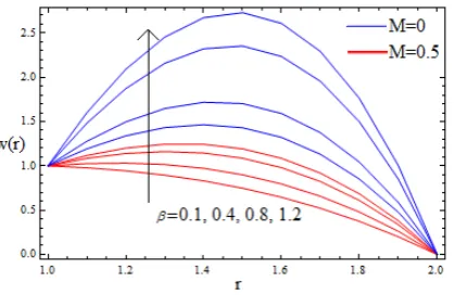
Figure 3. Velocity profile for various values of
β
whenα
=
0.3,
δ
=
2,
M
=
0.1.
Figure 4. Velocity profile for various values of when
β
=
0.3,
δ
=
2,
M
=
0.1.
is a resistive force and consequently enhance the temperature profile in the middle of the annular zone.
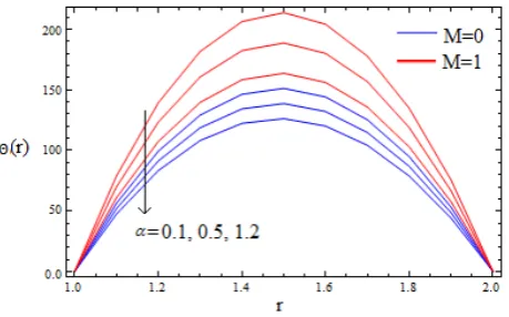
The effect of material parameter
α
and the non-Newtonian parameterβ
on the temperature profiles is shown in Figure 7 and 8 in the presence and absence of magnetic field, respectively. It is observed that the material parameterα
decreases the temperature profile while the non-Newtonian parameterβ
accelerates the temperature profile significantly, both in the presence and absence of magnetic field, at all the points of the melt polymer so as to make the process faster.Figure 5. Temperature profile for various of
M
whenα
=
0.3,
β
=
0.2,
δ
=
2.
Figure 6. Temperature profile for various of
Br
whenα =
0.4,
β
=
0.2,
M
=
0.2,
δ
=
2.
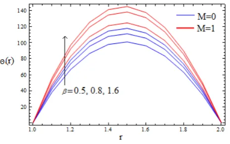
Figure 8. Temperature profile for various of
β
whenα =
0.3,
M
=
0.2,
δ
=
2.
5. Conclusion
In this work, the wire coating analysis and the heat transport phenomena corresponding to the steady flow has been studied. The fluid is electrically conducted in the presence of applied magnetic field. The problem is first modeled and then solved by utilizing ADM. The result is also verified by OHAM. Additionally, the convergence of the method is also verified. The effect of different emerging parameters on the solution is discussed. The material parameter
α
and the magnetic parameterM
have decelerated effect on the velocity profile. The velocity profile increases with increasingβ
. The temperature profile increases with increases magnetic parameterM
, Brinkman numberBr
and the material parameterβ
and decreases with increasingα
. At the end, the present is also compare with published results already available in the literature and good agreement is found.Author Contributions: Zesshan Khan and Rehan Ali Shah conceived and designed the simulated data; Saeed Islam and Bilal Jan analyzed the data; Haroon-Ur-Rasheed wrote the paper. I am very grateful to Dr. Aurangzeeb Khan, who gave me great help in the revised manuscript
Conflicts of Interest: The authors declare no conflict of interest.
Appendix A
Analysis of Adomian Decomposition Method (ADM)
The ADM is a steadfast method mainly used for the solution of nonlinear problems. One special area of application of this method is to solve equations arising when non-Newtonian fluids are studied. For better understanding we consider the following [38–41]:
( )
( )
0
,
n n
r w r
w ∞
=
=
(24)To find the components
w w w
0, 1,,
2,...,
w
n,separately, decomposition method is used.For this purpose we consider the following equation:
( )
( )
( )
( )
( )
,
t r
L
w
r
+
L
w
r
+
R
w
r
+
N
w r
=
g r
(25)( )
( )
( )
( )
( )
.
r t
Here
2
2 r
L
r
∂
=
∂
is linear operators,g r
( )
is the source term,Rw r
( )
is the remainder linearoperator and ( ) is a nonlinear term.
ApplyingL−r1on Eq. (26) to both sides, we have
( )
( )
( )
( )
( )
1 1 1 1 1
,
r r r r t r r
L L
−w
r
=
L g r
−−
L L
−w
r
−
L R
−w
r
−
L
−N
w
r
(27)
( )
( )
1( )
1( )
1( )
r t r r
r
f r
L L
r
L R
r
w
=
−
−w
−
−w
−
L N
−w
r
,
(28)
The function
f r
( )
,
arising fromL g r
−r1( )
,
after using the given boundary conditions. Theoperator
L
−r1=
∬
( )
. drdr
is used for second order differential equations.The series solution of
w r
( )
using ADM we have,( )
( )( )
1( )
1 n( )
0 0 0
,
n i r n r
n n n
w r
f
r
L R
w r
L N
w r
∞ ∞ ∞
− −
= = =
=
−
−
(29)In view of Adomian Polynomials the nonlinear term n
( )
0 nN
∞w r
=
in Eq. (29) can be expanded as( )
n0 0
,
n
n n
N
∞w r
∞= =
=
A
(30)In view of Eq. (29), Eq. (30) can expand as
( )
1(
)
1(
)
0 1 2 3 4 r 0 1 2 3 r 0 1
w
+ +
w w
+ + ……=
w
w
f r
−
L R
−w
+ +
w w
+ … −
w
L N
−A
+
A
+…
(31)
To determine the series components
w w w w
0, ,
1 2,
3…
, it should be noted that ADM suggest that( )
f r
in fact describe the zeroth componentw
0. The recursive relation is defined as:( )
( )
0
,
w r
=
f r
(32)( )
1( )
1( )
1r
L R
r 0r
r 0w
= −
−
w
−
L
−
A
,
(33)( )
1( )
1( )
2r
L R
r 1r
L
r 1,
w
= −
−
w
−
−
A
(34)( )
1( )
1( )
3r
L R
r 2r
r 2w
= −
−
w
−
L
−
A
.
(35)Appendix B
Analysis of Optimal Homotopy Asymptotic Method (OHAM)
The OHAM method is widely used by a number of researchers [42-45] for getting the approximate solution in series form. For better understanding consider the following equation in nonlinear form:
( ( )
( ))
( ) 0, ( ,
dw
),
L w r
Nw r
g r
B w
dr
+
+
=
(36)Where
L
is a linear operator,N
is nonlinear term,r R
∈
is independent variable,B
is boundary operator andg
is the source term. Similar to the analysis presented in [42-45] we construct the following set of equations for OHAM.[
1
]
[
( ) ( )
,
]
( ) ( ) ( )
[
,
( )
,
]
,
( ) ( )
,
,
,
=
0
,
∂
∂
+
+
−
+
−
r
p
r
p
r
B
p
r
N
r
g
p
r
L
p
H
r
g
p
r
L
p
ϕ
ϕ
ϕ
ϕ
ϕ
(37)Here
H p
( )
is the non-zero auxiliary function andϕ
( , )
r p
is a unknown function. Takingp
=
0
, the homotopy in Eq. (37) gives the zero component solution i.e.( )
( )
,
r
w
w
B
,
r
g
r
L
(
,
0
)
0
,
00
0
=
∂
∂
=
+
ϕ
(38)where the auxiliary function
H
( )
p
is taken as( )
p pC p C p C .,H = 1+ 2 2+ 3 3... (39)
C
C
C
1,
2,
3are auxiliary constants.
For estimated solution,
ϕ
( , )
r p
is expanding with respect top
by using Taylor series.0
1
( , , )
( )
( , , )
k, 1, 2,3...
i k i
k
r p C
w r
w r p C p
i
ϕ
∞=
=
+
=
(40)By using Eqs. (39) and (40) into Eq. (37), and equating the coefficient of like power of
p
, the zero order problem is given in Eq. (38). The first and second order problems are as follows:( )
(
) ( )
(
( )
)
( )
,
dr
r
w
d
w
B
,
r
w
N
C
r
g
r
w
L
,
10
1 0
0 1
1
=
=
+
(41)( )
(
)
(
( )
)
(
( )
)
[
(
( )
)
(
( )
)
]
( )
( )
, dx r w d r w B , r w N r w L C r w N C r w L r wL , 2 0
2 1 1 1 1 0 0 2 1
2 =
+ + = − (42) The general 1
1 0 0 1 0 1
1
( ( ))
k(
k( ))
k( ( ))
k i[ (
k i( ))
k( ( ), ( ),...,
i
L w r
L w
−r
C N w r
−C L w
−r
N
−w r w r
=
−
=
+
+
B( ,
k) 0, 2,3,...
k
dw
w
k
dr
=
=
Here
N
k−1( ( ), ( ),...,
w r w r
0 1w
k−1( ))
r
are the coefficient of i kp
−in expansion of
N
(
ϕ
( )
r
,
p
).
(
)
(
,
,
)
(
( )
)
(
0( ) ( )
,
1...
( )
)
..
1 1 0
0
i k i k m
i k
i
N
w
r
N
w
r
w
r
w
r
p
C
p
r
N
−− ∞
= −=
+
=
ϕ
(44)The convergence of Eq. (44) depends upon the auxiliary constant and order of the problem. If it converges at
p
=
1
,
one has:1 2 3 0 1 2 3
1
( , ,
,
,...
m)
( )
m i( , ,
,
,...
m).
i
w r C C C
C
w r
w r C C C
C
=
=
+
(45)In view of Eqs. (45) and Eq. (36) we have:
(
,
i)
(
(
,
i)
)
( )
(
(
,
i)
)
R r C
=
L w r C
+
g r
+
N w r C , i 1,2..m
=
(46)Many methods such as Ritz Method, Method of Least square, Collection and Galerkin’s method are used for the solution of auxiliary constants.
Here we use the Least square method to find the auxiliary constant [43-45]:
(
C
C
C
)
R
(
r
C
C
C
)
dr,
J
mb
a
m
,
,
,...
,...
,
2 1 22
1
=
(47)in the above equation and are constant values taking from the domain of the problem. The auxiliary constants
C
1,
C
2,...
C
m can be obtained from the following relation:.
0
...
1 1=
=
∂
∂
=
∂
∂
C
J
C
J
(48)
Finally, from the solutions of Eq. (36), the approximate solution is well-determined.
Many researchers such as Zeeshan [37, 41] and Marinca et al. [43-45] applied this method for solving highly nonlinear boundary value problem.
Appendix D
Table A1. Convergence of the method for
α
=
0.2,
β
=
0.1,
M
i=
0.01,
δ
=
2.
Ist Order Second Order
1 0 0
1.1 3.90E − 9 2.0E-10
1.2 8.44E − 9 3.0E-10
1.3 3.74E − 10 9.2E-10
1.4 6.70E − 10 1.4E-12
1.5 8.22E −10 1.0E-12
1.6 8.58E −11 2.0E-12
1.7 8.22E − 11 1.2E-13
1.8 6.70E −11 7.0E-13
1.9 3.74E −11 2.0E-15
Table A2. Convergence of the method for
α
=
0.3,
β
=
0.2,
M
i=
0.1,
δ
=
2.
Ist Order Second Order
1 0 0
1.1 7.51E-14 7.93E-16
1.2 2.77E-12 2.21E-14
1.3 1.73E-11 1.11E-13
1.4 5.02E-11 2.46E-13
1.5 9.34E-11 3.12E-13
1.6 1.28E-10 2.43E-13
1.7 1.39E-10 1.15E-13
1.8 1.23E-10 1.40E-14
1.9 -7.50E-11 1.97E-14
2 1.95E-11 2.26E-13
Table A3. Convergence of the method for
α
=
0.4,
β
=
0.3,
M
i=
0.2,
δ
=
2.
Ist Order Second Order
1 0 0
1.1 3E-11 2.64E-09
1.2 0 5.03E-09
1.3 -1E-10 6.92E-09
1.4 2E-10 8.14E-09
1.5 1.1E-09 8.55E-09
1.6 4.4E-09 8.14E-09
1.7 1.35E-08 6.92E-08
1.8 3.68E-08 5.03E-10
1.9 9.01E-08 2.64E-11
2 2.027E-07 -9.53E-13
Table A4. Numerical comparison of OHAM and ADM when
1 2 3 4
0.3, 0.001652328, 0.00173421, 0.0010243621, 0.0001825341
0.2, 2,M 0.1,C C C C .
β= α= δ = = = − = − = =
OHAM ADM Absolute Error
1 1 1 0
Table A5. Velocity comparison of the present work with published work [20] when
0.2,
0.1,
M
0.0,
2.
α
=
β
=
=
δ
=
OHAM [20] Absolute Error
1 1 1 0
1.1 0.0011703 0.0011712 0.0000009
1.2 0.0002104 0.0002125 0.0000021
1.3 0.0300722 0.0300710 0.0000012
1.4 0.0216071 0.0216012 0.0000059
1.5 0.0104212 0.0104221 0.0000009
1.6 0.0015412 0.0054533 0.0039121
1.7 0.0071200 0.0071401 0.0000201
1.8 0.0035020 0.0035013 0.0000007
1.9 0.0137500 0.0137521 0.0000021
2 0 0 0
References
1. Han, C.D.; Rao, D. The rheology of wire coating extrusion. Polym. Eng. Sci. 18 1019–1029 (1978). 2. Nayak, M.K. Wire coating analysis, 2nded., India Tech, New Delhi (2015).
3. Caswell, B.; Tanner, R.J.(Wire coating die using finite element methods.Polym. Eng. Sci., 18 417–4211978).. 4. Tucker, C.L. Computer Modeling for Polymer Processing. Hanser, Munich, 311–317(1989).
5. Akter,S. & Hashmi, M.S. J. Analysis of polymer flow in a canonical coating unit: power law approach, Prog. Org. Coat. 37 15–22 (1999).
6. Akter, S.; Hashmi, M. S. J. Plasto-hydrodynamic pressure distribution in a tepered geometry wire coating unit, in: Proceedings of the 14th Conference of the Irish manufacturing committee (IMC14), Dublin, 331– 340(1997).
7. Siddiqui,A.M., Haroon,T.; Khan, H. Wire coating extrusion in a Pressure-type Die in the flow of a third grade fluid, Int. J. of Non-linear Sci. and Numeric. Simul.10 247–257(2009).
8. Fenner, R.T.; Williams,J.G. Analytical methods of wire coating die design, Trans. Plast. Inst. (London), 35 701–706 (1967).
9. Shah, R.A., Islam, S., Siddiqui, A.M.; Haroon, T. Optimal homotopy asymptotic method solution of unsteady second grade fluid in wire coating analysis, J. Ksiam 15 201–222(2011).
10. Shah,R.A., Islam,S., Siddiqui,A.M.&Haroon, T. Exact solution of differential equation arising in the wire coating analysis of an unsteady second grad fluid, Math. And Comp. Mod. 57 1284–1288(2013).
11. Shah,R.A., Islam,S., Ellahi,M., Haroon,T.,Siddiqui,A.M. Analytical solutions for heat transfer flows of a third Grade fluid in case of post-treatment of wire coating, International Journal of the Physical Sciences, 64213–4223(2011).
12. Shah,R.A., Islam,S., Siddiqui,A.M.&Haroon. Heat transfer by laminar flow of an elastico-viscous fluid in post treatment analysis of wire coating with linearly varying temperature along the coated wire, Journal of Heat and Mass Transfer, 48903–914(2012).
13. Mitsoulis, E. Fluid flow and heat transfer in wire coating, Ad. Poly. Tech. 6467–487 (1986).
14. Oliveira,P.J.& Pinho, F.T. Analytical solution for fully developed channel and pipe flow of Phan-Thien, Tanner fluids, J. fluid Mech., 387271–280(1999).
15. Thien,N.P.& Tanner, R.I. A new constitutive equation derived from network theory, J. Non-Newtonian fluid Mech., 2 353–365(1977).
16. Kasajima,M. & Ito, K. Post-treatment of Polymer extrudate in wire coating. Appl. Polym. Symp., 20 221– 235(1973).
18. Bagley,E.B.& Storey, S.H. Wire and Wire Prod,381104–1122(1963).
19. Pinho, F.T.& Oliveira, P.J. Analysis of forced convection in pipes and channels with simplified Phan-Thien-Tanner fluid, Int. j. Heat Mass Transfer, 43 2273–2287 (2000).
20. R.A. Shah, S. Islam.,A.M. Siddiqui, T. Haroon, Wire coating analysis with Oldroyd 8-constant fluid by optimal homotopy asymptotic method, 63 (2012) 695–707.
21. Abel, S., Prasad, K.V.& Mahaboob,A. Buoyancy force and thermal radiation effects in MHD boundary layer viscoelastic fluid flow over continuously moving stretching surface. Int. J. Thermal Sci. 44 465–476 (2005). 22. Sarpakaya, T. Flow of non-Newtonian fluids in a magnetic field. AIChE Journal 7 324–328 (1961).
23. Abel, M.S., J.V.& Shinde, J.N. The effects of MHD flow and heat transfer for the UCM fluid over a stretching surface in presence of thermal radiation. Adv. Math. Phy. 2012, 21 (2015).
24. Chen, V.C. On the analytical solution of MHD flow and heat transfer for two types of viscoelastic fluid over a stretching sheet with energy dissipation, internal heat source and thermal radiation.Int. J. Heat Mass Transfer 19 4264–4273 (2010).
25. Akbar, N.S., Ebaid, A & Khan, Z.H. Numerical analysis of magnetic field effects on Eyring-Powell fluid flow towards a stretching sheet. J. Magn. Magn. Mater 382355–358 (2015).
26. Mabood, F., Khan, W.A.& Ismail, A.I. M. MHD boundary layer flow and heat transfer of nanofluids over a nonlinear stretching sheet.J. Magn. Magn. Mater 374 569–576 (2015).
27. Singh, V. & Agarwal, S. MHD flow and heat transfer for Maxwell fluid over an exponentially stretching sheet with variable thermal conductivity in porous medium. Int. J. Non-Linear Mech. 40 1220–1228 (2005). 28. Hayat, T. &Sajid, M. Homotopy analysis of MHD boundary layer flow of an upper-convected Maxwell
fluid. Int. J. Eng.Sci. 45 393–401 (2007).
29. Wang, Y. & Hayat, T. Fluctuating flow of a Maxwell fluid past a porous plate with variable suction, Nonlinear Analysis. Real World Applications 9 1269–1282 (2008).
30. Rashidi, S. & Dehghan, M. Study of stream wise transverse magnetic fluid flow with heat transfer around an obstacle embedded in a porous medium. J. Magn. Magn. Mater. 378, 128–137 (2015).
31. Ellahi, R., Rahman, S.U., Nadeem, S. & Vafai, K. The blood flow of Prandtl fluid through a tapered stenosed arteries in permeable walls with magnetic field. Commun. Theor. Phys. 63, 353–358 (2015).
32. Kandelousi, M.S.& Ellahi, R. Simulation of ferrofluid flow for magnetic drug targeting using the lattice Boltzmann method.Z.N. A. 70, 115–124 (2015).
33. Hayat,T., Khan,M. & Asghar,S. Homotopy analysis of MHD flows of an Oldroyd 8-contant fluid, ActaMechanica 168 (2004) 213–232.
34. Ellahi,R., Hayat,T., Mahmood,F.M.&Zeeshan, A. Exact solutions for flow of an oldroyd 8-contant fluid with non-linear slip conditions, Communication in Non-linear Science and Numerical Simulation, 15 (2009) 322– 330.
35. Bari,S.Flow of an Oldroyd 8-constant fluid in a convergent channel, ActaMechanica 148 (2001) 117–127. 36. Ellahi, R., Hayat,T., Javed,T. & Asghar,S. On the analytic solution of non-linear flow problem involving
Oldroyd 8-constant fluid, Mathematical and Computer Modeling, 48(2008) 1191–1200.
37. Zhu, T. and Wenjing, Y . Theoretical and Numerical Studies of Noncontinuum Gas-Phase Heat Conduction in Micro/Nano Devices. Numerical Heat Transfer, Part B: Fundamentals 57.3 (2010): 203-226.
38. Hongwei, Liu , Kun, X. u , Taishan Zhu , Wenjing, Y. e. Multiple temperature kinetic model and its applications to micro-scale gas flows. Computers & fluids 67 (2012): 115-122.
39. Adomian, G.A Review of the Decomposition Method and Some Recent Results for Non-Linear Equations, Math Comput. Model. 13 287–299(1992).
40. Wazwaz,A.M. Adomian Decomposition Method for a Reliable Treatment of the Bratu-Type Equations, Appl. Math. Comput. 166 652–663(2005).
41. Wazwaz,A.M. Adomian Decomposition Method for a Reliable Treatment of the Emden–Fowler Equation, Appl. Math. Comput. 161 543–560(2005).
42. Zeeshan, Islam, S., Shah, R.A., Khan, I. & Gul, T. & Gaskel, P. Double-layer Optical Fiber Coating Analysis by Withdrawal from a Bath of Oldroyd 8-constant Fluid, J. Appl. Environ. Biol. Sci., 5 36–51 (2015).
43.
Gul, T., Shah,R.A., Islam,S. & Arif,M.MHD Thin Film Flows of a Third Grade Fluid on a Vertical Belt With Slip Boundary Conditions, J Appl Math: Article ID 14: 707286 (2013).45. Marinca,V.,Herisanu. Application of Optimal Homotopy Asymptotic Method for solving non-linear equations arising in heat transfer, International communications in heat and mass transfer 35710–715(2008). 46. V. Marinca, V., Herisanu, N., Bota,C. & Marinca, B. An Optimal Homotopy Asymptotic Method applied to the steady flow of a fourth grade fluid past a porous plate. Applied Mathematics letters 22245–251(2009).
© 2017 by the authors; licensee Preprints, Basel, Switzerland. This article is an open access article distributed under the terms and conditions of the Creative Commons by
![Table A5. Velocity comparison of the present work with published work [20] when α=β==δ=](https://thumb-us.123doks.com/thumbv2/123dok_us/8015798.1332836/14.595.75.519.109.292/table-a-velocity-comparison-present-work-published-work.webp)
