A mathematical model for the COVID-19 outbreak and its applications.

A mathematical model for the COVID-19 outbreak

and its applications.

Roman Cherniha1,* and Vasyl’ Davydovych1

1 _{Institute of Mathematics, National Academy of Sciences of Ukraine, 3, Tereshchenkivs’ka Street, Kyiv 01601,}

Ukraine.

* Correspondence: [email protected]; Tel.: +380442352010

Abstract: A mathematical model is proposed for quantitative description of the outbreak of novel coronavirus COVID-19 Although the model is relatively simple, the comparison with the public data shows that an exact solution solution of the model (with the correctly-specified parameters) leads to the results, which are in good agreement with the measured data in China and Austria. Prediction of the total number of the COVID-19 cases is discussed and examples are presented using the measured data in Austria, France and Poland.

Keywords: nonlinear mathematical model; modeling infectious diseases; logistic equation; integrability; exact solution.

MSC:92D30, 34C11

1. Introduction

The outbreak of novel coronavirus called COVID-19 in China has attracted extensive attention of many scientists, in particular mathematicians working in mathematical modeling. The first papers were already published in February and March 2020 [1–7]. At the present time, the COVID-19 outbreak is already spread over the world as a pandemic. There were almost 4000000 coronavirus cases up to date May 8 [8]. This work is a natural continuation of [7], in which we used the measured data at the beginning of the pandemic.

At the present time, there are many mathematical models used to describe epidemic processes and they can be found in any book devoted to mathematical models in biology and medicine (see, e.g., [9–12] and papers cited therein). The paper [13] is one of the first papers in this direction. The authors created a model based on three ordinary differential equations (ODEs), which nowadays is called the SIR model. There are several generalizations of the SIR model and the SEIR model (see the pioneering works [14,15]), which involves four ODEs, is the most common among them. These two models are mostly used for numerical simulations in mathematical modeling the COVID-19 outbreak (see, e.g., [2,4,5]).

Our aim is to develop a simple mathematical model for the the COVID-19 outbreak, which possesses two properties, namely, one is integrable and one predicts results, which are relevant to the measured data. Of course, such kind of models cannot catch all features of this epidemic process, which is very complicated. However, the model provides good results without long and complicated numerical simulations. Moreover, it is possible to make some predictions with acceptable exactness.

The paper is organized as follows. In Sections2, we propose a simple model, which was developed using the public data about the COVID-19 outbreak presented by WORLDOMETER [8]. Then we generalize the model taking into account the known information that the mortality rate in several countries is rather high. Both model are based on nonlinear system of ODEs. We demonstrate that both models are exactly solvable.

In Sections3, we demonstrate that the model describes very good the COVID-19 outbreak in China. This case was used because there are obvious indications that this epidemic threat was effectively

removed in China. In Section4, the model is applied to the COVID-19 outbreak in Austria and Poland. It is shown that the rate of nonlinearity in the model varies from one country to another country. A prediction of the total number of the COVID-19 cases is also discussed and an example is presented using the measured data in Poland. We also discuss the applicability of the model to the COVID-19 outbreak in France, where the mortality rate is rather high.

Finally, non-trivial generalization of the model, which takes into account non-homogenous space distribution of the infected population and is based on an nonlinear PDE system, is suggested in Section5.

2. Mathematical model

The first nontrivial biological model used for calculation and the time evolution of the total world population of people was created in 1838 by Verhulst [16]. His model is usually called the logistic model and has the form (in dimensionless variables)

dU

dt =U(1−U), U(0) =N0>0,

and is the classical example in any textbook on Mathematical Biology. Its exact solution is well known

U(t) = N0e

t

1+N0(et−1)

and depending on the valueN0suggests three different scenarios for the population evolution. In

particular, the useful curve, the so-called sigmoid, is obtained ifN0<1/2 (see, e.g., Fig. 1.1 in [17]).

We have noted that the data [8] for the total number of the COVID-19 cases in China and some other countries can be approximated by a sigmoid with the correctly-specified parameters. Having this in mind, we introduce a smooth functionu(t), which presents the total number of the COVID-19 cases identified up to dayt(for any integer numbert). We assume that the first case (cases)u0was

(were) identified att=0. Obviously, the functionu(t)is non-decreasing. So, we obtain

du

dt =u(a−bu), u(0) =u0≥0 (1)

whereaandbare positive constants. One may defineaasa0S, wherea0<1 is the infection rate andS

is an average number of healthy persons, who was contacted by a fixed infected person (the so-called mechanism of the virus transmission). Obviously, each infected person can be in contact only with a limited number of people (usually it is relatives and close friends). The termbuhas an opposite meaning toa, because one reflects the effortsB, in order to avoid contacts with infected persons and to make other restrictions introduced by the government. The coefficientBshould increase with growing

u(t). In other words, the government and ordinary people should apply stronger measures in order to stop growingu(t), otherwise the control on the epidemic process will be lost. So, we assume that

B≈bu1+γ_{withγ>0, therefore the termbu}1+γ_{(hereb>0) leading to the equation} du

dt =u(a−bu

γ_{), u(0) =u}

0≥0 (2)

is derived. In the caseγ = 1, Eq. (2) coincides with (1). We note that the nonlinearity in (2) was introduced by Ayala, Gilpin and Ehrenfeldin in [18] for describing competition between species, while the logistic equation in epidemiology occurs naturally and it is shown under some general assumptions by Brauer in [9].

During the epidemic process there are two possibilities for the infected persons. A majority, say

w, among them will recover, while some people,v, will die. Obviously, the equality

takes place at any timet. A typical equation for the time evolution ofv(see the last equation in the SIR model) is

dv

dt =k(t)u, v(0) =v0≥0 (3)

(a similar equation can be written forwbut there is no need to use more equations), wherev0is the

number of deaths att=0. Here the coefficientk(t)>0 reflects the effectiveness of the health system of the country (or a region) in question. From mathematical point of view, this coefficient should have the asymptotic behaviork(t)→0, ift→∞, otherwise all infected people will die. In particular, the useful form isk(t) =k0exp(−αt),α>0.

Now we point out that the model (2)–(3) is constructed under essential simplifications of the epidemic process in question. In particular, the model implicitly admits thatu v, otherwise the right-hand-sides of the basic equations should involve the functionw. Although the model is relatively simple, the comparison with the public data shows that an exact solution of the model (with the correctly-specified parameters) leads to the results, which are in good agreement with the measured data (see Sections3and4).

On the other hand, it is well-known that the COVID-19 outbreak in several countries is so severe that the mortality rate is rather high, i.e. the assumptionuvis not true. For example,v≈0.14uin Italy andv≈0.15uin France [8] (up to date May 5, 2020). In such cases, the model (2)–(3) should be generalized as follows

du

dt = (u−v)(a−b(u−v)

γ_{), u(0) =u}

0≥0, (4)

dv

dt =k(t)(u−v), v(0) =v0≥0. (5)

In fact, the time evolution of the functionucannot depend on the infected persons who already died. Similarly, the number of new deaths cannot depend on the people who already died. Taking into account the equalityu−v=w, the model (4)–(5) is reducible to the form

dw

dt =w(a−k(t)−bw

γ_{), w(0) =w}

0=u0−v0≥0, (6) dv

dt =k(t)w, v(0) =v0≥0. (7)

Now we realize that the nonlinear equation in (6) is the known Bernoulli equation. Thus, solving the initial problem (6) and substitutingwinto (7), we arrive at the exact solution in the explicit form

w(t) =eat−

Rt

0 k(t)dt

w−₀γ+bγ

Z t

0 e γ

at−Rt

0 k(t)dt

dt −_γ1

, (8)

v(t) =v0+ Z t

0 k

(t)w(t)dt, (9)

u(t) =v0+w(t) + Z t

0 k

(t)w(t)dt. (10) Obviously the further calculations depend essentially on the form of the coefficientk(t). In particular, settingk(t) =k0exp(−αt),α>0 we obtain

w(t) =exp at+ k0

αe −αt

!

eγkα0w−γ 0 +bγ

Z t

0 exp

γat+γk0 α e

−αt

dt −1_γ

,

v(t) =v0+k0 Z t

0 e

u(t) =v0+w(t) +k0 Z t

0 e

−αt_w(t)dt.

In the subsequent sections we concentrate ourselves on the countries, in whichuvso that the simplified model (2)–(3) can be used. The general model will be discussed in Section5.

3. Application for the COVID-19 outbreak in China

The general solution of Eq. (1) is well-known, so that Eq. (3) with the given functionk(t)can be easily integrated. So, settingk(t) =k0exp(−αt),α>0, we arrive at the exact solution of the model (1) and (3)

u(t) = au0eat

a+bu0(eat−1),

v(t) =ak0u0R₀t e

(a−α)τ

a+bu0(eaτ−1)dτ+v0.

(11)

Remark 1. The integral in (11) leads to an expression involving the special function LerchPhi(y,c,ν) ≡ ∑∞n=0 y

n

(ν+n)c, which cannot be expressed in terms of elementary functions for arbitrary parametersαand a. However, it can be done in some specific cases. For example, one obtains

v(t) = 2k0

√ u0 p

b(a−bu0)

arctan

√ bu0 √

a−bu0 eat2

−arctan

√ bu0 √

a−bu0

+v0 in the case2α=a.

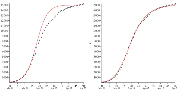
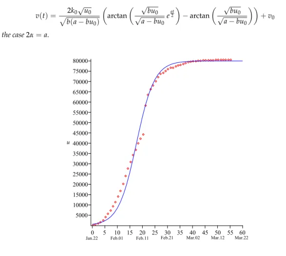
Figure 1. The comparison of the exact solutionu(t)(11) witha=0.28, b= _20000007 , u0=571 (blue curve) and the measured data of the COVID-19 cases (red dots).

u(t) =a1/γ_u

0eat a+buγ0(eaγt−1) !−1/γ

,

v(t) =a1/γ_k

0u0R₀te(a−α)τ a+bu₀γ(eaγτ−1) !−1/γ

dτ+v0.

(12)

Now we need to specify all the parameters in (11) using the data for the COVID-19 outbreak in China. We assume from the very beginning thatγ=1, i.e. the model (1) and (3) is applied. It follows from [8](here we use the official data presented by the government of China before April 17,2020) that the earliest well-founded data were fixed on Jan.22, hence we fix this date ast=0 and immediately obtainu0 =571 andv0 = 17. The parameterbcan be found from the known asymptotic behavior

of the functionu(t)in (11) and information from [8], thereforeb≈ ₈₀₀₀₀a . The plausible interval for parameteracan be estimated by using option ‘animation’ in MAPLE in order to fit plot of the function

u(t)to the measured data after Jan.22. So, we have numerically proved thata∈[0.25, 0.30].

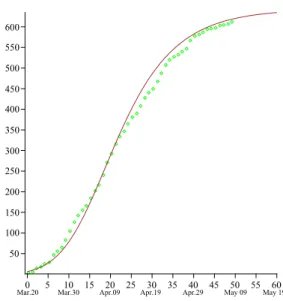
Figure 2.The comparison of the exact solutionv(t)(11) witha=0.28, b= _20000007 , u0 =571, k0= 0.0094, α=0.07, v0 =17 (brown curve) and the measured data the total number of deaths (green dots).

Because the functionv(t)should be monotonic non-decreasing function (we remind that it is the number of total deaths), we conclude thata>α. It was identified that a good choice is 4α=a. Finally, the coefficientk0was found from the formula

v

_t=T≡571k0 Z T

0

e0.21τ

1+₈₀₀₀₀571 (e0.28τ₋₁₎dτ+17=V

(hereVis the number of total deaths in the timet=Tpresented in [8]) for the fixed value ofa=0.28. The value of the coefficientk0is slowly varied from 0.0092385 to 0.0096878 ifTis changed from 65 to

Fig.1and Fig.2present the comparison of the results obtained from the model (1) and (3) (with the parameters specified above) and the measured data for the COVID-19 outbreak in China [8]. One may note that there is a good agreement between the total number of the COVID-19 cases and that predicted by our model. Of course, one may claim that exactness is not sufficiently good in the interval

t∈[10, 25]in Fig.1. However, we assume that either the method of measurement of the COVID-19 cases was corrected, or an unpredictable spike of such cases occurred around datet=25 (there is a jump from 44653 cases on Feb.11 to 58761 cases on Feb.12 [8]).

The comparison between the total number of deaths and that predicted by our model shows that exactness is sufficiently good for any time (see Fig.2). One may also note that the functionv(t)is still increasing beyond the timet=60. Such behavior reflects the real situation in the epidemic process, namely: some people will die even in absence of new COVID-19 cases because they were infected earlier. So, the final number of total deaths will be fixed later than that of the COVID-19 cases.

It should be noted that the parameterγplays essential role if one uses Eq. (2) instead of Eq. (1). In order to highlight this, we present exact solutions of Eq. (2) with different values ofγin Fig.3(all other parameters are the same as in Fig.1). One may see thatγ= 1 is a good choice in the case of China. On the other hand, taking into account the known data [8], we conclude thatγ<1 in the case of many other countries (the the next section).

Figure 3.The solutionu(t)of Eq. (2) forγ=0.3 (red curve),γ=0.5 (green curve),γ=1 (blue curve),

γ=1.5 (black curve) and the measured data of the COVID-19 cases in China(red dots).

4. Application for the COVID-19 outbreak in Austria and Poland

Figure 4. The comparison of the exact solutions (red curves)u(t) from (11) witha = 0.275, b = a

15000, u0 =104 (left) andu(t)from (12) withγ=2/5, a=0.383, b=₁₅₀₀₀a2/5, u0 =104 (right) and

the measured data of the COVID-19 cases inAustria(black dots).

Some well-known recommendations naturally follow from the model. It follows from the exact solution (11) that one needs to reduce the coefficienta=a0Sas much as possibly. It means that the

number of contactsSshould be minimized. On the other hand, the government should make more efforts (to close shops, restaurants, to restrict transport traffic etc.) in order to increase the function

B(u). These efforts should increase with growing of the total number of the COVID-19 cases. The government restrictions can be stopped only under condition that that the number of new COVID-19 cases per day already began to decrease from day to day. It means mathematically that the second order derivative of the functionu(t)takes negative values. In order to find the so-called critical number

u∗, we analyze the functionu(t)from (11). Calculating the second order derivative, one obtains

u00= u0a

3_(a−bu

0)eat a−bu0−bu0eat

(a−bu0+bu0eat)3

.

Solving the algebraic equationu00=0 with respect to the time, we arrive at

t∗= 1

aln

a bu0

−1

,

henceu∗=u(t∗). On the other hand, formulau00=0 allows to find the parameterbprovided the time

t∗is known from the measured data. Assuming thatais known one calculates

b= a

u0(eat∗+1)

. (13)

In the quite similar way, one can obtain the analogous formulae using the exact solution (12) of the model (2) and (3). These formulae have the form

t∗= 1

aγln

a bγuγ₀

− 1

γ

!

i.e.

b= a

Figure 5. The comparison of the exact solutions (brown curve)v(t)from (12) withγ = 2/5, a =

0.383, b= a

150002/5, u0=104, v0=6, k0 =0.0224, α=0.1 and the measured data of the COVID-19

cases inAustria(green dots).

Taking into account interpretation of the parameters, we believe that the parameteravaries not so much asband can be specified (at least estimated with a sufficient exactness) as follows. Obviously, the total number of the COVID-19 cases in the initial period of epidemic process can be approximated asu(t)≈u0eat(seeu(t)in (11) and (12) for small time). So, having the measured data in the initial

period, we may specify the parametera. It means that our model allows to predict the total numbers of the COVID-19 cases if the data fort∗andu∗are known.

Example 1. Let us consider, an example. It can be noted from the public data [8] that the COVID-19 outbreak in Austria had the maximum number of new daily cases on March 26. So,u∗ =6909. If we fix March 8 as the initial pointt=0, thent∗=18 andu0=104 (we think that there are essential errors

in measuring at the very beginning of the epidemic process, so that it is unreasonable to start from very small numbers ofu0).

Now we make approximation of the measured COVID-19 cases using the formulau(t)≈104eat

during the first 10 days. It can be estimated that the parametersa ∈ [0.26; 0.29] provides a good approximation. As follows from the public data [8], the total number of the COVID-19 cases in Austria reached 15 002 on April 23 (notably we predicted on April 8, that this number will be 13800 [7], i.e. the error is only 8 percent). After this date, the new daily cases numbers are very small (at maximum 0.5 percent of the total number) so that we conclude that the COVID-19 outbreak is over in Austria (of course, some number of infected people will still need medical treatment for several weeks). So, we may define thatumax =a/b≈15000. Now we assume that in this case the same model works as for China. So, using formula (13) the exact value of the parametersaandbwere specified and the relevant exact solution for the functionu(t)was compared with the public data. The result is presented in Fig.4 (left) and one realizes that exactness is not acceptable. We conclude thatγ6=1 should be taken in the model.

Assumingγ<1, we have done the analogous calculations using formula (14) for different values ofγ. As a result, the parameterγ=2/5 was found as one of the best choices. The result is presented in Fig.4(right) and now one may claim that the exact solution of the modelγ=2/5 fits to the real data very good. The total number of deathsv(t)can be also calculated using the second formula in (12 with correctly-specified parametersαandk0. The comparison with the measured data is presented in

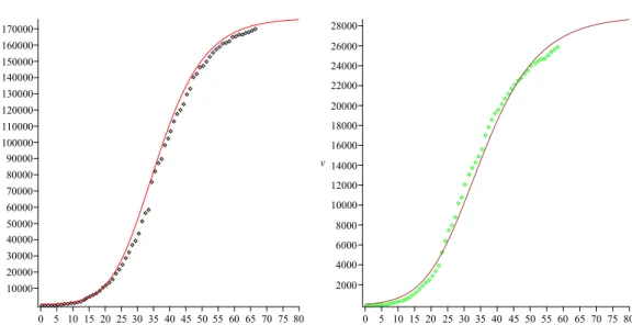
Figure 6.The comparison of the exact solutionu(t)(red curve) andv(t)(brown curve) from (12) with

γ=2/5, a=0.2835, u0=100, t∗=34, k0=0.02, α=0.036, v0=33 (parameterbis calculated by formula (14)) and the measured data of the COVID-19 cases (black dots) and the total number of deaths (green dots) inFrance.

Remark 2. It can be checked using the public data [8], that the exponentγ = 2/5is common for several

countries in Europe. See example, for France in Fig.6.

Example 2. Let us consider another example with the aim to make some predictions. It can be noted from the public data [8] that the COVID-19 outbreak in Poland is still dangerous. One may note that the maximum number of new daily cases occurred on April 19. So, we takeu∗=9287. If we fix March 14 as the initial pointt =0, thent∗ =36 andu0 =104. There are essential errors in

measuring at the very beginning of the epidemic process, so that it is unreasonable to start from very small numbers ofu0. Of course, one may take, say, March 12 or March 16 ast=0, however, it will be

shown below that the result will be almost the same.

So, making approximation of the measured coronavirus cases using the formulau(t) ≈ u0eat

at the initial stage of the COVID-19 outbreak, the interval for parametera∈[0.2; 0.3]was identified. Assuming that againγ=2/5 and using the formula (see (12))

u(t) =a5/2u0eat a+bu 2 5 0(e

2 5at−₁₎

!−5/2

, (15)

an analog of formula (13) can be easily derived. Now we may predict that the total number of the COVID-19 cases in Poland should beumax = (a/b)5/2≈19700. The relevant exact solution for the functionu(t)was compared with the public data and it was noted that a deviation occurs between our exact solution and the measured data.

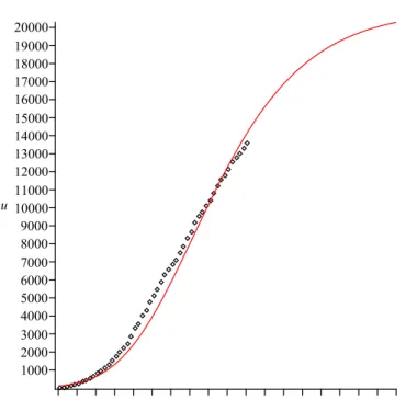
Figure 7.The comparison of the exact solutionu(t)from (12) (red curve) withγ=1/5,a=0.313, u0= 104, t∗=36 (parameterbis calculated by formula (14)) and the measured data of the COVID-19 cases inPoland(black dots).

Thus, the total number of the COVID-19 cases in Poland will be about 21000 (with the above listed exactness). This number will be reached in the middle of June 2020 and only 50–100 COVID-19 cases per day will be identified in the second half of June. Of course, if, for example, the Polish government will lift essentially the restrictions protecting the coronavirus spread too early thenumaxcan be much higher. On the other hand, if preliminary experimental data claiming that the COVID-19 virus die during a very short time under high temperature and sun light thenumax can be much smaller.

5. Discussion

In this work, we suggested to use the equations (2)–(3) as the mathematical model for describing the COVID-19 epidemic in several countries. Although it is not absolutely new model, one possesses two remarkable properties. Firstly, the model is integrable; secondly, one produces the results, which are relevant to the measured data in several countries. Moreover it can be done without long and complicated numerical simulations. Notably, we predicted on April 8 using the model, that the number COVID-19 cases in Austria will be 13800 [7], i.e. the error was less than 10 percent w.r.t. the measured data in the end of April.

We also developed a generalization of the model in the form (4)–(5). It is shown that this model is also exactly solvable and its exact solution is given by the formulae (8)–(10). We are going to apply this model to some countries with a hight mortality rate in a forthcoming paper.

Obviously, the model presented in this work cannot be thought as is applicable for the COVID-19 outbreak in each country. For example, the outbreak in China was mostly localized in the province Hubei. The size and population of this province are very small comparing with total those of China.

because the total number of deaths cases exceeds 14 percent of the total COVID-19 cases. In such cases, the natural generalization of the basic equations of our model reads as

∂u

∂t =d1∆(u−v) + (u−v)(a−b(u−v) γ_), ∂v

∂t =d2∆(u−v) +k(t)(u−v),

where∆is the Laplace operator,d1andd2are diffusivities, the functionsu(t,x,y)andv(t,x,y)are

analogs ofu(t)andv(t). Of course, the generalized model based on the system (15) and relevant boundary conditions (for example, zero flux conditions at the boundary) is much more complicated problem and cannot be solved analytically in contrast to the nonlinear models (2) – (3) and (4)–(5).

In the case of low mortality rate, i.e.uv, the above system simplifies to the form

∂u

∂t =d1∆u+u(a−bu γ_), ∂v

∂t =d2∆u+k(t)u,

(16)

Here we note that the first equation in (16) withγ=1 is the classical Fisher equation [19], which was extensively studied in many works (see, e.g., the monographs [11,20] and papers cited therein).

Notably, the system (16) can be essentially simplified under the reasonable assumptiond1=d2= dto the form (here wherew=u−v)

∂u

∂t =d∆u+u(a−bu γ_), ∂w

∂t =u(a−buγ)−k(t)u.

Conflicts of Interest:The authors declare no conflict of interest.

References

1. Luo, X.; Feng, Sh.; Yang J.; et al. Analysis of potential risk of COVID-19 infections in China based on a pairwise epidemic model.doi:10.20944/preprints202002.0398.v12020.

2. Peng, L.; Yang, W.;Zhang D.; et al. Epidemic analysis of COVID-19 in China by dynamical modeling. arXiv:2002.065632020.

3. Shao, N.; Zhong, M.; Yan, Y.; et al. Dynamic models for Coronavirus Disease 2019 and data analysis.Math. Meth. Appl. Sci.2020, 1–7.

4. Tian, J.; Wu, J.; Bao, Y.; et al. Modeling analysis of COVID-19 based on morbidity data in Anhui, China.MBE 2020,17, 2842–2852.

5. Efimov, D.; Ushirobira, U.; On interval prediction of COVID-19 development based on a SEIR epidemic model. [Research Report]Inria Lille Nord Europe - Laboratoire CRIStAL - Universite de Lille. hal-02517866v3 2020.

6. Weston, C.; Roda, W.; Varugheseb M.; et al. Why is it difficult to accurately predict the COVID-19 epidemic? Infectious Disease Modelling2020,5, 271–281.

7. Cherniha , R.; Davydovych, V.; A mathematical model for the COVID-19 outbreak. arXiv:2004.01487v2 2020.

8. https://www.worldometers.info/coronavirus

9. Brauer, F.; Castillo-Chavez, C.Mathematical models in population biology and epidemiology; Springer: New York, 2012.

10. Keeling, M.J.; Rohani, P.Modeling infectious diseases in humans and animals; Princeton University Press: Princeton, 2008.

11. Murray, J.D.Mathematical biology; Springer: Berlin, 1989.

12. Murray, J.D.Mathematical biology, II: Spatial models and biomedical applications; Springer: Berlin, 2003. 13. Kermack, W.O.; McKendrick, A.G. A contribution to the mathematical theory of epidemics. Proc. Roy. Soc.

14. Anderson, R.M.; May, R.M. Directly transmitted infectious diseases: Control by vaccination.Science1982, 215, 1053–1060.

15. Dietz, K. The incidence of infectious diseases under the influence of seasonal fluctuations; Lecture Notes in Biomathematics11, Springer: Berlin, 1976, pp. 1–15.

16. Verhulst, P.F. Notice sur la loi que la population suit dans son accroissement.Corr. Math. Physics.1838,10, 113.

17. Cherniha, R.; Davydovych, V.Nonlinear reaction-diffusion systems — conditional symmetry, exact solutions and their applications in biology; Lecture Notes in Mathematics2196, Springer: Cham, 2017.

18. Ayala, F.J.; Gilpin, M.E.; Ehrenfeld, J.G. Competition between species: Theorical models and experimental tests. Theoretical Pop. Biol.1973,4, 331–356.

19. Fisher, R.A. The wave of advance of advantageous genes. Ann. Eugenics.1937,7, 353–369.