Dimensionality reduction for parametric design exploration

Dimensionality

Reduction for

Parametric Design

Exploration

John Harding

J. Harding

Abstract

In architectural design, parametric models often include numeric parameters that can be adjusted during design exploration. The resulting design space can be easily displayed to the user if the number of parameters is low, for example, using a simple 2- or 3-dimensional plot. However, visualising the design space of models defined by multiple parameters is not straightforward. In this paper it is shown how dimensionality reduction can assist in this task whilst retain-ing associations between input designs at a high-dimensional parameter space. A self-organising map (SOM), a type of unsupervised artificial neural network, is used in combination with Rhino Grasshopper in order to demonstrate the potential benefits for design exploration.

Keywords:

1. Introduction

Dimensionality reduction (DR) is the study of reducing the number of variables that define any system. This is typically divided into two methods, feature selec-tion and feature extracselec-tion. For the former, the task involves selecting a subset of variables, typically those that have the greatest influence on the output. Fea-ture extraction, on the other hand, transforms the data into a new set of lower dimensional variables.

Techniques for feature extraction of high-dimensional data sets are well known in data-mining for both reducing storage space of complex data and vi-sualising high-dimensional data sets. Examples in speech (Kumar & Andreou 1998) and image recognition (Yu & Yang 2001; Hinton & Ruslan 2006) are now standard references in

pattern recognition, and research into using DR methods for solving engineering design problems (Bekasiewicz et al. 2014) is continuing at pace.

Dimensionality reduction has strong links to research in neuroscience and cognition, for example, in mapping sensory experience to associated three- dimensional locations in the brain, the so-called somatotopic map(Grodd et al. 2001). In AI research, some artificial neural networks attempt to artificially recreate this process by mapping complex inputs into a lower dimensional spaces, one

ex-ample being the SOM introduced by Kohonen (1982). This paper therefore

inves-tigates whether SOMs can be used effectively in combination with architectural parametric models defined by high-dimensional parameters.

2. Background

Visualising high-dimensional data for human cognition is hard. Examples with-out resorting to reducing dimensions include the use of colour on plots or by combining multiple plots representing different combinations of variables. Due to this mixed mode of representation, such diagrams can often be difficult to un-derstand and get an overall picture of the data set.

With feature extraction, reducing the high-dimensional data can be converted to a lower dimensional space. Feature extraction methods can be classified into two sets, linear and non-linear. Popular linear methods include K-means cluster analysis and principal component analysis (PCA). PCA, for example, transforms the data set to a lower dimensional orthogonal coordinate system that max- imises variance (Jolliffe 2002).

Whilst linear methods are often comparatively fast, they struggle to main-tain associations between data that is distributed non-linearly in the high-

dimensional space. A classic example is in handing the so-called Swiss-roll data

non-linear relationships include Sammon mapping (1969), Isomaps (Tenenbaum et al. 2001), elastic maps (Gorban & Zinovyev 2009), and SOMs (Kohonen 1982).

2.1 Precedents in Architectural Design

In architectural design, DR has been implemented predominantly in spatial anal-ysis. Coyne (1990) first used the idea of connectionism to display differences be-tween abstract residential plans. Petrovic and Svetel (1993) generated 3-dimensional

layouts based on higher dimensional semantic associations. More recent work

by Derix and Thum (2000) investigated a spatial machine that could build

autono-mous representations of space using SOMs. Methods for the classification of architectural plans have been investigated using both PCA (Hanna 2006; Hanna 2010) and

SOMs (Jupp & Gero 2006; Harding & Derix 2010). More recently, Derix and Jagannath (2014)

have used SOMs to capture and classify spatial descriptions.

Although these applications have shown the high potential of using DR methods in design, they are yet to have a wider impact in architectural comput-ing. This has in part motivated this research in returning to existing parametric modelling tools, offering new ways to enhance their use. The work presented here focusses on visualising parameter and not objective space (for example, performance criteria).

D

T

2.2 Potential for Parametric Models

A subset of parametric modelling tools based on dataflow programming asso-ciates input parameters and explicit functions to form a directed acyclic graph (DAG). The structure of the DAG typically describes a mapping of numbers into geometry, setting out a possible design space to be explored when parameters are adjusted (Aish & Woodbury 2005). Well-known examples of such DAG-based tools

used in architecture include Rhino Grasshopper (McNeel and Associates) and Autodesk Dynamo (Autodesk).

Visualising the design space of parametric models can help users to under-stand both the bounds of the model and how each parameter guides variation. For low-dimensional models, a simple plot is often sufficient to understand the

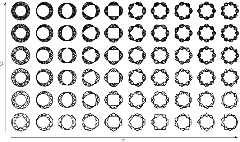
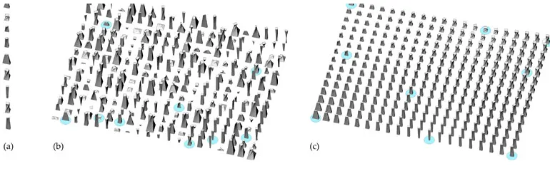
parameter space inherent in the model. Such an example is shown in Figure 1.

The design space of shapes defined by a set of parametric equations similar to Möbius bands is visualised. A parameter (T) governs a number of twists in the surface which is then discretised into a hexagonal pattern with increasing den-sity (D). In this particular case, it is possible to include semantic information to each parameter/axis, for example twist and density.

When models begin to increase in terms of independent variables (parame-ters), it becomes increasingly hard to understand the extent of the model. One is sometimes left adjusting different combinations of parameters and observing their effect on the output geometry. This is where DR techniques such as SOMs can potentially help visualise the bounds of a parametric model definition.

0.1 0.2 0.5 0.8 0.4 0.2 0.8 0.3 0.1 0.2 0.3 0.6 0.2 0.5 0.6 0.9 0.0 0.2 0.3 0.2 0.7 0.0 0.8 0.1 0.4 0.2 0.8 0.3 0.2 0.2 0.2 0.2 0.7 0.7 0.9 0.0 0.0 0.0 0.6 0.1 0.3 0.2 0.7 0.4 0.1 0.2 0.4 0.7 0.2 0.4 0.6 0.9 0.0 0.2 0.3 0.2 0.5 0.1 0.7 0.3 0.4 0.2 0.8 0.3 0.2 0.2 0.2 0.2 0.7 0.7 0.9 0.0 0.0 0.0 0.6 0.1 (a) (b)

3. Self-Organising Maps

SOMs are a type of unsupervised artificial neural network that can be used in reducing the dimensionality of data whilst attempting to retain non-linear

asso-ciations. Samples in the high-dimensional input feature space are presented to a

map in a lower dimensional map space, with the map learning over time from the

inputs presented to it.

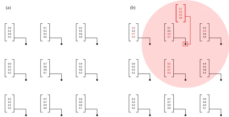
Typically, the map has either a hexagonal or rectangular topology arranged on a 2D plane, although this depends on the application. Each location in the

map has an associated feature vector (sometimes known as a synaptic vector) at

the same dimension as the input samples. In the example shown in Figure 2, a 2-

dimensional 3 x 3 map contains feature vectors in 4 dimensions. Before learning takes place, these feature vectors are typically randomised, meaning resulting maps for the same set of inputs, although similar, are never identical.

3.1 Learning

At each iteration, the inputs are presented to the map with the node with the closest feature vector to each input declared the winner. Determining this dis-tance can be done using various methods, including finding the Hamming disdis-tance (binary comparison) or simply taking the dot product for small input dimensions. The most common method, however, and that used here is to take the smallest

Euclidean distance (in feature space) to determine a winning node.

Once identified, a winning node adapts its feature vector slightly towards the input at a given rate (winner learning rate), with neighbouring nodes also learning depending on a radial function, typically a Gaussian radial basis function. These learning rates decay (exponentially) over time, with the map converging as learn-ing approaches zero. As the map changes, so the inputs move between winnlearn-ing nodes, making the SOM more than simply a form of high-dimensional diffusion.

The SOM algorithm has various parameters that govern the nature of learn-ing in the map. These include:

• Map dimension, size, and topology. • Winning node learning rate.

• Winning node learning decay rate.

• Neighbourhood learning function (e.g. Gaussian radial basis function). • Neighbourhood learning decay rate.

• Neighbourhood decay rate (affected neighbours shrinks over time).

discussed here, manual adjustment of the parameters were adequate to produce suitable maps for visualising parametric model design spaces. A more thorough

background to the SOM algorithm can be found in Kohonen (2001).

3.2 Reduction to 2D

The chosen map dimension can in theory be any equal or below the input space dimension. In this paper, 2-dimensional plots for the map were chosen in order

to best visualise the design space for human cognition. Figure 3 shows an

exam-ple of a 2-dimensional SOM on a rectangular grid being trained with five inputs. Each input is defined by a 3-dimensional vector corresponding to RGB values.

After 25 iterations learning has completed and the locations of the inputs on the map are distributed with similar colours being closer to each other and

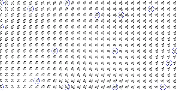
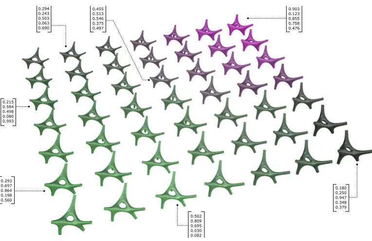
Figure 4. 9-dimesional ‘glyphs’ reduced to a two-dimensional map. The final 16 input locations are highlighted.

t = 0 t = 5 t = 25

those most different being furthest away. This associativity between inputs is maintained, despite a reduction from 3 dimensions to 2. As well as the input distribution, the map itself contains a smooth gradient between inputs, revealing colours that were not explicitly defined by the inputs.

Although non-linear DR can maintain associativity in the form of map re-gions, it is important to note that the original orthogonal structure of the data is lost. For example, one cannot associate axes to the sides of the 2-dimensional map, or in other words the mapping cannot be defined by a linear combina-tion of the three original variables. Another important aspect is that the whole visible spectrum as we know it is not shown; the map can only learn from the inputs presented to it.

Figure 4 shows a higher dimensional geometric example with sixteen random

9-dimensional input ‘glyphs’ being used to train a 2-dimensional map. Glyphs are similar to radar or spider plots in that each radial axis defines the value of a giv-en parameter. The resulting map produces a similar result to multi-dimgiv-ensional scaling (MDS) methods (Buja et al. 2008). In the example shown, in theory the nine

parameters could in theory control any aspect of a parametric model with the resulting geometry located at each map node.

4. Application in Parametric Design

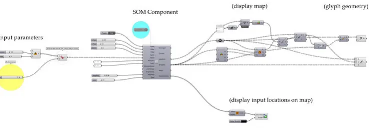
The use of DR methods in architectural design to date is relatively niche, so com-bining such techniques with popular parametric design software was the motiva-tion behind developing a tool for use in the architectural computing community. Written in C#, a freely available Grasshopper component was developed by the author for producing 2-dimensional SOMs with a rectangular topology (Harding 2016). The component consists of the control parameters as discussed in Section 3.2.

Figure 5 shows the use of the component to generate the glyph plot shown in Figure 4.

4.1 Parameter Encoding

In general, parametric design models map numbers to resulting geometry. The amount of indirectness in this mapping can vary, for example, a parameter that controls the height of a box can be seen as direct and linear – i.e. increasing the parameter also gradually increases the height of the output gradually. At the other end of the scale, parameters that are seeds for pseudorandom functions result in a completely indirect mapping between parameter and final geometry – a concept similar to that of continuous functions or smooth fitness landscapes in evolution.

Parametric models that use dataflow programming such as Rhino Grasshopper

do not typically allow cycles and therefore have a so-called explicit embryogeny

parameters are adjusted, and this usually helps in maintaining a direct mapping

between number and form. This is in contrast to chaotic (Lorenz 1963) or complex

systems such as class IV cellular automata (Wolfram 1986) that have a highly indirect mapping between parameter and resulting form.

So-called developmental encodings are generally more indirect than

paramet-ric models, for example, superformulas (Gielis 2003) and compositional

pattern-pro-ducing networks (CPPNs) (Stanley 2007; Clune & Lipson 2011) that vary graph topology. In

architectural design, Vierlinger (2015) has recently showed how such

developmen-tal encodings can help evolve neural networks that produce drawings in antici-pation of the user.

The nature of the mapping is therefore an important consideration when visualising a design space and will inevitably vary depending on the parametric definition. For example, if the parametric model is many-to-one, i.e. two values of a given parameter map to the same design (a periodic function, for example). In such cases, a method such as shape analysis (Costa & Marcondes 2000) is likely to be more appropriate for classifying geometry and forming a feature vector.

4.2 Sampling of Models

As with the examples given in Section 3.3, for high-dimensional parametric mod-els, a selection of samples (saved parameter states) selected at random from

the design space can be used to produce a lower-dimensional map. Figure 6 shows

a tower massing form defined by three parameters with a direct mapping that alter the twist, height, and tapering of a box. By using several inputs with nor-malised parameter values, the resulting 2-dimensional map can offer an overall visualisation of the design space inherent in the parametric model.

The spaces between the inputs are interpolated by the map itself. Again, note that we have lost the structure of the original 3 dimensions during the process,

i.e. no particular direction now indicates twist, density, or height, rather there

ex-ists regions in the map that have higher values of these parameters than others.

In this example, as the choice of inputs is random, there exists no prevalent structure or clustering in the high-dimensional space that requires maintaining. However, if particular designs (or parts of design space) are more desirable then these can be selected as the inputs to the map. As the specific sampling may vary, one must anticipate that linear methods may not be sufficient. Sampling such as the Swiss-roll data set (Tenenbaum et al. 2001) requires a non-linear method

to maintain high-dimensional clustering. This is discussed further in the next section.

4.3 Selective Sampling

If certain parameter combinations are preferred by the designer, then there exists a bias towards certain clusters in the data. These could be selected automatically using an objective function and/or selected artificially. Figure 7 shows the design

of a structural node as part of the UWE 2016 Research Pavilion. Each node is defined by five parameters, two controlling colour and three defining the mesh geometry. As opposed to random sampling, seven designs were selected from the parametric model by the design team by adjusting parameters in the tradi-tional way and saving parameter states.

The selected designs were then used as inputs in the SOM. The resulting map (Fig. 8) interpolates designs between the inputs as well as locating similar designs closer to each other on the map and dissimilar designs further apart. Again, although it is not possible to define linear axes on the map (as we could in 5-dimensional feature space), associations between designs are evident by viewing the map as a gestalt. The associative map gives an overview of the latent possibilities within the parametric definition. Without resorting to laborious slider

tweaking resulting in user fatigue (Piasecki & Hanna 2011), the map suggests possible design combinations that might have been otherwise missed.

4.4 Artificial Selection

Evolutionary algorithms with artificial selection often employ a visual interface

for engaging with the user. Dawkins’ biomorphs (1986), for example, involve

se-lecting designs which are then crossbred and mutated at each generation. Such

interactive evolutionary algorithms are known to be useful for exploring design

problems with no clearly defined goal. At each iteration, SOMs could potential-ly be used to display the design space to the user as part of a human-computer interactive process. In addition, associating a fitness landscape at this lower di-mensional parameter space could also potentially help better visualise the effect of parameters on different performance measures for different designs.

5. Conclusions

In this paper DR has been used in combination with a parametric modelling environment in order to visualise high-dimensional parameter spaces. As well as creating associations between inputs, the SOM can suggests possible de-sign avenues beyond that easily achieved by adjusting numeric parameters manually. Future research in linking parametric design with DR includes the following:

• The use of a hexagonal map topology which is known to improve the per-formance of the map (Länsiluoto 2004).

• Incorporating fitness plots in order to make comparisons between param-eter and objective space for architectural designs.

• Incorporate a form of sensitivity analysis to understand effect of param-eters on the final geometry (i.e. the directness of mapping from param- eters to design).

• Incorporating analysis measures as inputs to the map.

• Development of the SOM tool to generate 1- and 3-dimensonal maps. • Testing of complex parametric models where the ‘curse of dimensionality’

can make adequate sampling difficult.

Parameters:

B: blue colour index G: green colour index R: pipe radii

S: central node size (convex hull) D: mesh pipe density

R

S

D

Figure 7. Structural node joining six elements controlled by five parameters.

0.293 0.697 0.864 0.198 0.560

0.180 0.250 0.947 0.348 0.379 0.502

0.809 0.695 0.030 0.082

0.903 0.123 0.855 0.758 0.476

0.215 0.584 0.498 0.080 0.993

0.294 0.243 0.503 0.063 0.690

0.455 0.513 0.546 0.375 0.497

Acknowledgements

This work is part sponsored by the 2016/17 UWE VC Early Career Researcher Development Award.

References

Aish, Robert, and Robert Woodbury. 2005. “Multi-level interaction in parametric design.” In Smart Graphics, 151–162. Berlin Heidelberg: Springer.

Bekasiewicz, Adrian, Koziel Slawomir, and Zieniutycz Wlodzimierz. 2014. “Design Space Reduction for Expedited Multi- Objective Design Optimization of Antennas in Highly Dimensional Spaces.” In Solving Computationally Expensive Engineering Problems: Methods and Applications 97: 113–120.

Bentley, Peter J., and Sanjeev Kumar. 1999. “Three Ways to Grow Designs: A Comparison of Embryogenies for an Evolu-tionary Design Problem.” In GECCO, 99: 35–43.

Berglund, Erik, and Joaquin Sitte. 2006. “The Parameterless Self-Organizing Map Algorithm.” Neural Networks, IEEE Transactions 17, 2: 305–316.

Buja, Andreas, Deborah F. Swayne, Michael L. Littman, Nathaniel Dean, Heike Hofmann, and Lisha Chen. 2008. “Data Vi-sualization with Multidimensional Scaling.” Journal of Computational and Graphical Statistics, 17, 2: 444–472. Clune, Jeff, and Hod Lipson. 2011. “Evolving Three-Dimensional Objects with a Generative Encoding Inspired by

Develop-mental Biology.” In Proceedings of the European Conference on Artificial Life: 144–148.

Costa, Luciano da Fontoura Da, and Roberto Marcondes Cesar Jr. 2000. “Shape Analysis and Classification: Theory and Practice.” Boca Raton, Florida: CRC Press, Inc.

Coyne, Richard D., and A. G. Postmus. 1990. “Spatial Applications of Neural Networks In Computer-Aided Design.” Arti-ficial intelligence in Engineering 5, 1: 9–22.

Dawkins, Richard. 1986. “The Blind Watchmaker: Why the Evidence of Evolution Reveals a Universe Without Design.” New York: WW Norton and Company.

Deb, Kalyanmoy, Amrit Pratap, Sameer Agarwal, and T. A. M. T. Meyarivan. 2002. “A Fast and Elitist Multiobjective Genetic Algorithm: NSGA-II.” Evolutionary Computation, IEEE Transactions 6, 2: 182–197.

Derix, C., and P. Jagannath. 2014. “Near futures: Associative archetypes Architectural Design.” Wiley Online Library 84: 130–135.

Derix, C., and R. Thum. 2000. “Self-Organizing Space.” Proceedings of the Generative Arts Conference 3, Milan :1-10. Gielis, Johan. 2003. “A Generic Geometric Transformation That Unifies a Wide Range of Natural and Abstract Shapes.”

American Journal of Botany 90, 3: 333–338.

Grodd, Wolfgang, Ernst Hülsmann, Martin Lotze, Dirk Wildgruber, and Michael Erb. 2001. “Sensorimotor Mapping of the Human Cerebellum: fMRI Evidence of Somatotopic Organization.” Human Brain Mapping 13, 2: 55–73.

Harding, John, and Derix, Christian. 2011. “Associative Spatial Networks in Architectural Design: Artificial Cognition of Space Using Neural Networks with Spectral Graph Theory.” In Design Computing and Cognition ’10, edited by John S. Gero, 305–323. New York: Springer.

Harding, John. 2016. “A Self-Organising Map Component.” Accessed March 3, 2016. http:// http://www.grasshopper3d. com/profiles/blogs/self-organising-map

Hinton, Geoffrey E., and Ruslan Salakhutdinov. 2006. “Reducing the Dimensionality of Data with Neural Networks.” Science 313, 5786: 504–507.

Jolliffe, Ian. 2002. “Principal Component Analysis.” New York: Springer.

Jupp, Julie, and John S. Gero. 2006. “Visual Style: Qualitative and Context-Dependent Categorization.” AIE EDAM: Arti-ficial Intelligence for Engineering Design, Analysis, and Manufacturing 20, 3: 247–266.

Kohonen, Teuvo. 1982. “Self-Organized Formation of Topologically Correct Feature Maps.” Biological Cybernetics: 43, 1: 59–69.

Kohonen, Teuvo. 2000. “Self-Organizing Maps.” Berlin: Springer-Verlag.

Kumar, Nagendra, and Andreas G. Andreou. 1998. “Heteroscedastic Discriminant Analysis and Reduced Rank Hmms for Improved Speech Recognition.” Speech Communication 26, 4: 283–297.

Länsiluoto, Aapo. 2004. "Economic and Competitive Environment Analysis in the Formulation of Strategy: A Decision-Oriented Study Utilizing Self-Organizing Maps”. Turku: Publications of the Turku School of Economics and Business Administration. Lorenz, Edward N. 1963. “Deterministic Nonperiodic Flow.” Journal of the Atmospheric Sciences 20, 2: 130–141. Piasecki, M., and S. Hanna. 2011. “A Redefinition of the Paradox of Choice.” Design Computing and Cognition 2010 : 347–366. Sammon, John W. 1969. “A Nonlinear Mapping for Data Structure Analysis.” IEEE Transactions on Computers 5: 401–409. Stanley, Kenneth O. 2007. “Compositional Pattern Producing Networks: A Novel Abstraction of Development.” Genetic

Programming and Evolvable Machines 8, 2: 131–162.

Tenenbaum, Joshua B., Vin De Silva, and John C. Langford. 2000. “A Global Geometric Framework for Nonlinear Dimen-sionality Reduction.” Science 290, 5500: 2319-2323.

Vierlinger, Robert. 2015. "Towards AI Drawing Agents." In Modelling Behaviour: Design Modelling Symposium 2015, edit-ed by Mette Ramsgaard Thomsen, Martin Tamke, Christoph Gengnagel, Billie Faircloth, and Fabian Scheurer, 357–369. Switzerland: Springer International Publishing.

Yu, Hua, and Jie Yang. 2001. “A Direct LDA Algorithm for High-Dimensional Data – With Application to Face Recognition.”

Pattern recognition 34, 10: 2067–2070.