Simulation of three dimensional double-diffusive
throughflow in internally heated anisotropic porous
media
Abstract
A model for double-diffusive convection in an anisotropic porous layer with a constant throughflow is explored, with penetrative convection being simu-lated via an internal heat source. The validity of both the linear instability and global nonlinear energy stability thresholds are tested using three di-mensional simulation. Our results show that the linear threshold accurately predicts on the onset of instability in the steady state throughflow. However, the required time to arrive at the steady state increases significantly as the Rayleigh number tends to the linear threshold.
Keywords: Double-diffusive convection, Throughflow, Internal heat source, Finite differences, Anisotropic porous media
Nomenclature
(x1, x2, x3) = (x, y, z) Cartesian coordinates
v velocity
P pressure
T temperature
C concentration of salt
u dimensionless velocity
p dimensionless pressure
θ dimensionless temperature
φ dimensionless concentration of salt
µ viscosity
ε porosity
g gravitational acceleration
ρ density
ρ0 reference density
T0 reference temperature
C0 reference concentration
αt thermal expansion coefficient
αc solutal expansion coefficient
K(z) = K0s(z) permeability of the porous medium
K0 reference permeability
κt effective thermal diffusivity of the porous medium
κs thermal diffusivity of the solid component of the porous medium
κf thermal diffusivity of the fluid component of the porous medium
cp specific heat of the fluid at constant pressure
c specific heat of the solid at constant pressure
M ratio of heat capacities
Q (>0) internal heat source
RaL=R2t thermal Rayleigh number
R2
c solute Rayleigh number
Tf dimensionless form of the throughflow
a2 horizontal wavenumber, m2+n2
m, n dimensionless disturbance wave vector −
→ω = (ξ
1, ξ2, ξ3) vorticity vector
− →
ψ = (ψ1, ψ2, ψ3) potential vector
Lx box dimension in thex direction
Ly box dimension in they direction
1. Introduction
The literature on the study of the effect of vertical throughflow on convec-tive instability in a porous medium is much less widespread, although recent studies include Shivakumara and Suma [10], Shivakumara and Khalili [12], Shivakumara and Sureshkumar [13], Nield and Kuznetsov [14], Hill [15], Hill
et al. [16] and Capone et al. [17].
The effect of vertical throughflow on double-diffusive convection in a porous medium is important due to its applications in engineering (e.g. the directional solidification of concentrated alloys as well as in some energy storage devices) and geophysics (e.g. seabed hydrodynamics such as in hy-drothermal vent systems). The difficulty in dealing with such instability problems is that one has to solve time dependent equations with variable coefficients, and the work in this direction is very limited. Shivakumara and Nanjundappa [18] used linear stability theory to analytically investi-gate the effects of quadratic drag and vertical throughflow on double diffu-sive convection in a horizontal porous layer using the Forchheimer-extended Darcy equation. Shivakumara and Sureshkumar [19] investigated the effects of quadratic drag and vertical throughflow on the linear stability of a doubly diffusive Oldroyd-B-fluid-saturated horizontal porous layer. Altawallbeh et al. [20] analytically studied using both linear and weakly nonlinear stabil-ity analyses the double-diffusive convection in an anisotropic porous layer heated and salted from below with an internal heat source and Soret effect. Shivakumara and Khalili [11] studied the problem of double-diffusive con-vection in a fluid filled anisotropic porous layer. Hill et al. [21] studied this problem but with the presence of an internal heat source to allow penetrative convection to occur. In this paper, we explore the model presented in Hill
et al. [21] of double-diffusive throughflow in an internally heated anisotropic porous medium.
When the difference between the linear (which predicts instability) and nonlinear (which predicts stability) thresholds is very large, the validity of the linear instability threshold to capture the onset of the instability is unclear. Thus, we utilise the stability analysis of Hill et al. [21] to select regions of large subcritical instabiltiies and then develop a three dimensional simulation for the problem to test the validity of these thresholds. To achieve this we transform the problem into a velocity-vorticity formulation and utilise second order finite difference schemes. We use both implicit and explicit schemes to enforce the free divergence equation.
Standard indicial notation is used throughout the article, where (x1, x2, x3) =
2. Mathematical formulation and governing equations
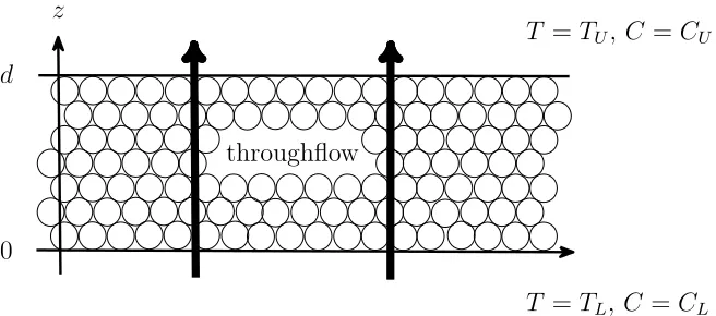
Utilising the approach of Hill et al. [21] (schematically shown in Figure 1) let us consider a layer Ω of a water saturated porous medium bounded by two horizontal planes. Let d > 0, Ω = R2×(0, d) and Oxyz be a cartesian frame of reference with unit vectors i, j, k.
d
0
z
T =TU, C =CU
T =TL, C =CL
[image:4.612.166.494.248.393.2]throughflow
Figure 1: Schematic representation of a cross-section of the system.
Assuming that the Oberbeck-Boussinesq approximation is valid (cf. [22] and references therein), the flow in the porous medium is governed by Darcy’s law
µ
K(z)vi =−P, i−kigρ(T, C), (1)
vi,i = 0, (2)
1
M T,t+viT, i=κt∇
2
T +Q, (3)
εC,t+viC, i=κc∇2C, (4)
We have denoted v, P, T, C, µ, ε, g and κc to be the velocity, pressure,
temperature, concentration of salt, viscosity, porosity, gravitational acceler-ation and salt diffusivity, respectively. The density ρ is of the form
ρ(T, C) = ρ0(1−αt(T −T0) +αc(C−C0))
where ρ0, T0 and C0 are a reference density, temperature and
concentra-tion, respectively, and αt and αc are the coefficients for thermal and solutal
expansion, respectively.
The permeability of the porous medium is taken to be of the form
K(z) =K0s(z),
whereK0is a reference permeability ands(z) = 1+λ1z/d,with constantλ1 >
−1 to ensure s(z) > 0. The effective thermal conductivity of the saturated porous medium κt is defined by the ratio between the thermal diffusivity of
the porous medium and the heat capacity per unit volume of the fluid:
κt=
(1−ε)κs+εκf
(ρ0cp)f
whereκsandκf are the thermal diffusivities of the solid and fluid components
of the porous medium, respectively and cp is the specific heat of the fluid at
constant pressure. The coefficient M is the ratio of heat capacities defined by
M = (ρ0cp)f
(ρ0c)m
. (5)
In (5) cis the specific heat of the solid, and
(ρ0c)m = (1−ε)(ρ0c)s+ε(ρ0cp)f,
denotes the overall heat capacity per unit volume of the porous medium. The subscripts f, s and m referring to the fluid, solid and porous components of the medium, respectively.
The Q (> 0) term in (3) is a (constant) internal heat source, with its inclusion allowing the model to describe penetrative convection in the porous layer [24].
CL > CU, so that the system is being salted from below. We allow for the
two cases of heating from below TL > TU and from above TL< TU.
Let us now consider the basic steady state solution of (1) – (4), with a throughflow in the z direction of the form
v= (0,0, V),
where V is constant. Utilising the boundary conditions, Eqs. (3) and (4) yield the temperature and concentration steady states
T(z) = Qz
V +TL+
V(TL−TU) +Qd
V(eV dκt −1)
(1−eV zκt),
C(z) =CL+
CL−CU
1−eV dκc
(eV zκc −1).
To investigate the stability of these solutions, we introduce perturbations
(ui, p, θ, φ) by
vi =ui+vi, P =p+P , T =θ+T , C =φ+C.
The perturbation equations are nondimensionalized according to the scales (stars denote dimensionless quantities)
p= µκt
K0
p∗, θ =θ∗
s
dQµ
gρ0αtK0
, xi =dx∗i, φ=φ
∗ s
µκt(CL−CU)
gρ0αcK0d
,
ui =
κt
du
∗
i, t=
d2
κtM
t∗, εb=M ε, Le= κt
κc
, Tf =
V d
κt
,
R2t = gρ0αtK0d
3Q
µκ2
t
, Rc2 = gρ0αcK0d(CL−CU)
µκt
, = (TL−TU)κt
Qd2 ,
whereR2t and R2c are the thermal and solute Rayleigh numbers, respectively, and Tf is the non-dimensional form of the throughflow. The dimensionless
perturbation equations are (after omitting all stars)
1
f(z)ui =−p, i+Rtθki−Rcφki, (6)
θ, t+uiθ, i+Tfθ,3 =Rtf1(z)w+∇2θ, (8)
b
ε φ, t+uiφ, i+Tfφ,3 =Rcf2(z)w+
1
Le∇
2φ, (9)
with w=u3 and f(z) = 1 +λ1z (with λ1 >−1 to ensure f(z)>0),
f1(z) =
Tf
eTf −1(+
1
Tf
)eTfz− 1
Tf
,
f2(z) =
Le TfeLeTfz
eLeTf −1 .
It is important to note that > 0 and < 0 correspond to heating from below and above, respectively. These equations hold in the region {z ∈ (0,1)} × {(x, y)∈R2} and the boundary conditions to be satisfied are:
u= 0, θ = 0, φ= 0, at z = 0,1, (10) where ui, p, θ and φ are assumed periodic in the x and y directions.
3. Linear and nonlinear energy stability theories
Linear instability results for stationary convection are obtained via the application of standard procedures to the linearized version of Eqs. (6)-(9). Following the approach of Hill et al. [21] the critical linear instability thresholds are located through the following eigenvalue problem for growth rate σ
f(D2 −a2)W −Df DW +a2Rtf2Θ−a2Rcf2φ= 0, (11)
(D2 −ζa2)Θ−TfDΘ +Rtf1(z)W =σΘ, (12)
1
Le(D
2−
a2)φ−TfDφ+Rcf2(z)W =bεσφ, (13)
on z ∈ (0,1). Here D = d/dz , w = W ei(mx+ny), θ = Θei(mx+ny), φ =
Φei(mx+ny) and a2 = m2 +n2 is a horizontal wavenumber. These equations arc subject to the boundary conditions
W = Θ = Φ = 0, at z = 0,1. (14)
predict the smallest instability threshold. It is possible that nonlinear terms will make a system become unstable long before the threshold predicted by linear theory is reached. Such instabilities are called subcritical. If we have a threshold below which we know all nonlinear perturbations decay, in a precise mathematical way, then this will yield a nonlinear stability boundary. When this threshold is relatively close to the analogous threshold of linear theory we can conclude that the linear results are actually predicting the physical picture correctly.
Hillet al. [21] developed an unconditional nonlinear energy stability the-ory for system (6)-(9) with the following eigenvalue problem:
f(D2−a2)W −Df DW +a2Rtf2(z)Θ−a2Rcf2(z)Φ = 0, (15)
2(D2 −a2)Θ +Rtf1(z)W +a2Rf(z)Ψ = 0, (16)
2λ
Le(D
2−a2)Φ +R
cλf2(z)W −a2Rcf(z)Ψ = 0, (17)
f2(D2−a2)Ψ +f Df DΨ +fΨD2f −(Df)2Ψ +Rtf2(z)f1(z)Θ
+λRcf2(z)f2(z)Φ = 0, (18)
with the boundary conditions
W = Θ = Φ = Ψ = 0, at z= 0,1, (19)
whereλis a parameter to be chosen and Φ is the normal mode representation of Lagrange multiplier (for more detail see [21]). The critical eigenvalue
RE(a2;λ) can be found from
RaE = max λ mina2 R
2
t(a
2;λ).
We solve the eigenvalue systems (11)-(13) for σ and (15)-(18) for Rt
numerically using three different numerical techniques to ensure accuracy, namely Chebyshev collocation [25], finite elements [26] and finite differences methods cf. [27]. The results are discussed in Section 6.
4. Velocity-vorticity formulation
the accuracy of the linear instability and nonlinear stability thresholds. A schematic diagram of the three-dimensional space (based on Figure 1) under consideration is given in Section 6.
Fasel [28] was the first article to address the velocity-vorticity form of the Navier-Stokes equations, and established this formula as an effective formulation for the solution of incompressible viscous flow problems. The velocity-vorticity form of the momentum equations is one of the best choices to achieve the divergence-free velocity field constraint for the incompressible Navier-Stokes equations in three dimensions. Moreover, the natural convec-tion problem can be simulated directly by the velocity-vorticity formulaconvec-tion, without the need to handle the pressure term. For the case of incompress-ible fluid flows, if the incompressibility condition imposed by the continuity equation is satisfied by some means, then a divergence-free flow field can be computed by solving the velocity-vorticity equations cf. Fasel [28], Napoli-tano and Catalano [29], Guj and Stella [30], Davis and Carpenter [31], Wong and Baker [32].
Mallinson and de Vahl Davis [33] first explored two dimensional natural convection in a rectangular box, with the proposition of the vorticity-stream function formulation without the pressure term. The problem of natural convection in a cubic enclosure has been studied using the velocity-vorticity equations by Wong and Baker [32]. However, there are two issues related with the velocity-vorticity formulation. Firstly, the number of variables is increased from four to six as compared to the primitive-variable form for three-dimensional problems. Secondly, it is not easy to enforce the vorticity definition at the solid boundaries to satisfy the continuity equation [34]. Davis and Carpenter [31] introduced a very important solution to the first problem, where only three governing equations were solved by considering two velocities and one vorticity as the primitive variables and computed the remaining three field variables as secondary variables. They handled the convective part of the governing equations using a predictor-corrector scheme, thus not deviating substantially from the existing algorithms for treating the pressure term. The solution of the second problem requires a higher-order scheme to compute the boundary vorticity values. Wong and Baker [32] introduced a second-order accurate Taylor’s series expansion to compute the vorticity values at the boundaries. Davis and Carpenter [31] used an integral approach for vorticity definition at the boundary, as followed by Guevremont et al. [35].
dif-ference schemes in the vorticity-vector potential formulation for computing the convective motion of an incompressible fluid in a porous material. The emphasis is on three dimensions and nonstaggered grids. We introduce a second-order accurate method based on the vorticity-vector potential for-mulation on the nonstaggered grid whose performance on uniform grids is comparable with the finite scheme. We will pay special attention to how accurately the divergence-free conditions for vorticity, velocity, and vector potential are satisfied. We will derive the three-dimensional analog of the local vorticity boundary conditions.
By using the curl operator to Eq. (6), one gets the following dimensionless form of the vorticity transport equation:
1
f(z)
−
→ω − f0(z)
f2(z)(−v, u,0) =R∇ ×θk−Rc∇ ×φk, (20)
where the vorticity vector −→ω = (ξ1, ξ2, ξ3) is defined as
−
→ω =∇ × −→v . (21)
To calculate velocity from vorticity, it is convenient to introduce a vector po-tential−→ψ = (ψ1, ψ2, ψ3),which may be looked upon as the three-dimensional
counterpart of two-dimensional stream function. The vector potential is de-fined by
−
→v =∇ ×−→ψ . (22)
It easy to show the existence of such a vector potential for a solenoidal vector field (∇ · −→v = 0), which is required to be solenoidal, i.e.,
∇ ·−→ψ = 0. (23)
Substituting Eq. (22) in Eq. (21) and using Eq. (23) yields
∇2−→ψ =−−→ω . (24)
The set of equations (8), (9), (20), (22) and (24) with appropriate boundary conditions form the basis for the numerical computations. The boundary conditions for the vector potential are given below
∂ψ1
ψ1 =
∂ψ2
∂y =ψ3 = 0, at y = 0,1, (26)
ψ1 =ψ2 =
∂ψ3
∂z = 0, at z = 0,1. (27)
The boundary conditions on vorticity follow directly and may expressed as
ξ1 = 0, ξ2 =−
∂w
∂x, ξ3 =
∂v
∂x, at x= 0,1, (28)
ξ1 =
∂w
∂y, ξ2 = 0, ξ3 =−
∂u
∂y, at y= 0,1, (29)
ξ1 =−
∂v
∂z, ξ2 =
∂u
∂z, ξ3 = 0, at z = 0,1. (30)
5. Numerical schemes
The first step in the numerical computational is to give an initial values for the vorticity vectorsξn
1ijk, ξ2nijk, ξ3nijk, i, j, k = 0,1, ..., m.Next, the Poisson
equation (24) is discretized in space using an implicit scheme as follows
(δx2+δy2+δz2)ψ1nijk+1 =−ξ1nijk, (31)
(δx2+δy2+δz2)ψ2nijk+1 =−ξ2nijk, (32)
(δx2+δy2+δz2)ψ3nijk+1 =−ξ3nijk, (33)
where δ2
x, δy2, δ2z are the second-order central difference operators, which are
defined as
δ2xφ= φi+1jk −2φijk+φi−1jk
(∆x)2 ,
δ2yφ = φijk+1−2φijk+φij−1k
(∆y)2 ,
δ2zφ = φijk+1−2φijk+φijk−1
(∆z)2 .
The Gauss-Seidel iteration method is utilised to evaluate ψ1nijk+1, ψ2nijk+1, ψ3nijk+1,
is to discretize Eqs.(25)-(27) to evaluate the ψ10n+1jk, ψ1nmjk+1 , ψ2ni+10k, ψ2nimk+1, ψ3nij+10,
ψn3ijm+1, i, j, k = 0, ..., m i.e. we used Eqs. (25)-(27) to evaluate the potential
vectors at the boundary. Now, the velocity vector can be calculated explicitly by using a second order finite difference scheme to Eq. (22) as follows:
uijkn+1 =δyψ3nijk+1−δzψ2nijk+1, (34)
vijkn+1 =δzψ1nijk+1−δxψn3ijk+1, (35)
uijkn+1 =δxψ2nijk+1−δyψ1nijk+1, (36)
i, j, k = 1, ..., m−1,
where δx, δy, δz are the first-order central difference operators, which are
de-fined as
δxφ=
φi+1jk−φi−1jk
2∆x ,
δyφ=
φij+1k−φij−1k
2∆y ,
δzφ=
φijk+1−φijk−1
2∆z .
The vorticity transport equation (20) is discretized in time using the explicit scheme. The discretized form of the vorticity transport equations (20) for the three vorticity components and energy equations (8) and (9) can be written as
1
fk
ξn1ijk+1 = f
0
k
f2
k
vijkn+1+Rδyθijkn+1−Rcδyφnijk+1
ξ2nijk+1 =−f
0
k
f2
k
unijk+1−Rδxθijkn+1+Rcδxφnijk+1
ξ3nijk+1 = 0, (37)
θijkn+1−θn
ijk
∆t +u
n
ijkδxθijkn +v n
ijkδyθnijk+w n ijkδzθijkn
+Tfδzθnijk =Rf1kwijkn + (δ
2
x+δ
2
y +δ
2
z)θ n
ijk, (38)
b
ε(φ
n+1
ijk −φnijk
∆t ) +u
n
ijkδxφnijk+v n
ijkδyφnijk+w n
ijkδzφnijk
+Tfδzφnijk =Rcf2kwijkn +
1
Le(δ
2
x+δ
2
y +δ
2
z)φ n
i, j, k = 1, ..., m−1.
The temperature on the boundary can be computed explicitly using Eqs. (10). However, a second order implicit technique has been used to evaluated the vorticity vector at the boundary form Eqs.(28)-(30). To enforce the vorticity definition at the wall, we used a Taylor’s series expansion to compute the vorticity values at the boundaries.
Here, we should mention that our scheme is flexible for variousRavalues and thus the grid resolution has been selected according to the Ra values. We decrease the values of ∆x, ∆y and ∆z as the value of Ra increases. However, for double-diffusive throughflow in porous media problem, we find that ∆x= ∆y= ∆z = 0.02 is enough to give us very accurate results.
6. Results and conclusions
To locate the stability thresholds, eigenvalue systems (11)-(13) and (15)-(18) have been solved using Chebyshev collocation, finite elements and finite differences methods.
In our use of the Chebyshev collocation method, we used between 20 and 30 polynomials. Usually 25 was found to be sufficient but convergence was checked by varying the number of polynomials and by examining the conver-gence of the associated eigenvector (which yields the approximate associated eigenfunction). For the finite elements method, we found that convergence to 8 decimal places is achieved with 3 elements, which each element having 11 nodes. For the finite differences scheme we found that convergence to 8 decimal places is achieved with h = 0.001. These techniques were selected due to their flexibility and accuracy cf. [25, 26, 27].
With respect to the physical system, instability refers to the destabiliza-tion of the steady state throughflow after a perturbadestabiliza-tion. If the flow returns to the steady state throughflow after a perturbation, this is stability. In this section, RaL, is the critical Rayleigh number for linear instability and RaE
is the global nonlinear stability threshold.
The corresponding critical wavenumbers of the linear instability and global nonlinear stability will be denoted by a2
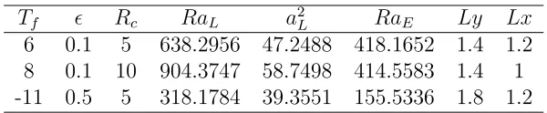
L and a2E. In Table 1, we present
in the z direction is always equal to 1. We assume that the perturba-tion fields (u, θ, π) are periodic in the x and y directions and denote by Ω = [0,2π/ax]×[0,2π/ay]×[0,1] to be the periodicity cell, where ax and
ay are the wavenumbers in the x and y directions, respectively. ax and ay
are evaluated according to the critical wavenumbers a2
L where a2L=a2x+a2y,
where Lx = 2π/ax and Ly = 2π/ay. The values of Lx and Ly in Table 1
may be rearranged to yield a number of possible solutions for each value of the critical wavenumbers. However, we select a solution so that these two values are similar to avoid any possible stabilisation effect from of walls.
We select the situations which have large subcritical regions, where the the linear threshold substantially different from the nonlinear one. This is a region of physical parameters for which the throughflow may potentially become unstable before the linear instability thresholds predicts it should.
To derive numerical solutions of the time dependent fully three dimen-sional problem, we use ∆t = 5×10⁻⁵ and ∆x = ∆y = ∆z = 0.02. The convergence criteria has been selected to make sure that the solutions arrive at a steady state. The convergence criteria is
ϕ= max
i,j,k{|ξ n+1 1ijk−ξ
n
1ijk|,|ξ n+1 2ijk−ξ
n
2ijk|,|ξ n+1 3ijk−ξ
n
3ijk|,|θ n+1
ijk −θ n ijk|},
and we select ϕ= 10−6. The program will continue computing the results of the temperature, velocity, vorticity and potential vector for new time levels until the results stratify the convergence criteria, otherwise, we stop the program after 80000 time levels, i.e at the time τ = 4.
To solve eqs. (31) – (33) using the Gauss-Seidel iteration method, in the first time level we give an initial value to the potential vector and we denoteψ11,kijk,ψ21,kijk,ψ13,kijk to be the potential vector. Then, using these initial values, we compute new values which we denote byψ11,kijk+1,ψ12,kijk+1,ψ31,kijk+1 and use these values to evaluate new values. The program will continue in this process until the convergence criteria is satisfied, which is
η = max
i,j,k{|ψ
1,k+1 1ijk −ψ
1,k
1ijk|,|ψ
1,k+1 2ijk −ψ
1,k
2ijk|,|ψ
1,k+1 3ijk −ψ
1,k
3ijk|}<10
−5.
In the next time levels, the values of ψ1ijk, ψ2ijk, ψ3ijk in the time level n
will be the initial values to the next time level.
Tf = 6, = 0.1, Rc = 10, R2 = 782, ∆t = 5×10⁻⁵,∆x = ∆y = ∆z =
0.02 . In Figure 2, the concentration, temperature and velocity contours are presented at the time level τ = 4 as the possibility of the solution arriving at the steady state is impossible due to the convergence criteria.
Figure 2 shows the contours of u, v, w, φ and θ in (a), (b), (c), (d), (e) and (f) respectively.
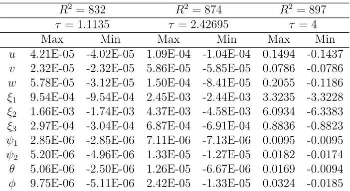
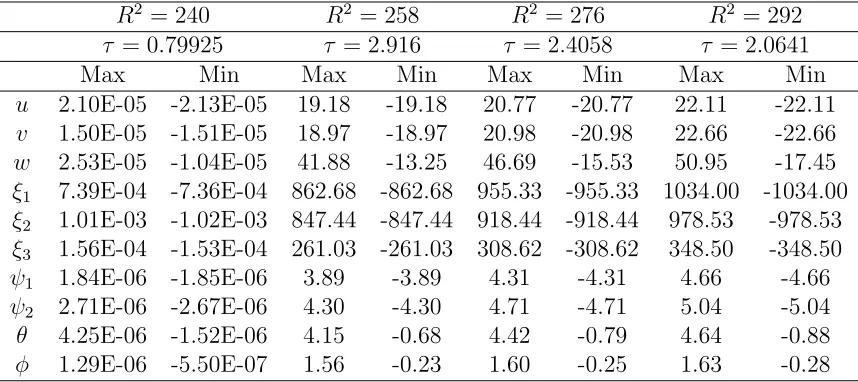
In Tables 2 – 4, we show a summary of the numerical results where we introduce the maximum and minimum values of temperature, velocity, vorticity and potential vectors. In Table 2, we select Tf = 6, = 0.1,
Le = 5, λ = 0.1 and Rc = 5, then according to the stability analysis we
have RaL = 638.2956, RaE = 418.1652, Lx = 1.4 and Ly = 1.2. Here, it
clear we have very large subcritical stability region as there is a big difference between the critical Rayleigh numbers of linear and nonlinear theories. From Table 2, for R2 = 588, we can see that the values of temperature, velocity,
vorticity and potential vectors satisfy the convergence criteria atτ = 1.25715 and thus the solution arrive to the basic steady state within a short time. However, for R2 = 625, the program needs τ = 3.34195 to arrive to the basic
steady state, which is expected as the the required time to arrive at a steady state increases with increasing R2 values until the solution does not arrive
at any steady state. Moreover, for R2 = 644, the solutions do not arrive at
any steady state and the program stops at τ = 4. For R2 = 644, we let the program work run for a significant period to test the convection’s long term behavior. We see that the values of the velocities increase at τ = 8, and then decrease at τ = 12 and continue in this oscillation. Here, according to the numerical results, the linear instability threshold is the actual threshold, i.e. the solutions arrive to the basic steady state before the linear instability threshold. However, the results of Tables 3 and 4 explain that the stability behavior is similar to the stability behavior of Table 2, as we found that the actual threshold is close to the linear instability threshold.
7. Conclusions
How-Tf Rc RaL a2L RaE Ly Lx
[image:16.612.155.455.123.185.2]6 0.1 5 638.2956 47.2488 418.1652 1.4 1.2 8 0.1 10 904.3747 58.7498 414.5583 1.4 1 -11 0.5 5 318.1784 39.3551 155.5336 1.8 1.2
Table 1: Critical Rayleigh and wavenumbersRaL, RaE, a2L at Le= 5 andλ= 0.1.
ever, the required time to arrive at the steady state increases significantly as the Rayleigh number tends to the linear threshold.
We find that the linear instability threshold (RaL) gives an accurate
pre-diction to the physical conditions under which the steady state throughflow will destabilise. If the Rayleigh number R2 is less than Ra
L, the
tempera-ture, velocity, vorticity and potential perturbations vanish, sending the so-lution back to the steady state, before the linear thresholds are reached. Numerically, the required time to arrive at the steady state increases as the value of R2 increases. When R2 is close to Ra
L, the solutions can tend
to a steady state which is different to the basic steady state v = (0,0, V).
When R2 > Ra
L the steady state throughflow destabilises, with oscillating
perturbations.
Finally, we can see that the stability results of the first two cases in Table 1 are different from the last one. The difference is that the position of the actual threshold. For the last case, it is really that the actual threshold is close to linear threshold but there is big difference between the actual and the linear thresholds. However, for the first two cases the actual threshold was very close to the critical Rayleigh number of linear theory. As we believe, this is because the system become more unsymmetric when Tf < 0 and
as the negativity value of Tf increase the actual threshold will be closer to
the critical Rayleigh number of the nonlinear theory. However, when the value of Tf is positive the system become more symmetric and thus the
actual threshold is close to the critical Rayleigh number of the linear theory. The effect of Tf connected with natural of the functions f1 and f2, where
R2 = 588 R2 = 625 R2 = 644
τ = 1.25715 τ = 3.34195 τ = 4
Max Min Max Min Max Min
u 4.62E-05 -4.48E-05 1.54E-04 -1.45E-04 0.5274 -0.4678
v 3.41E-05 -3.40E-05 1.06E-04 -1.06E-04 0.3233 -0.3233
w 6.87E-05 -2.29E-05 2.21E-04 -8.73E-05 0.7107 -0.3560
ξ1 1.57E-03 -1.56E-03 4.92E-03 -4.92E-03 15.2392 -15.2402
ξ2 2.05E-03 -2.12E-03 6.74E-03 -7.17E-03 22.0174 -24.6786
ξ3 2.17E-04 -2.24E-04 5.87E-04 -5.86E-04 2.4264 -2.4248
ψ1 4.40E-06 -4.42E-06 1.33E-05 -1.33E-05 0.0398 -0.0398
ψ2 6.00E-06 -5.84E-06 1.96E-05 -1.84E-05 0.0661 -0.0579
θ 6.48E-06 -1.82E-06 1.98E-05 -6.75E-06 0.0627 -0.0290
[image:17.612.123.489.141.333.2]φ 1.04E-05 -3.39E-06 3.16E-05 -1.22E-05 0.0980 -0.0496
Table 2: Summary of numerical results for Tf = 6, = 0.1, Le = 5, λ = 0.1, Rc = 5,
RaL= 638.2956,RaE = 418.1652,Lx= 1.4 andLy= 1.2.
R2 = 832 R2 = 874 R2 = 897
τ = 1.1135 τ = 2.42695 τ = 4
Max Min Max Min Max Min
u 4.21E-05 -4.02E-05 1.09E-04 -1.04E-04 0.1494 -0.1437
v 2.32E-05 -2.32E-05 5.86E-05 -5.85E-05 0.0786 -0.0786
w 5.78E-05 -3.12E-05 1.50E-04 -8.41E-05 0.2055 -0.1186
ξ1 9.54E-04 -9.54E-04 2.45E-03 -2.44E-03 3.3235 -3.3228
ξ2 1.66E-03 -1.74E-03 4.37E-03 -4.58E-03 6.0934 -6.3383
ξ3 2.97E-04 -3.04E-04 6.87E-04 -6.91E-04 0.8836 -0.8823
ψ1 2.85E-06 -2.85E-06 7.11E-06 -7.13E-06 0.0095 -0.0095
ψ2 5.20E-06 -4.96E-06 1.33E-05 -1.27E-05 0.0182 -0.0174
θ 5.06E-06 -2.50E-06 1.26E-05 -6.67E-06 0.0169 -0.0094
φ 9.75E-06 -5.11E-06 2.42E-05 -1.33E-05 0.0324 -0.0185
Table 3: Summary of numerical results for Tf = 8, = 0.1,Le = 5, λ= 0.1, Rc = 10,
[image:17.612.130.481.418.610.2]R2 = 240 R2 = 258 R2 = 276 R2 = 292
τ = 0.79925 τ = 2.916 τ = 2.4058 τ = 2.0641
Max Min Max Min Max Min Max Min
u 2.10E-05 -2.13E-05 19.18 -19.18 20.77 -20.77 22.11 -22.11
v 1.50E-05 -1.51E-05 18.97 -18.97 20.98 -20.98 22.66 -22.66
w 2.53E-05 -1.04E-05 41.88 -13.25 46.69 -15.53 50.95 -17.45
ξ1 7.39E-04 -7.36E-04 862.68 -862.68 955.33 -955.33 1034.00 -1034.00
ξ2 1.01E-03 -1.02E-03 847.44 -847.44 918.44 -918.44 978.53 -978.53
ξ3 1.56E-04 -1.53E-04 261.03 -261.03 308.62 -308.62 348.50 -348.50
ψ1 1.84E-06 -1.85E-06 3.89 -3.89 4.31 -4.31 4.66 -4.66
ψ2 2.71E-06 -2.67E-06 4.30 -4.30 4.71 -4.71 5.04 -5.04
θ 4.25E-06 -1.52E-06 4.15 -0.68 4.42 -0.79 4.64 -0.88
[image:18.612.112.541.126.317.2]φ 1.29E-06 -5.50E-07 1.56 -0.23 1.60 -0.25 1.63 -0.28
Table 4: Summary of numerical results for Tf =−11,= 0.5,Le= 5, λ= 0.1, Rc = 5,
RaL= 318.1784,RaE = 155.5336,Lx= 1.8 andLy= 1.2.
References
[1] S. K. Jena, S. K. Mahapatra, A. Sarkar, Double diffusive buoyancy op-posed natural convection in a porous cavity having partially active ver-tical walls, Int. J. Heat Mass Transfer 62 (2013) 808–817.
[2] S. K. Jena, S. K. Mahapatra, A. Sarkar, Thermosolutal Convection in a Rectangular Concentric Annulus: A Comprehensive Study, Transp. Porous Med. 98 (2013) 103–124.
[3] B. Chen, A. Cunningham, R. Ewing, R. Peralta, E. Visser, Two-dimensional modelling of microscale transport and biotransformation in porous media, Numerical Methods for PDEs 10 (1994) 65–83.
[4] B.J. Suchomel, B.M. Chen, M.B. Allen, Network model of flow, transport and biofilm effects in porous media, Transp. Porous Med. 30 (1998) 1–23.
[5] M.C. Curran, M.B. Allen, Parallel computing for solute transport models via alternating direction collocation. Adv. Water Res. 13 (1990) 70–75.
[7] F. Franchi, B. Straughan , A comparison of the GraC and Kazhikhov-Smagulov models for top heavy pollution instability, Adv. Water Res. 24 (2001) 585–594.
[8] A. Ludvigsen, E. Palm, R. McKibbin , Convective momentum and mass transport in porous sloping layers, J. Geophysical Res. 97 (2001) 12315– 12325.
[9] A. Gilman, J. Bear, The influence of free convection on soil salinization in arid regions, Transp. Porous Med. 23 (1996) 275–301.
[10] I.S. Shivakumara, S.P. Suma, Effects of throughflow and internal heat generation on the onset of convection in a fluid layer, Acta Mech. 140 (2000) 207–217.
[11] I.S. Shivakumara, A. Khalili, On the stability of double diffusive convec-tion in a porous layer with throughflow, Acta Mech. 152 (2001) 165–175.
[12] I.S. Shivakumara, A. Khalili, Non-Darcian effects on the onset of convec-tion in a porous layer with throughflow, Transp. Porous Med. 53 (2003) 245–63.
[13] I.S. Shivakumara, S. Sureshkumar, Convective instabilities in a viscoelastic-fluid-saturated porous medium with throughflow, J. Geo-phys. Eng. 4 (2007) 104–15.
[14] D.A. Nield, A.V. Kuznetsov, The effect of vertical throughflow on ther-mal instability in a porous medium layer saturated by a Nanofluid, Transp. Porous Med, 87 (2011) 765–775.
[15] A.A. Hill, Unconditional nonlinear stability for convection in a porous medium with vertical throughflow, Acta Mech. 193 (2007) 197–206.
[16] A.A. Hill, S. Rionero, B. Straughan, Global stability for penetrative convection with throughflow in a porous material, IMA J. App. Math. 72 (2007) 635–643.
[18] I.S. Shivakumara, C.E. Nanjundappa, Effects of quadratic drag and throughflow on double diffusive convection in a porous layer, Int. Com-mun. Heat Mass Transfer 33 (2006) 357–363.
[19] I.S. Shivakumara, S. Sureshkumar, Effects of throughflow and quadratic drag on the stability of a doubly diffusive Oldroyd-B fluid-saturated porous layer, J. Geophys. Eng. 5 (2008) 268–280.
[20] A.A. Altawallbeh, B.S. Bhadauria, I. Hashim, Linear and nonlinear double-diffusive convection in a saturated anisotropic porous layer with Soret effect and internal heat source, Int. J. Heat Mass Transfer 59 (2013) 103–111.
[21] F. Capone, M. Gentile, A.A. Hill, Double-diffusive penetrative convec-tion simulated via internal heating in an anisotropic porous layer with throughflow, Int. J. Heat Mass Transfer 45 (2011) 1622–1626.
[22] B. Straughan, The energy method, stability, and nonlinear convection, Applied Mathematical Sciences, second ed., vol. 91, Springer, 2004.
[23] D.A. Nield, A. Bejan, Convection in Porous Media, third ed., Springer-Verlag, New York, 2006.
[24] F. Capone, M. Gentile, A.A. Hill, Penetrative convection via internal heating in anisotropic porous media, Mech. Res. Com. 37 (2010) 441– 444.
[25] B. Straughan, A.J. Harfash, Instability in Poiseuille flow in a porous medium with slip boundary conditions, Microfluid Nanofluid, 15 (2013) 109–115.
[26] A.J. Harfash, Magnetic effect on instability and nonlinear stability of double diffusive convection in a reacting fluid, Contin. Mech. Thermo-dyn. 25 (2013) 89–106.
[27] A.J. Harfash, B. Straughan, Magnetic effect on instability and nonlinear stability in a reacting fluid, Meccanica. 47 (2012) 1849–1857.
[29] M. Napolitano, L. A. Catalano, A multigrid solver for the vorticity-velocity Navier-Stokes equations.Int. J. Numer. Meth. Fluids,13(1993) 49-59.
[30] G. Guj and F. Stella, A vorticity-velocity method for the numerical solution of 3D incompressible flows. J. Comput. Phys., 106 (1993) 286-298.
[31] C. Davis and P. W. Carpenter, A novel velocity-vorticity formulation of the Navier- Stokes equations with application to boundary layer distur-bance evolution. J. Comp. Phys., 172 (2001) 119-165.
[32] K. L. Wong and A. J. Baker, A 3D incompressible Navier-Stokes velocity-vorticity weak form finite element algorithm. Int. J. Numer. Meth. Fluids, 38 (2002) 99-123.
[33] G. D. Mallinson and G. de Vahl Davis, Three-dimensional natural con-vection in a box: a numerical study. J. Fluid Mech., 83 (1977) 1-31. [34] O. Daube, Resolution of the 2D Navier-Stokes equations in
velocity-vorticity form by means of an influence matrix technique. J. Comput. Phys., 103 (1992) 402-414.
-0.0050 -0.0050 0.16 -0.17 0.32 -0.33 0.16 0.48 -0.49 -0.17 0.64 -0.65 0.32 -0.33
0.0 0.5 1.0 1.5
0.0 0.5 1.0
y
x
(a)
2.8E-17 2.8E-17 -0.066 0.066 0.066 -0.066 -0.13 0.13 0.13 -0.13 0.066 -0.066 -0.20 0.20 0.20 -0.20 0.13 -0.13 -0.27 0.27 0.27 -0.27 -0.20 0.20
0.0 0.5 1.0 1.5
0.0 0.5 1.0
y
x
(b)
0.0075 0.14 -0.13 -0.13 0.28 -0.27 -0.27 0.42 -0.40 -0.40 0.55 -0.54 -0.54 0.14 0.14 0.14 0.14
0.0 0.5 1.0 1.5
0.0 0.5 1.0
y
x
(c)
-1.5E-06 -1.5E-06 -3.8E-06 -3.8E-06 -6.0E-06 -6.0E-06 -8.3E-06 -8.3E-06 -1.1E-05 -1.1E-05 -1.3E-05 -1.3E-05 -1.5E-05 -1.5E-05 -1.7E-05 -1.7E-05 -2.0E-05
0.0 0.5 1.0 1.5
0.0 0.5 1.0
y
x
(d)
-8.4E-04 -0.0017 -0.0025 -0.0034 -0.0042 -0.0051 -0.0059-0.0067 -0.0076
0.0 0.5 1.0 1.5
0.0 0.5 1.0
y
x
[image:22.612.125.526.133.638.2](e)
Figure 2: The contour maps atz= 0.5, Le= 5, λ= 0.1Tf = 6, = 0.1, Rc= 10, Lx= 1.8,Ly= 1.2, R2 = 782, ∆t= 5×10⁻⁵,∆x= ∆y = ∆z= 0.02. (a) u,(b)