CBCT IMAGE QUALITY ASSESSMENT TESTING CLINICALLY RELEVANT VOLUME ORIENTATION AND POSITION
Brittany L Kurzweg
A thesis submitted to the faculty at the University of North Carolina at Chapel Hill in partial fulfillment of the requirements for the degree of Masters of Science in the School of Dentistry
(Oral and Maxillofacial Radiology).
Chapel Hill 2017
© 2017 Brittany L Kurzweg ALL RIGHTS RESERVED
ABSTRACT
Brittany L Kurzweg: CBCT Image Quality Assessment Testing Clinically Relevant Volume Orientation and Position
(Under the direction of André Mol)
Introduction and Objectives: Some physical measures of CBCT image quality correlate well with diagnostic image quality. Traditionally, these measures have been assessed in the center in a standard orientation. The purpose of this study was to test whether measures of image quality vary as a function of test tool location, orientation and dose. The second purpose was to determine if there was an association between objective and subjective image quality.
Methods: CBCT objective image quality was assessed with one standard and three modified phantoms using five fields of view. The test tool was located at the center of the phantom (standard), at the periphery (Mod1), angled and at the center (Mod2), or angled plane and at the periphery (Mod3). Phantoms were imaged with a Carestream CS 9300 CBCT scanner (Carestream, Rochester, NY), using SDSR (180-250µm voxel/90kVp/64mAs) and LDLR (400µm voxel/85kVp/14.5mAs) for each field-of-view. Contrast-to-noise ratio (CNR) and 10%
CNR differed by phantom (p<0.0001) and dose (p<0.0001) for the 8x8 and 17x11 cm FOVs. Mod3 displayed significantly greater CNR than other phantoms. Low dose protocol provided higher CNR. MTF differed only by dose (p<0.0001) for the 8x8, 17x6, and 17x11 cm FOVs. SDSR provided higher MTF. Dose protocol was statistically significant for subjective image quality. Observers preferred images with higher MTF rather than higher CNR. Mod3 was negatively associated with observer preference. The 17x6cm FOV was positively associated with observer preference.
Conclusions: CNR improved for a peripherally positioned angled test tool (Mod3).
Reduced kVp and larger voxels appear to counteract the effect of reduced mAs producing improved CNR at LDLR. Thus, image quality parameters are different at the center of a CBCT volume when compared to the periphery, depend on the orientation of the object, and vary as a function of kVp and voxel size. Observers preferred images with a higher MTF rather than higher CNR.
To my husband and mentors. Thank you for all of your support along the way.
TABLE OF CONTENTS
LIST OF FIGURES ... ix
LIST OF TABLES ... xii
LIST OF ABBREVIATIONS AND SYMBOLS ... xiv
INTRODUCTION... 1
METHODS AND MATERIALS AIM ONE ... 8
Objective Image Quality………...8
RESULTS AIM ONE...18
CNR………...20
MTF………...30
DISCUSSION AIM ONE...42
CNR………...42
MTF………..46
METHODS AND MATERIALS AIM TWO...49
Subjective Image Quality (Aim Two)…..………...…...49
HUMAN SUBJECTS………...…...56
RESULTS AIM TWO...57
DISCUSSION AIM TWO...76
Subjective Image Quality………....76
CONCLUSION ... 81 APPENDIX ... 82 REFERENCES...170
LIST OF FIGURES
Figure 1 Design of Quart phantom...2
Figure 2 Standard Quart phantom...8
Figure 3 Quart phantom modification one (test tool in the center of the phantom and angled with respect to the axial plane)...9
Figure 4 Quart phantom modification two (test tool at the periphery and parallel to axial plane)...9
Figure 5 Quart phantom modification three (test tool at the periphery of the phantom and angled with respect to the axial plane)...10
Figure 6 Quart phantom position...11
Figure 7 CNR region of interest selection...12
Figure 8 MTF region of interest selection...13
Figure 9 Homogeneity ROI selection...14
Figure 10 Automatic software display of image quality parameters...15
Figure 11 Image quality parameter test results...15
Figure 12 Modification one Quart phantom at the 8 x 8 cm FOV, SDSR, prior to reorientation...16
Figure 13 Modification one Quart phantom at the 8 x 8 cm FOV, SDSR, after reorientation...17
Figure 14 CNR of each phantom and dose protocol at the 8 x 8 cm FOV...21
Figure 15 CNR of each phantom and dose protocol at the 10 x 5 cm FOV...22
Figure 16 CNR of each phantom and dose protocol at the 10 x 10 cm FOV...23
Figure 17 CNR of each phantom and dose protocol at the 17 x 6 cm FOV...24
Figure 18 CNR of each phantom and dose protocol at the 17 x 11 cm FOV...25
Figure 19 MTF 10% of each phantom and dose protocol at the 8 x 8 cm FOV...33
Figure 20 MTF 10% of each phantom and dose protocol at the 10 x 5 cm FOV...34
Figure 21 MTF 10% of each phantom and dose protocol at the 10 x 10 cm FOV...35
Figure 22 MTF 10% of each phantom and dose protocol at the 17 x 6 cm FOV...36
Figure 23 MTF 10% of each phantom and dose protocol at the 17 x 11 cm FOV...37
Figure 24 RANDO phantom...51
Figure 25 Hard palate in the coronal view simulating the test tool location and orientation of the standard Quart phantom at the 17 x 11 cm FOV, SDSR...52
Figure 26 Hard palate in the sagittal view simulating the test tool location and orientation of the Mod1 Quart phantom at the 17 x 11 cm FOV, SDSR...53
Figure 27 Lateral pterygoid plate in the axial view simulating the test tool location and orientation of the Mod2 Quart phantom at the 17 x 11 cm FOV, SDSR...53
Figure 28 Mental foramen in the coronal view simulating the test tool location and orientation of the Mod3 Quart phantom at the 17 x 11 cm FOV, SDSR...54
Figure 29 Sum preference scores of both observers for each phantom at the 8 x 8 cm FOV...61
Figure 30 Sum preference scores of both observers for each phantom at the 10 x 5 cm FOV...62
Figure 31 Sum preference scores of both observers for each phantom at the 10 x 10 cm FOV...63
Figure 37 MTF image quality score of phantom and dose protocol...72 Figure 38 Phantom and agreement distribution...75 Figure 39 FOV and agreement distribution per phantom...77
LIST OF TABLES
Table 1 Dose protocols per FOV for all phantoms...18 Table 2 Data summary. SDSR and LDLR refer to the protocols...19 Table 3 Mean CNR, standard error (SE) and 95% confidence intervals
(CIs) for each phantom and dose setting at the 8 x 8 cm FOV...26 Table 4 p values, difference in means, and 95% CIs for statistically
significant interactions between phantoms and dose at the 8 x 8 cm FOV….…..26 Table 5 Mean CNR, SE and 95% CIs for each phantom and dose setting
at the 17 x 11 cm FOV………..27 Table 6 p values, difference in means, and 95% CIs for statistically significant
interactions between phantoms and dose at the 17 x 11 cm FOV……….28 Table 7 Mean CNR values for three FOVS at SDSR and LDLR
regardless of phantom type………....29 Table 8 Mean CNR values for the phantoms at three FOVs without dose
taken into account, SE, and CIs……….29 Table 9 p values, difference in means, and 95% CIs for statistically significant
interactions between phantoms regardless of dose at three FOVs………....30 Table 10 Mean MTF values and standard deviations (SD) for each dose
protocol, phantom modifications and field of view……….………….…30 Table 11 Mean MTF, SE and 95% CIs for each phantom and dose setting
at the 8 x 8 cm FOV……….37 Table 12 p values, difference in mean MTF value, and 95% CIs for
Table 16 p values, difference in mean MTF, and 95% CIs for interactions
between phantoms and dose at the 17 x 11 cm FOV……….40
Table 17 Mean MTF values for two FOVS SDSR and LDLR regardless of phantom type………....41
Table 18 Coding system for the RANDO phantom observer sessions……….54
Table 19 Coding sequence for pairwise comparison………....54
Table 20 Summary of observer preference score, CNR score, MTF score………….…….57
Table 21 Highest three scores for combined observer preferences……….…….58
Table 22 Lowest three scores for combined observer preferences……….……..64
Table 23 Phantom, FOV, and dose estimates as predictors of observer preference...…...64
Table 24 Prediction of observer preference...64
Table 25 CNR influence on observer preference...65
Table 26 MTF influence on observer preference...68
Table 27 Stepwise selection method analysis effects eligible for entry...71
Table 28 Summary of stepwise selection method...71
Table 29 Stepwise analysis of effects...72
Table 30 Phantom as a predictor of observer agreement...72
Table 31 Number of agreement/disagreement between observers...73
Table 32 FOV as a predictor of agreement...74
LIST OF ABBREVIATIONS AND SYMBOLS CBCT Cone-beam computed tomography
QA Quality assurance
ALARA As low as reasonably achievable MTF Modulation transfer function CNR Contrast-to-noise ratio FOV Field of view
kV Kilo-voltage
kVp Kilo-voltage-potential Stand Standard (Quart phantom)
Mod1/M1 Modification One (of the Quart phantom) Mod2/M2 Modification Two (of the Quart phantom) Mod3/M3 Modification Three (of the Quart phantom) CI/CL Confidence interval/Confidence level SE/SD Standard error/Standard deviation FPD Flat panel detector
cm centimeter
LDLR Low dose low resolution
DIN Deutsches Institut für Normang’ – (German regulations)
mA Milliampere
DVTec Test phantom for digital 3D X-ray (In german it is Prüfkorper für Digitales 3d- Rontgen
mAs Milliampere-seconds
CS Care Stream
PMMA Polymethylmethacrylate
DICOM Digital imaging and communications in Medicine PVC Polyvinyl Chloride
INTRODUCTION AND OBJECTIVES
Some physical measures of image quality have been shown to correlate well with diagnostic image quality. Traditionally, these objective measures have been assessed in the center of the volume in a standard orientation. The design of cone beam computed tomography (CBCT) scanners may result in altered quality of the peripheral aspect of the volume compared to the central aspect. Also, the orientation of structures relative to the scanning direction may impact image quality. Volumes are frequently reoriented in order to make orthogonal sections to best display anatomy of interest. The first purpose of this study was to test whether objective measures of image quality vary as a function of test tool location, test tool orientation, and dose.
The test tool is also referred to as a test object and is located inside an image quality phantom.
The phantom is made of polymethylmethacrylate (PMMA) surrounding the test tool and is 16 cm in width. The test tool consists of two discs which are 2 cm thick for a total of 4 cm (Figure 1).The tissue equivalents that the test tool simulates provide easily reproducible densities with which to measure contrast and noise [1]. The second purpose of this study was to test whether objective image quality correlates with subjective image quality.
Figure 1: Design of Quart phantom
Cone beam computed tomography is a type of three-dimensional imaging technology.
Indications for use of CBCT are broad and include, but are not limited to diagnosis and treatment planning in oral surgery, trauma, TMJ, orthodontics, pathology, implants, and forensic dentistry [2-4]. The use and availability of CBCT has increased since its introduction to the market nearly two decades ago [5, 6] . CBCT has been shown to improve diagnosis and treatment planning when compared with conventional two-dimensional radiographs for certain diagnostic tasks;
however, the effective dose is usually higher than for two-dimensional transmission radiographs [7]. Effective dose varies significantly between fields of view, kVp and mAs selection, and CBCT units. Effective dose can also vary within CBCT units [8]. While data is available regarding effective dose of CBCT in the head and neck region, there is limited information on how radiation dose relates to image quality of CBCT [9-11].
Quality assurance (QA) programs are designed to produce images of high diagnostic quality and follow the ALARA (As Low As Reasonably Achievable) principle [12]. Image quality assessment by standardized and clinically relevant methods is important in a quality assurance program to keep radiation doses low while maintaining optimal image quality [13].
The purpose of a quality assurance phantom is to assess image quality objectively, quantitatively, and reproducibly. QA phantoms are useful because they measure image quality control
parameters, allow for standardization, and devices can be compared [6]. QA programs measure image quality parameters. The image quality parameters for CBCT relevant to this study include spatial resolution, contrast resolution, homogeneity, noise and contrast-to-noise ratio (CNR) [13- 15].
Spatial resolution is the ability to distinguish between two adjacent structures as they become smaller and closer together. This is measured by various units, including the Nyquist frequency and the modulation transfer function (MTF). Spatial resolution is sometimes referred to as sharpness or as the amount of detail the image depicts[16]. Nyquist frequency is a sampling frequency which represents the limit of spatial resolution [17]. The modulation transfer function measures the accuracy of an image compared to the original object using a scale of 0.0–1.0 [18].
The measurement can vary depending upon the size of the object and is sometimes referred to as the fidelity or trueness of the image. A value of 1.0 is a perfectly recorded image while a value of 0.0 means there is no signal and therefore no image [19]. The MTF curve shows the relationship between spatial frequency and contrast transfer. The higher the MTF curve at a specific spatial frequency, the higher the spatial resolution (Fig 7). MTF is commonly reported as MTF 10% or
this study because this better corresponds to the clinical resolution and is where the line pairs visually become indistinguishable.
Contrast in a digital image is the difference between shades of gray. Contrast resolution is the ability of an imaging modality to record and display differences in x-ray attenuation.
Contrast is necessary for tissue differentiation as anatomical structures of interest can only be visualized when sufficiently large differences in image intensities exist. The higher the contrast, the more differentiation between structures and the lower the contrast, the less differentiation.
The level of desired contrast can vary depending upon the diagnostic task. For example, caries detection usually requires a high level of contrast (fewer shades of gray or short gray scale or a larger difference between dark and light structures) and detection of periodontal disease requires a low level of contrast (more shades of gray or long gray scale or a smaller difference between the dark and light structures). Caries detection is a high contrast diagnostic task due to the
different attenuation characteristics of enamel (high attenuation) and decalcified or carious tissue (low attenuation) [20, 21]. Periodontal disease shows less change in attenuation characteristics and there is less differentiation between the attenuation characteristics of the tissues [22, 23]. A higher contrast image will have more tissue differentiation while a low contrast image will have less tissue differentiation. The primary controlling factor for contrast on the x-ray generator is kilovoltage potential (kVp). Higher kVp settings within the range of kVps used for dental diagnostic imaging result in a decrease in the differential attenuation between the various tissues and thus lowers contrast [17]. In addition, x-ray production efficiency is increased at higher kVp settings, which requires a reduction in mAs to maintain the exposure to the receptor. [24]. A second important factor determining contrast resolution is the receptor. Variations in the ability of a receptor to record differences in photon count impact image contrast. Finally, image
processing algorithms of the reconstructed image data applied prior to the display also have a profound effect on image contrast.
Another important factor affecting image quality is image noise. Noise can be defined as variations in image intensities that are not related to the object being imaged. Potential sources of noise are the x-ray source (quantum noise), the receptor, and the electronics involved in
generating the image. Quantum noise can be minimized by using higher milliamperage-seconds (mAs), which would increase the amount of photons reaching the receptor. Noise generated by the receptor and imaging system is generally inherent to the system and cannot be changed by the operator[25]. Noise is directly measured and used to calculate the CNR. Each CBCT unit’s settings, and reconstruction algorithms affect the image noise [26]. Scatter radiation is a main cause of decrease in contrast in a CBCT volume and scatter can be up to 15 times higher when compared to medical CT [27].
Homogeneity is a measure of the uniformity of gray levels. Theoretically, in a uniform object, gray levels should be the same in every part of the image representing the object. This does not always occur and gray levels have been shown to differ in certain quality assurance phantoms [28]. Due to a uniform gray level rarely occurring in dental imaging of human subjects with CBCT, image homogeneity was not included as a measure of image quality in this study
quality can be accomplished by comparing images acquired with systematically varied image quality parameters.
In a CBCT volume with a large field of view (FOV), a number of important anatomic landmarks are located towards the periphery of the volume. This is especially true for anatomical landmarks associated with the maxilla and the mandible where the dentoalveolar ridge forms a horseshoe shaped curve. If the FOV is smaller, the anatomy of interest may be centered in the volume, however, the volume itself is peripheral to the patient’s anatomic center [29]. The quality of the image volume at the periphery may be different than the quality of the volume in the center as a result of the projection geometry, the presence of a more limited number of projections for peripheral structures, and slightly reduced photon flux [30]. Using a modified phantom where the test tool (element for measuring image quality) is shifted to the periphery could be useful for evaluating differences between image quality measurements from the standard phantom.
Images acquired with CBCT are reconstructed from raw image data [31]. The raw data consists of basis projections that are subsequently reconstructed into a volume from which other images can be derived [32]. CBCT utilizes isotropic voxels [33, 34]. Therefore, there are no constraints on measuring image quality in the original reconstruction plane (axial). Information limited to the axial planes of the primary reconstruction of the CBCT volume is of limited value to end users of the CBCT volume. Clinicians frequently utilize axial, coronal, sagittal, and oblique planes to accomplish the diagnostic task as well as reorientation of the volume to the occlusal plane (or Frankfort plane). Reconstruction is one of several factors affecting image quality. Some studies have shown that reorientation of a volume can result in inaccurate evaluation of bone dimensions in rotated teeth [35]. The effect of reformatting is important to
image quality and may have an influence on subjective perception of image quality [36]. A modified phantom where the test tool is angled with respect to the image acquisition planes could be utilized to test if reformatting does affect image quality.
Anatomy of interest is commonly located at the periphery of the volume and at an angle to the image acquisition plane [37]. A modified phantom where the test tool is angled with respect to the image acquisition plane and at the periphery could be utilized to test if reformatting affects image quality and if there are any differences between image quality measurements from the standard phantom.
The first purpose of this study was to test whether objective measures of image quality vary as a function of test tool location, test tool orientation, and dose protocol. The second purpose of this study was to test whether objective image quality correlates with subjective image quality.
AIM ONE METHODS AND MATERIALS
Objective Image Quality (Aim One)
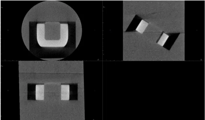
The standard Quart phantom (Quart GmbH, Zorneding, Germany) (Figure 2) was constructed for routine quality assurance purposes with CBCT volumes. This phantom is a cylinder approximately 16 cm in diameter, 15 cm in height and consists of a test object (test tool) in the center of a polyvinyl chloride (PVC) acrylic cylinder. The test tool appears as the block of material with an open square in the center and is made of polymethylmethacrylate (PMMA), air and PVC. The cylinder and test tool simulate the attenuation characteristics of free air, soft tissue, and bone. There is a built-in positioning tool that consists of a bubble level that is important for positioning the phantom properly. The quality assurance phantom can be used to evaluate image quality for field sizes 4 x 4 cm to large FOVS.
Figure 2: Standard Quart phantom. The standard Quart phantom consists of a test tool in the center of the phantom that is parallel to the axial plane.
The standard Quart phantom was compared to three modified Quart phantoms as described below. Modification one (Mod1) of the Quart phantom consisted of the test tool centered and oriented 30o to the axial plane (Figure 3). This modification was used to measure image quality parameters where the elements for measuring image quality were located at the center and angled with respect to the image acquisition plane at varying FOVs and dose protocols.
Figure 3: Quart phantom Mod1. This figure shows the test tool in the center of the phantom and angled with respect to the axial plane.
Modification two of the Quart phantom (Mod2) consisted of the test tool displaced to the periphery of the acrylic slab and parallel to the axial plane (Figure 4). This modification was utilized to measure image quality parameters where the elements for measuring image quality are at the periphery instead of the center of the phantom at varying FOVs and dose protocols.
was used to measure image quality parameters where the elements for measuring image quality were located at the periphery instead of the center and angled with respect to the axial plane at varying FOVs and dose.
Figure 5: Quart phantom Mod3. This figure shows the central element at the periphery of the phantom and angled with respect to the axial plane.
Each modified Quart phantom was compared to the standard Quart phantom and to each other. All CBCT volumes were acquired on the Carestream (CS) 9300 CBCT unit using different FOVs. The two large FOVs used were 17 x 11 cm and 17 x 6 cm. The two medium FOVs were 10 x 10 cm and 10 x 5 cm. The one small FOV was 8 x 8 cm. The five FOVs were used because they were large enough to image the entire Quart phantom test tool. Two dose protocols were used per FOV. These included a standard acquisition mode and feather acquisition mode. The standard acquisition mode is called regular dose from the manufacturer. In this study, the regular dose mode is abbreviated standard dose, standard resolution (SDSR). The feather acquisition mode is a low dose protocol and abbreviated as low dose, low resolution (LDLR) in this study.
When compared to the standard acquisition mode, the LDLR mode acquired images at about 80% lower dose for this study although it can range depending up on the CBCT unit [38]. This was due to different exposure settings. Reduction in exposure settings (kVp and mAs) while maintaining contrast and controlling noise is facilitated by increasing voxel size. However, the increase in voxel size does reduce resolution. The imaging parameters are listed in Table 1. The phantoms were positioned using the same tripod (SLK PRO 700DX) and the alignment laser
beams of the CS 9300 CBCT unit to center the phantom (Figure 6). The tripod stand had a built in leveling device in the sagittal and coronal planes. The Quart phantoms had a built in leveling device in the axial plane (bubble level). The alignment laser beams of the CS 9300 CBCT unit were used to confirm the proper position of the Quart phantoms, with the air segment of the test tool centered within the FOV. A scout image was then acquired to confirm the orientation and position of the Quart phantom before image acquisition.
Figure 6: Quart phantom positioning. The Quart phantom will be centered in the FOV of the CS9300 CBCT unit using the positioning lights as a guide. The same tripod and platform were used for all phantoms.
Each phantom was imaged three times at each FOV and each dose protocol. The volume data were exported from the CS 9300 CBCT unit software as uncompressed digital imaging and
Alternative (more detailed explanation of CNR calculation) In order to calculate the CNR, a rectangular region of interest (ROI) was selected between the PMMA and PVC sections of the phantom (Figure 7). The CNR was determined as the difference in mean voxel valuaes of the PMMA and PVC materials divided by the standard deviation for the PMMA material.
Alternative (more detailed explanation of MTF calculation) First, a rectangular region of interest (ROI) was selected for postprocessing of the voxels with dimensions parallel and
perpendicular to the edge (Figure 8). The software computed a row-by-row averaging of voxel profiles parallel to the PVC-air interface to acquire the edge spread function (ESF). Using the ESF profile, the line spread function (LSF) was calculated [39]. A Fourier-transformation of the LSF was used to calculate the MTF. MTF50% and MTF10% were determined from the MTF curve, which allowed for characterizing the spatial resolution.
Figure 7: CNR region of interest selection
Figure 8: MTF region of interest selection
In order for the software to calculate the image quality parameters, an image slice where the open block segment of the test tool produced a range of gray levels was imported. The slice of the test tool was selected by the lowest slice (closest to the most inferior surface) that was fully visible within the software for standardization of slice selection. All possible regions of interest (ROIs) were automatically displayed and could be manually adjusted. The ROI was defined by manually clicking and drawing a square or rectangle over the test tool within the loaded slice selection. The test result for Nyquist Frequency, contrast, noise, contrast-to-noise
protocol. Two researchers performed the analysis and recorded the data on an excel spreadsheet.
The researchers were standardized for slice selection, ROI selection, and there were no significant differences in the researcher’s calculations. Each data point was cross-checked for each researcher and Adobe PDF file of the test result to ensure accuracy and reliability of data recording.
Figure 9: Homogeneity ROI selection
Figure 10: Automatic software display of image quality parameters.
Mod1 and Mod3 volumes needed to be reoriented so that the test tool was in the axial plane before Quart DVTec image analysis. Dolphin Imaging Version 11.8.06.22 Premium was used to reorient the volumes without any loss of image quality. Figure 12 shows an example of modification one at the 8 x 8 cm FOV, SDSR prior to reorientation. Figure 13 shows
modification one at the 8 x 8 cm FOV, SDSR after reorientation.
Figure 12: Mod1 Quart phantom at the 8 x 8cm FOV, SDSR prior to reorientation
Figure 13: Mod1 phantom at the 8 x 8 cm FOV, SDSR after reorientation
Statistical analysis consisted of analysis of variance (ANOVA) for aim one, assessing the relationship between image quality parameters and image quality phantoms, in order to
determine if any significant differences existed between the MTF and CNR at the five different FOVs and two dose protocols both within and between the Quart phantoms. MTF and CNR were chosen to represent the image quality measures because they encompass spatial resolution, contrast, and noise for the calculations. ANOVA was considered for aim one because the data
RESULTS AIM ONE
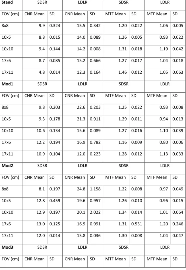
Objective measures of image quality were recorded and analyzed for each phantom, FOV, and dose protocol. The mean CNR, MTF, and standard deviations (SD) are summarized in Table 1.
Table 1: Dose protocols per FOV for all phantoms
SDSR LDLR
FOV (cm) Voxel Size (µm) kVp mAs Voxel Size (µm) kVp mAs
8x8 180 90 64 400 85 14.8
10x5 180 90 64 400 85 14.8
10x10 180 90 64 400 85 14.8
17x6 200 90 50.4 400 85 14.8
17x11 250 85 64.9 400 85 12
Table 2: Data summary. SDSR and LDLR refer to the dose protocols.
Stand SDSR LDLR SDSR LDLR
FOV (cm) CNR Mean SD CNR Mean SD MTF Mean SD MTF Mean SD
8x8 9.9 0.324 15.5 0.342 1.20 0.022 1.06 0.005
10x5 8.8 0.015 14.0 0.089 1.26 0.005 0.93 0.022
10x10 9.4 0.144 14.2 0.008 1.31 0.018 1.19 0.042
17x6 8.7 0.085 15.2 0.666 1.27 0.017 1.04 0.018
17x11 4.8 0.014 12.3 0.164 1.46 0.012 1.05 0.063
Mod1 SDSR LDLR SDSR LDLR
FOV (cm) CNR Mean SD CNR Mean SD MTF Mean SD MTF Mean SD
8x8 9.8 0.203 22.6 0.203 1.25 0.022 0.93 0.008
10x5 9.3 0.178 21.3 0.911 1.29 0.011 0.94 0.013
10x10 10.6 0.134 15.6 0.089 1.27 0.016 1.10 0.039
17x6 12.2 0.194 16.9 0.782 1.16 0.009 0.80 0.006
17x11 10.9 0.104 12.0 0.223 1.28 0.012 1.13 0.033
Mod2 SDSR LDLR SDSR LDLR
FOV (cm) CNR Mean SD CNR Mean SD MTF Mean SD MTF Mean SD
8x8 8.1 0.197 24.8 1.158 1.22 0.008 0.97 0.049
8x8 19.9 0.084 30.9 0.333 1.27 0.010 0.91 0.004
10x5 20.4 0.582 26.6 0.111 1.36 0.002 0.90 0.010
10x10 21.7 0.153 35.8 0.296 1.53 0.020 0.87 0.003
17x6 18.8 0.831 26.3 1.444 1.44 0.017 1.08 0.032
17x11 19.7 0.653 30.5 2.947 1.45 0.018 0.99 0.014
CNR
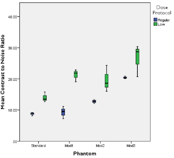
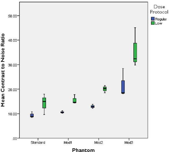
A three-way ANOVA was conducted to determine the effects of dose protocol, phantom, and FOV on CNR. There was a statistically significant three-way interaction between dose protocol, phantom, and FOV, p < 0.001. Because of the three-way interaction, a two-way ANOVA was performed to assess the effect of phantom (the primary explanatory variable) and dose protocol separately for each FOV. Statistical significance was set at an alpha level of 0.05 level. There was not a statistically significant simple two-way interaction between phantom and dose for the 10 x 5 cm FOV, (p = .1637), or for the 10 x 10 cm FOV, (p = .0978), or for the 17 x 6 cm FOV( p = .6975). There was a statistically significant simple two-way interaction between phantom and dose for the 8 x 8cm FOV (p = .0145), and for the 17 x 11 cm FOV (p < .001).
Therefore, an analysis of all possible pairwise comparisons was performed using a Bonferroni correction adjustment for statistical significance. The mean CNR values for each phantom and dose protocol are illustrated for each FOV in Figures 14–18.
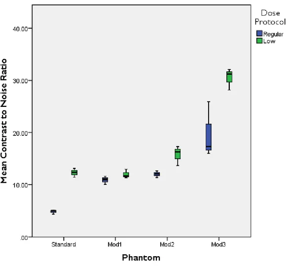
Figure 14: CNR of each phantom and dose protocol at the 8 x 8 cm FOV
Figure 15: CNR of each phantom and dose protocol at the 10 x 5 cm FOV
Figure 16: CNR of each phantom and dose protocol at the 10 x 10 cm FOV
Figure 17: CNR of each phantom and dose protocol at the 17 x 6 cm FOV
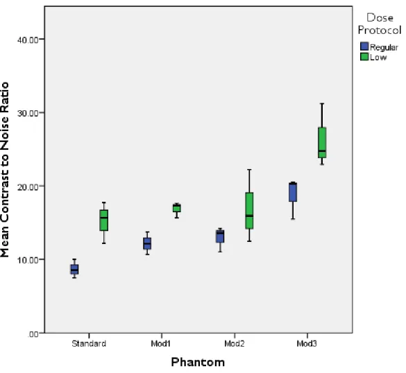
Figure 18: CNR of each phantom and dose protocol at the 17 x 11 cm FOV
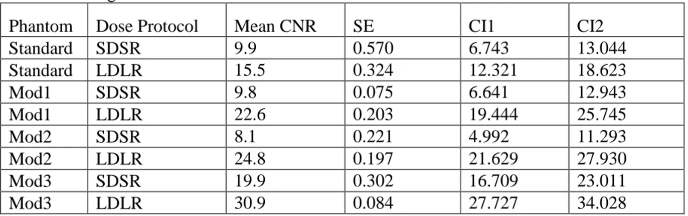
Table 3: Mean CNR, standard error (SE) and 95% confidence intervals (CIs) for each phantom and dose setting at the 8 x 8 cm FOV
Phantom Dose Protocol Mean CNR SE CI1 CI2
Standard SDSR 9.9 0.570 6.743 13.044
Standard LDLR 15.5 0.324 12.321 18.623
Mod1 SDSR 9.8 0.075 6.641 12.943
Mod1 LDLR 22.6 0.203 19.444 25.745
Mod2 SDSR 8.1 0.221 4.992 11.293
Mod2 LDLR 24.8 0.197 21.629 27.930
Mod3 SDSR 19.9 0.302 16.709 23.011
Mod3 LDLR 30.9 0.084 27.727 34.028
At the 8 x 8 cm FOV, modification three at SDSR had a statistically significantly higher mean CNR value than the standard phantom at SDSR, and modification one at SDSR. The mean CNR, standard error (SE), and 95% confidence intervals (CI1 and CI2) for each phantom and dose setting at the 8 x 8 cm FOV are listed in Table 3.
At the 8 x 8 cm FOV, modification two at LDLR had a statistically significantly higher mean CNR value than the standard phantom at both SDSR and LDLR, modification one at SDSR and modification two at SDSR. At the 8 x 8 cm FOV, modification one at LDLR had a statistically significantly higher mean CNR value than modification one at SDSR and
modification two at SDSR. The difference in means, confidence intervals, and the difference in the means are listed in Table 4.
Table 4: p values, difference in means, and 95% CIs for statistically significant interactions between phantoms and dose at the 8 x 8 cm FOV
Phantom Dose Protocol
Phantom Dose
Protocol p value
Difference in
means 95% CI1 95% CI2
Std-Reg M1-Low <0.001 -12.70 -19.978 -5.424 Std-Reg M2-Low <0.001 -14.89 -22.163 -7.609
Std-Reg M3-Reg 0.004 -9.97 -17.243 -2.689
Std-Reg M3-Low <0.001 -20.98 -28.261 -13.707
Std-Low M2-Reg 0.0477 7.33 0.052 14.606
Std-Low M2-Low 0.0078 -9.31 -16.584 -2.030
Std-Low M3-Low <0.001 -15.41 -22.683 -8.129
M1-Reg M1-Low 0.003 -12.80 -20.079 -5.525
M1-Reg M2-Low <0.001 -14.99 -22.264 -7.710
M1-Reg M3-Reg 0.0038 -10.07 -17.345 -2.791
M1-Reg M3-Low <0.001 -21.09 -28.362 -13.809
M1-Low M2-Reg <0.001 14.45 7.175 21.729
M1-Low M3-Low 0.0201 -8.28 -15.560 -1.006
M2-Reg M2-Low <0.001 -16.64 -23.914 -9.360
M2-Reg M3-Reg <0.001 -11.72 -18.994 -4.440
M2-Reg M3-Low <0.001 -22.74 -30.012 -15.458
M3-Reg M3-Low 0.0016 -11.02 -18.295 -3.741
At the 17 x 11 cm FOV, modification three at SDSR and LDLR had a statistically significantly different mean CNR value than all other phantoms at SDSR and LDLR.
Additionally, at the 17 x 11 cm FOV, modification three at SDSR had a statistically significantly different mean CNR value than modification three at LDLR. Mean CNR values for each
phantom at each dose for the 17 x 11 cm FOV are listed in Table 5. The difference in means, confidence intervals, and the difference in the means are listed in Table 6.
Table 5: Mean CNR, SE and 95% CIs for each phantom and dose setting at the 17 x 11 cm FOV Phantom Dose Protocol Mean CNR SE 95% CI1 95% CI2
Standard SDSR 4.8 0.666 2.108 7.557
Standard LDLR 12.3 0.014 9.589 15.038
Mod1 SDSR 10.9 0.782 8.175 13.624
Mod1 LDLR 12.0 0.104 9.279 14.728
Mod2 SDSR 12.0 0.991 9.312 14.761
Mod2 LDLR 15.8 0.531 13.034 18.483
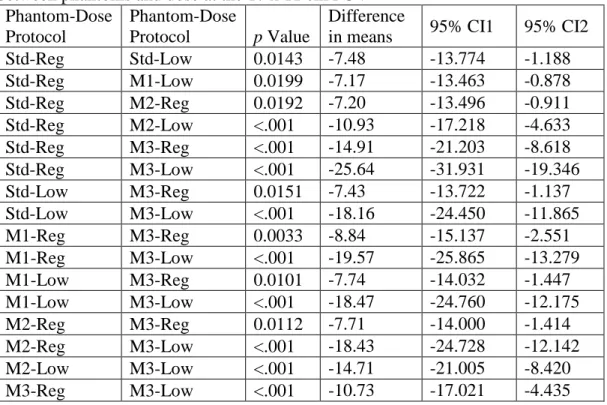
Table 6: p values, difference in means, and 95% CIs for statistically significant interactions between phantoms and dose at the 17 x 11 cm FOV
Phantom-Dose Protocol
Phantom-Dose
Protocol p Value
Difference
in means 95% CI1 95% CI2
Std-Reg Std-Low 0.0143 -7.48 -13.774 -1.188
Std-Reg M1-Low 0.0199 -7.17 -13.463 -0.878
Std-Reg M2-Reg 0.0192 -7.20 -13.496 -0.911
Std-Reg M2-Low <.001 -10.93 -17.218 -4.633 Std-Reg M3-Reg <.001 -14.91 -21.203 -8.618 Std-Reg M3-Low <.001 -25.64 -31.931 -19.346
Std-Low M3-Reg 0.0151 -7.43 -13.722 -1.137
Std-Low M3-Low <.001 -18.16 -24.450 -11.865
M1-Reg M3-Reg 0.0033 -8.84 -15.137 -2.551
M1-Reg M3-Low <.001 -19.57 -25.865 -13.279
M1-Low M3-Reg 0.0101 -7.74 -14.032 -1.447
M1-Low M3-Low <.001 -18.47 -24.760 -12.175
M2-Reg M3-Reg 0.0112 -7.71 -14.000 -1.414
M2-Reg M3-Low <.001 -18.43 -24.728 -12.142
M2-Low M3-Low <.001 -14.71 -21.005 -8.420
M3-Reg M3-Low <.001 -10.73 -17.021 -4.435
All simple pairwise comparisons were run for phantom modifications regardless of phantom type and regardless of dose for the 10 x 5 cm, 10 x 10 cm and 17 x 6 cm FOVs with a Bonferroni adjustment applied. Mean CNR values for these three FOVs adjusted for phantom type are listed in Table 7. There was a statistically significant difference in CNR values between SDSR and LDLR regardless of phantom type for the 10 x 5cm FOV, (p < 0.001), 10 x 10 cm FOV (p = 0.0037), and 17 x 6 cm FOV (p < 0.001), with the mean CNR for LDLR was statistically significantly higher than the mean CNR for the SDSR for each FOV.
Table 7: Mean CNR values for the 10 x 5, 10 x 10, and 17 x 6 cm FOVS at SDSR and LDLR regardless of phantom type
FOV (cm) Dose Protocol Mean CNR
10x5 Regular 12.8
10x5 Low 20.4
10x10 SDSR 13.6
10x10 Low 21.4
17x6 SDSR 13.1
17x6 Low 18.8
Mean CNR values for these three FOVS adjusted for dose are listed in Table 8. There was a statically significant difference in mean CNR values between the phantoms regardless of dose for the 10 x 5 cm FOV (p < 0.001), 10x10 cm FOV (p = 0.0089), and the 17 x 6 cm FOV (p
< 0.001) with the mean CNR for Mod3 being higher than the other phantom modifcations. The p values, difference in means, and 95% confidence intervals for statistically significant interactions between phantoms regardless of dose at the 10 x 5 cm, 10 x 10 cm and 17 x 6 cm FOVs are listed in Table 9.
Table 8: Mean CNR values for the phantoms at three FOVs without dose taken into account, SE, and CIs
Phantom FOV (cm) CNR Mean SE 95% CI1 95% CI2
Standard 10x5 11.4 0.052 8.984 13.831
Mod1 10x5 15.3 0.545 12.850 17.697
Mod2 10x5 16.2 1.415 13.787 18.634
Mod3 10x5 23.5 0.347 21.073 25.920
Standard 10x10 11.8 0.076 3.438 20.114
Table 9: p values, difference in means, and 95% CIs for statistically significant interactions between phantoms regardless of dose at three FOVs
Phantom Phantom
FOV
(cm) p value
Difference in
means 95% CI1 95% CI2
Std M2 10x5 0.039 -4.80 -9.408 -0.199
Std M3 10x5 <.001 -12.09 -16.694 -7.485
M1 M3 10x5 <.001 -8.22 -12.828 -3.619
M2 M3 10x5 0.0014 -7.29 -11.891 -2.682
Std M3 10x10 0.0334 -16.95 -32.792 -1.110
Std M3 17x6 <.001 -10.59 -15.087 -6.086
M1 M3 17x6 <.001 -7.99 -12.493 -3.492
M2 M3 17x6 <.001 -7.60 -12.103 -3.101
At the 10 x 5 cm FOV, modification three had a statistically significantly higher mean CNR than all other phantoms, regardless of dose. Additionally, at the 10 x 5cm FOV,
modification two had a statistically significantly higher mean CNR than the standard phantom, regardless of dose. At the 10 x 10 cm FOV, modification three had a statistically significantly higher mean CNR than the standard phantom, regardless of dose. At the 17 x 6 cm FOV, modification three had a statistically significantly higher mean CNR than all other phantoms, regardless of dose.
In summary, CNR significantly differed by phantom and dose protocol for the 8x8 and 17x11 cm FOV. CNR was higher on average for the LDLR and Mod3.
MTF
Table 10: Mean MTF 10% values and standard deviations (SD) for each dose protocol (SDSR and LDLR), phantom modifications and field of view.
Stand SDSR LDLR
FOV (cm) MTF Mean SD MTF Mean SD
8x8 1.20 0.022 1.06 0.005
10x5 1.26 0.005 0.93 0.022
10x10 1.31 0.018 1.19 0.042
17x6 1.27 0.017 1.04 0.018
17x11 1.46 0.012 1.05 0.063
Mod1 SDSR LDLR
FOV (cm) MTF Mean SD MTF Mean SD
8x8 1.25 0.022 0.93 0.008
10x5 1.29 0.011 0.94 0.013
10x10 1.27 0.016 1.10 0.039
17x6 1.16 0.009 0.80 0.006
17x11 1.28 0.012 1.13 0.033
Mod2 SDSR LDLR
FOV (cm) MTF Mean SD MTF Mean SD
8x8 1.22 0.008 0.97 0.049
10x5 1.26 0.010 0.96 0.015
10x10 1.34 0.014 1.01 0.064
17x6 1.31 0.531 1.20 0.246
17x11 1.30 0.008 1.04 0.047
Mod3 SDSR LDLR
FOV (cm) MTF Mean SD MTF Mean SD
8x8 1.27 0.010 0.91 0.004
A three-way ANOVA was conducted to determine the effects of dose, phantom and FOV on modulation transfer function 10%. There was a statistically significant three-way interaction between dose protocol, phantom and FOV (p < 0.001). Because of the three way interaction, a two-way ANOVA was performed to assess the effect of phantom (the primary explanatory variable) and dose protocol separately for each FOV. Statistical significance was set at the p <
0.05 level. Mean MTF values were higher at SDSR than at LDLR for all FOVs. The mean MTF values for each phantom and dose protocol are illustrated for each FOV in Figures 19–23.
Figure 19: MTF 10% of each phantom and dose protocol at the 8 x 8 cm FOV
Figure 20: MTF 10% of each phantom and dose protocol at the 10 x 5 cm FOV
Figure 21: MTF 10% of each phantom and dose protocol at the 10 x 10 cm FOV
Figure 22: MTF 10% of each phantom and dose protocol at the 17 x 6 cm FOV
Figure 23: MTF 10% of each phantom and dose protocol at the 17 x 11 cm FOV
There was not a statistically significant simple two-way interaction between phantom and dose for the 10x5cm FOV (p = 0.0921), or for the 10 x 10cm FOV (p = 0.1512). There was a statistically significant simple two-way interaction between phantom and dose for the 8 x 8cm FOV (p = 0.0003), for the 17 x 6cm FOV (p = 0.0116) and for the 17 x 11cm FOV (p < 0.0014).
Therefore, an analysis of all possible pairwise comparisons was performed using a Bonferroni adjustment for statistical significance.
Mean MTF values for each phantom at each dose for the 8x8cm FOV are listed in Table 11. At the 8 x 8cm FOV, modification three at SDSR had a statistically significantly lower mean MTF value than the standard phantom at SDSR (p < 0.001), the standard phantom at LDLR (p = 0.0017), modification one at SDSR (p < 0.001), modification two at SDSR (p < 0.001), and modification three at SDSR (p < 0.001).
Table 11: Mean MTF, SE and 95% CIs for each phantom and dose setting at the 8 x 8 cm FOV Phantom Dose Protocol MTF Mean SE 95% CI1 95% CI2
Standard SDSR 1.20 0.022 1.157 1.243
Standard Low 1.06 0.005 1.018 1.103
Mod1 SDSR 1.25 0.022 1.211 1.297
Mod1 Low 0.93 0.008 0.892 0.978
Mod2 SDSR 1.22 0.008 1.181 1.267
Mod2 Low 0.97 0.049 0.923 1.009
Mod3 SDSR 1.27 0.010 1.228 1.313
Mod3 Low 0.91 0.004 0.869 0.955
At the 8 x 8 cm FOV, modification three at LDLR had a statistically significantly higher mean MTF value than the standard phantom at LDLR (p < 0.001), modification one at SDSR (p
< 0.001), and modification two at LDLR (p < 0.001).
At the 8 x 8 cm FOV, modification two at SDSR had a statistically significantly higher mean MTF value than the standard phantom at LDLR and modification one at LDLR. At the 8 x 8 cm FOV, modification two at LDLR had a statistically significantly lower mean MTF value
Table 12: p values, difference in mean MTF value, and 95% CIs for interactions between phantoms and dose at the 8 x 8 cm FOV
Phantom-Dose Protocol
Phantom-Dose Protocol
p value Difference in mean MTF
95% CI1 95% CI2
Std-Reg Std-Low 0.0033 0.14 0.040 0.238
Std-Reg M1-Reg 0.5462 -0.05 -0.154 0.044
Std-Reg M1-Low <0.001 0.26 0.166 0.364
Std-Reg M2-Reg 0.987 -0.02 -0.123 0.075
Std-Reg M2-Low <0.001 0.23 0.135 0.333
Std-Reg M3-Reg 0.2719 -0.07 -0.170 0.028
Std-Reg M3-Low <0.001 0.29 0.189 0.387
Std-Low M1-Reg <0.001 -0.19 -0.293 -0.095
Std-Low M1-Low 0.0082 0.13 0.027 0.225
Std-Low M2-Reg 0.007 -0.16 -0.262 -0.064
Std-Low M2-Low 0.0661 0.09 -0.004 0.194
Std-Low M3-Reg <0.001 -0.21 -0.309 -0.111
Std-Low M3-Low 0.0017 0.15 0.050 0.248
M1-Reg M1-Low <0.001 0.32 0.220 0.418
M1-Reg M2-Reg 0.9563 0.03 -0.069 0.129
M1-Reg M2-Low <0.001 0.29 0.189 0.387
M1-Reg M3-Reg 0.9989 -0.02 -0.115 0.083
M1-Reg M3-Low <0.001 0.34 0.243 0.441
M1-Low M2-Reg <0.001 -0.29 -0.388 -0.190
M1-Low M2-Low 0.9503 -0.03 -0.130 0.068
M1-Low M3-Reg <0.001 -0.34 -0.435 -0.237
M1-Low M3-Low 0.9903 0.02 -0.076 0.122
M2-Reg M2-Low <0.001 0.26 0.159 0.357
M2-Reg M3-Reg 0.7281 -0.05 -0.146 0.052
M2-Reg M3-Low <0.001 0.31 0.213 0.411
M2-Low M3-Reg <0.001 -0.30 -0.404 -0.206
M2-Low M3-Low 0.5734 0.05 -0.045 0.153
M3-Reg M3-Low <0.001 0.36 0.260 0.458
At the 17 x 6 cm FOV, modification three at LDLR had a statistically significantly different mean MTF value than all other phantoms at SDSR and LDLR except for modifications 1 and 2 at LDLR. Mean MTF values for each phantom at each dose for the 17 x 6 cm FOV are listed in Table 13. The difference in means, confidence intervals and p values are listed in Table 14.
Table 13: Mean MTF, SE, and 95% CI for each phantom and dose setting at the 17 x 6 cm FOV Phantom Dose Protocol MTF Mean SE 95% CL1 95% CL2
Standard SDSR 1.27 0.017 1.193 1.355
Standard Low 1.04 0.018 0.957 1.120
Mod1 SDSR 1.16 0.009 1.083 1.246
Mod1 Low 0.80 0.006 0.717 0.879
Mod2 SDSR 1.31 0.014 1.224 1.387
Mod2 Low 1.20 0.036 1.116 1.279
Mod3 SDSR 1.44 0.017 1.357 1.519
Mod3 Low 1.08 0.032 0.996 1.158
Table 14: p values, difference in mean MTF, and 95% CIs for interactions between phantoms and dose at the 17 x 6 cm FOV
Phantom-Dose Protocol
Phantom-Dose Protocol
p value Difference in mean MTF
95% CI1 95% CI2
Std-Reg Std-Low 0.0091 0.24 0.048 0.423
Std-Reg M1-Reg 0.4956 0.11 -0.078 0.297
Std-Reg M1-Low <0.001 0.48 0.288 0.663
Std-Reg M2-Reg 0.9987 -0.03 -0.219 0.156
Std-Reg M2-Low 0.8379 0.08 -0.111 0.264
Std-Reg M3-Reg 0.112 -0.16 -0.351 0.024
Std-Reg M3-Low 0.0362 0.20 0.009 0.384
Std-Low M1-Reg 0.3389 -0.13 -0.313 0.062
Std-Low M1-Low 0.0077 0.24 0.053 0.428
Std-Low M2-Reg 0.0029 -0.27 -0.455 -0.080
Std-Low M2-Low 0.1296 -0.16 -0.347 0.029
Std-Low M3-Reg <0.001 -0.40 -0.587 -0.212
Std-Low M3-Low 0.9952 -0.04 -0.226 0.149
M1-Reg M1-Low <0.001 0.37 0.179 0.554
M1-Reg M2-Reg 0.2227 -0.14 -0.329 0.046
M1-Reg M2-Low 0.9982 -0.03 -0.221 0.154
At the 17 x 11 cm FOV, modification three at LDLR had a statistically significantly different mean MTF value than all other phantoms at SDSR. Mean MTF values for each phantom at each dose for the 17x11cm FOV are listed in Table 15. The difference in means, confidence intervals, and P values are listed in Table 16.
Table 15: Mean MTF, SE, and 95% CIs for each phantom and dose setting at the 17 x 11 cm FOV
Phantom Dose Protocol MTF Mean SE 95% CI1 95% CI2
Standard SDSR 1.46 0.012 1.390 1.537
Standard Low 1.05 0.063 0.979 1.126
Mod1 SDSR 1.28 0.012 1.208 1.355
Mod1 Low 1.13 0.033 1.058 1.205
Mod2 SDSR 1.30 0.008 1.227 1.374
Mod2 Low 1.04 0.047 0.962 1.109
Mod3 SDSR 1.45 0.018 1.381 1.528
Mod3 Low 0.99 0.014 0.919 1.066
Table 16: p values, difference in mean MTF, and 95% CIs for interactions between phantoms and dose at the 17 x 11 cm FOV
Phantom-Dose Protocol
Phantom-Dose Protocol
p value Difference in mean MTF
95% CI1 95% CI2
Std-Reg Std-Low <0.001 0.41 0.241 0.580
Std-Reg M1-Reg 0.0313 0.18 0.012 0.351
Std-Reg M1-Low <0.001 0.33 0.162 0.501
Std-Reg M2-Reg 0.0641 0.16 -0.007 0.333
Std-Reg M2-Low <0.001 0.43 0.258 0.598
Std-Reg M3-Reg 1 0.01 -0.161 0.179
Std-Reg M3-Low <0.001 0.47 0.301 0.640
Std-Low M1-Reg 0.0049 -0.23 -0.398 -0.059
Std-Low M1-Low 0.7387 -0.08 -0.249 0.091
Std-Low M2-Reg 0.0023 -0.25 -0.417 -0.078
Std-Low M2-Low 0.9999 0.02 0.152 0.187
Std-Low M3-Reg <0.001 -0.40 -0.571 -0.232
Std-Low M3-Low 0.9136 0.06 -0.110 0.230
M1-Reg M1-Low 0.1048 0.15 -0.020 0.319
M1-Reg M2-Reg 0.9999 -0.02 -0.188 0.151
M1-Reg M2-Low 0.0024 0.25 0.077 0.416
M1-Reg M3-Reg 0.0444 -0.17 -0.342 -0.003
M1-Reg M3-Low 0.0005 0.29 0.119 0.458
M1-Low M2-Reg 0.0524 -0.17 -0.338 0.001
M1-Low M2-Low 0.528 0.10 -0.073 0.266
M1-Low M3-Reg <0.001 -0.32 -0.492 -0.153
M1-Low M3-Low 0.1544 0.14 -0.031 0.308
M2-Reg M2-Low 0.0012 0.27 0.095 0.435
M2-Reg M3-Reg 0.0896 -0.15 -0.324 0.016
M2-Reg M3-Low 0.0002 0.31 0.138 0.477
M2-Low M3-Reg <0.001 -0.42 -0.589 -0.249
M2-Low M3-Low 0.9857 0.04 -0.127 0.212
M3-Reg M3-Low <0.001 0.46 0.292 0.631
All simple pairwise comparisons were ran for phantom modifications regardless of phantom type and regardless of dose for the 10 x 5 cm and 10 x 10 cm with a Tukey adjustment applied. Mean MTF values for these two FOVS adjusted for phantom type are listed in Table 17.
There was a statistically significant difference in MTF values regardless of phantom type for the 10 x 5 cm FOV (p < 0.001) and the 10x10cm FOV (p = 0.0002) with the mean MTF for SDSR statistically significantly higher than the mean MTF for the LDLR for each FOV. There was not a statically significant difference in mean MTF values regardless of dose for the 10x5cm FOV (p
= 0.7898) or the 10x10 cm FOV (p = 0.98).
Table 17: Mean MTF values for the 10 x 5 and 10 x 10 cm FOVs at SDSR and LDLR regardless of phantom type
FOV (cm) Dose Protocol Mean MTF
10x5 SDSR 1.30
DISCUSSION AIM ONE CNR
Voxel size, kVp, and mAs impacted the CNR (Table 3). The kVp, mA, and time were all higher for the standard dose protocol when compared to LDLR. Additionally, the voxel size for the LDLR was larger than the standard dose protocol at all FOVs. There was a statistically significant interaction between phantom and dose protocol at the 8 x 8 cm and 17 x 11 cm FOV.
The mean CNR values for LDLR were higher than SDSR for each phantom. All mean CNR values for LDLR were higher than all CNR values for SDSR regardless of phantom; an
exception was the mean CNR value at the 8 x 8 cm FOV for the modification three phantom at SDSR was higher than the mean CNR of the standard phantom at LDLR. However, this was not statistically significant. Usually, a SDSR would result in a higher CNR value than a LDLR due to the effect of more noise for the LDLR. However, this study found that the LDLR resulted in higher CNR. The results suggest that the larger voxel size of the LDLR counteracted the effect of reduced mAs producing an improved CNR. The opposite was found in another study by
Elkhateeb and co-workers where the CNR was lower with LDLR. This difference was accounted for by keeping the FOV and voxel size constant [40]. All SDSRs had a higher kVp than the LDLR by about 5 kVp. One would expect that there would be increased contrast with decreased kVp. However, the small increase of 5 kVp did not significantly affect the contrast.
The LDLR had lower kVp and lower mAs than the SDSR. The expected results were less signal (due to lower mAs and lower kVp) and more noise if the voxel size was the same.
However, voxelvolume was 4-11 times larger in LDLRs and thus had a larger signal and lower noise which counteracted the expected decrease in signal due to lower mAs and kVp. The most plausible explanation for the observation of a higher CNR on average for the LDLR when compared to the SDSR is that the difference in voxel size had more effect on the noise reduction than mAs had on signal.
The LDLR used a larger voxel size than the SDSR for all FOVs. Reduced kVp can increase contrast [41]. However, a lower kVp can also result in less signal as a result of a lower x-ray production efficiency, thus creating more noise. Elkhateeb and co-workers found that by keeping all exposure parameters the same, except kVp, that the LDLR had lower CNR [40]. Our study had multiple exposure parameters change which accounts for the different results. The large voxel size resulted in an increase in signal and counteracted the effect of a decrease in signal due to reduced mAs. CBCT uses isotropic voxels (cuboidal voxel). The matrix and pixel size of the detector determine voxel size in CBCT. If CBCT units have smaller voxels, the dose is usually increased to achieve a reasonable signal-to-noise ratio. The voxel size for the standard dose was smaller than the voxel size of the LDLR at all FOVs. Standard dose voxel sizes ranged
However, there was no statistically significant difference in CNR between modification one phantom and the standard or modification two phantoms regardless of dose at the 10 x 5, 10 x 10 or 17 x 6 cm FOVs.
Due to CBCT image acquisition techniques, there is a potential source of artifact at the periphery of the volume. This is called cone beam artifact and is caused by the divergence of the x-ray beam as it rotates around the patient in an axial plane [33]. Structures at the top and bottom of the image field are exposed only when the x-ray source is on the opposite side of the patient.
As a result, there is a potential for more noise and reduced contrast at the periphery of a CBCT volume. One would expect contrast to be the lowest and noise to be the highest. However, the CNR for Mod3 was found to be significantly larger than for any of the other phantoms. The reason for this finding is not well understood and speculative at this time. Possibly, the test tool was not far enough from the periphery or not rotated far enough out of the horizontal plane to see the cone beam effect. This would explain why CNR would not be decreased, but does not
explain why it actually increased. Alternatively, CNR may have been higher because of image processing algorithms designed by the manufacturer. Communication with the Quart phantom manufactured indicated that edge enhancement may have been applied in peripheral aspects of the phantom. While this does not fully explain the findings of this study, it at least suggests that the software may have played a role.
The quality and quantity of the x-ray beam depend on tube voltage (kVp) , tube current (mA) and exposure time (s). These settings can be adjusted, however, fixed exposure settings (manufacturer recommendations) were used for each FOV and dose setting. As mAs increases, exposure increases proportionally. The mAs for standard dose was approximately four times higher than that of LDLR. Higher mAs resulted in more signal. One would expect for the LDLR
to have a slightly higher contrast due to lower kVp but much higher noise than the SDSR, resulting in a lower CNR (an increase in the numerator or a decrease in the denominator will result in an increase in the CNR ratio). When both the numerator and denominator are increased or reduced, whether the CNR ratio increases or decreases is determined by the respective
changes in the both the numerator and denominator. This was not found to be true for the phantoms due to a larger voxel size for LDLR. Based upon the results, the difference in contrast was much less than the difference in noise due to the effect of larger voxel size in noise
reduction.
Subject contrast is the result of differential attenuation based on characteristics of the object. Influencing factors of subject contrast include the subject’s thickness, density, and atomic number. The atomic number and mass density were the same for each phantom. The thickness of the acrylic for modification one and modification three was greater than for the standard
phantom and for modification two. The reason for this was the need to accommodate the angled test tool. The greater the thickness of the subject, the more scatter is produced, which could lower contrast. Because of this, the modification 1 and modification 3 phantoms should have had lower contrast than the standard and modification 2 phantoms. At SDSR, there was no statistical difference between the modification 1 phantom and the standard or the modification two
MTF
Mean MTF values for the SDSR were higher than the mean MTF values for the LDLR for each field of view and for each phantom (Table 10). There was a statistically significant difference between the MTF values based upon dose protocols at the 8 x 8 cm, 17 x 6 cm, and 17 x 11 cm FOVs. There were no significant differences of the MTF values between the phantoms.
Other studies have shown similar results in that the smaller the voxel size, the higher that spatial resolution [42, 43]. The combined effect of higher kVp, higher mAs, and smaller voxel size of the SDSR had a positive effect on MTF, when compared to LDLR. In contrast, a study by Elkhateeb et al shows that there was no difference between MTF and changing voxel size (180 um, 300 um, and 500 um) or FOV (5 x 10 cm or 17 x 13.5 cm) using the same CBCT unit (CS 9300) [13, 40]. Similar results of no effect on MTF with changing voxels sizes were found in other studies [44, 45].
Reducing the field of view to the region of interest (collimation) is known to improve image quality by reducing scattered radiation [46]. Therefore, the smaller FOVs should theoretically have had a higher MTF than the larger FOVs. However, this was not found consistently throughout the five fields of view used in this study. The results were consistent with other studies that failed to identify any effect of FOV on MTF [7, 13]. This may be due to similar attenuation characteristics throughout the image quality phantoms. Other studies have shown that scatter can have an effect on spatial resolution, especially for low contrast structures [34, 47].
Generally, the higher the kVp, the more the scatter due to the energy of the scatter angle increasing and the scatter oriented in a more forward direction (towards the receptor). Additional scatter results in less contrast. Noise degrades edges and makes structure differentiation difficult,
especially between low contrast structures. This affects spatial resolution. Spatial resolution is the ability to distinguish between two adjacent structures as they become smaller and closer together [48]. The higher the spatial resolution is, the finer the detail in an image. Unaided human vision can distinguish approximately 10 lines per mm. Factors affecting spatial resolution include noise, motion blur, focal spot size, source-to-object distance, object-to-image distance and number of basis images [49]. The exposure settings also affected the image noise in other studies with larger amounts of exposure (higher kVp and/or higher mAs) associated with lower noise in CS9300 CBCT units [13, 44].
Spatial resolution in a CBCT image is also determined by the voxel size. CBCT uses isotropic voxels (voxels that are equal size in all three dimensions). Matrix and pixel size of the detector are the main determinant of voxel size. If the number of photons remains the same, a larger voxel size allows more photons to be detected and results in less image noise [50].
However, larger voxel sizes lower the spatial resolution. Smaller voxel sizes (higher resolution) usually require higher doses to maintain a reasonable signal-to-noise ratio. However, depending upon the diagnostic task, sometimes this is necessary. For example, a higher spatial resolution was found to result in higher detection of internal resorption than low resolution CBCT images [51].
decreased reconstruction time. The shortened scan time has been shown to reduce motion artifact, which is frequently encountered in orthodontics [52].
METHODS AND MATERIALS AIM TWO Subjective Image Quality (Aim Two)
The relationship of specific indicators of objective image quality to subjective measures of image quality of CBCT at varying FOVs and dose was evaluated. Two expert observers viewed images of a RANDO phantom (Figure 24) that were acquired with the CS 9300 CBCT unit utilizing the same image quality parameters, the same five FOVs and the two dose protocols used in the objective image quality study described previously. The RANDO phantom contains materials that simulates human tissue attenuation characteristics. Therefore, the RANDO phantom is suitable to be imaged for subjective image quality assessment.
Figure 24: RANDO phantom
Positioning of the RANDO phantom was accomplished by using the CS 9300 positioning
phantom. This helped to ensure the same orientation throughout the different FOVs and dose protocols.
The CBCT volumes were exported from the CS software as uncompressed DICOM files.
The volumes were imported into InVivoDental 5.0 (Anatomage Inc.) for landmark selection. The brightness and contrast settings were standardized for all FOVs, dose protocols, and landmarks in the center of the range in the software. The RANDO phantom was not repositioned or reoriented for any of the image reconstructions to maintain standardization. A Lenovo W540 laptop was used to make static images as JPG files of the selected images. The anatomic landmarks selected for the observer sessions were the hard palate in the coronal view (Figure 25), the hard palate in the sagittal view (Figure 26), the lateral pterygoid plates in the axial view (Figure 27), and the mental foramen in the coronal view (Figure 28).
Figure 25: Hard palate in the coronal view simulating the test tool location and orientation of the standard Quart phantom at the 17x11 cm FOV, SDSR.
Figure 26: Hard palate in the sagittal view simulating the test tool location and orientation of the Mod1 Quart phantom at the 17x11 cm FOV, SDSR.
Figure 28: Mental foramen in the coronal view simulating the test tool location and orientation of the Mod3 Quart phantom at the 17x11 cm FOV, SDSR.
The anatomical landmarks were selected for comparison based upon location, orientation, and visibility within the FOV. The anatomical landmarks were representative of central
structures, peripheral structures, and structures angled in relation to the axial acquisition plane [53]. The hard palate in the coronal view is located in the center of the volume and parallel to the axial plane, similar to the test tool of the standard Quart phantom. The hard palate in the sagittal view is located in the center of the volume and angled with respect to the image acquisition plane, similar to the test tool of Mod1. The lateral pterygoid plates in the axial view are located at the periphery of the volume and parallel to the image acquisition plane, similar to Mod2. The mental foramen in the coronal view is located at the periphery of the volume and at an angle to the image acquisition plane, similar to Mod3. The static images were imported into Qualtrics for comparison.