A dissertation submitted to the faculty at the University of North Carolina at Chapel Hill in partial fulfillment of the requirements for the degree of Doctor of Philosophy in the

STATISTICAL METHODS FOR GENETIC AND EPIGENETIC ASSOCIATION STUDIES

Kuan-Chieh Huang

A dissertation submitted to the faculty at the University of North Carolina at Chapel Hill in partial fulfillment of the requirements for the degree of Doctor of Philosophy in the

Department of Biostatistics in the Gillings School of Global Public Health.

Chapel Hill 2015

Approved by:

Mengjie Chen Ethan M Lange Yun Li

Kari E. North

Wei Sun

© 2015

Kuan-Chieh Huang

ALL RIGHTS RESERVED

ABSTRACT

Kuan-Chieh Huang: Statistical Methods for Genetic and Epigenetic Association Studies (Under the direction of Yun Li)

First, in genome-wide association studies, few methods have been developed for rare variants which are one of the natural places to explain some missing heritability left over from common variants. Therefore, we propose EM-LRT that incorporates imputation uncertainty for downstream association analysis, with improved power and/or computational efficiency. We consider two scenarios: I) when posterior probabilities of all possible genotypes are estimated;

and II) when only the one-dimensional summary statistic, imputed dosage, is available. Our methods show enhanced statistical power over existing methods and are computationally more efficient than the best existing method for association analysis of variants with low frequency or imputation quality.

Second, although genome-wide association studies have identified a large number of loci associated with complex traits, a substantial proportion of the heritability remains unexplained.

Thanks to advanced technology, we may now conduct large-scale epigenome-wide association

studies. DNA methylation is of particular interest because it is highly dynamic and has been

shown to be associated with many complex human traits, including immune dysfunctions,

cardiovascular diseases, multiple cancer, and aging. We propose FunMethyl, a penalized

functional regression framework to perform association testing between multiple DNA

simulations and real data clearly show that FunMethyl outperforms single-site analysis across a wide spectrum of realistic scenarios.

Finally, large studies may have a mixture of old and new arrays, or a mixture of old and new technologies, on the large number of samples they investigate. These different arrays or technologies usually measure different sets of methylation sites, making data analysis

challenging. We propose a method to predict site-specific DNA methylation level from one array to another – a penalized functional regression model that uses functional predictors to capture non-local correlation from non-neighboring sites and covariates to capture local correlation.

Application to real data shows promising results: the proposed model can predict methylation

level at sites on a new array reasonably well from those on an old array.

To my family and wife, I couldn’t have done this without you.

Thank you for all of your support along the way.

ACKNOWLEDGMENTS

I would like to offer countless thanks to my adviser, Yun Li, for her tireless support and

encouragement, and each of my committee members Wei Sun, Ethan Lange, Kari North, and

Mengjie Chen for their thoughtful contributions to this research. I would also like to thank my

collaborators from UNC-Chapel Hill for their invaluable comments and suggestions: Karen

Mohlke and Leslie Lange from the Department of Genetics for providing the real data used in the

illustrative real data example in chapter 3. Finally, I would like to thank my co-workers, friends,

and family for their patience and support of this work.

TABLE OF CONTENTS

LIST OF TABLES ...x

LIST OF FIGURES ... xi

LIST OF ABBREVIATIONS ... xii

CHAPTER 1: MOTIVATION AND BIOLOGICAL JUSTIFICATION ...1

CHAPTER 2: LITERATURE REVIEW ...6

2.1 Early Methods for Association Studies...6

2.1.1 GWAS ...7

2.1.2 EWAS ...8

2.2 Early Methods for DNA Methylation Prediction ...10

CHAPTER 3: EM-LRT ...12

3.1 Introduction ...12

3.2 Methods...13

3.2.1 A Hierarchical Modeling Framework to Simulate Data ...13

3.2.2 Expectation-Maximization Likelihood-Ratio Test ...14

3.2.3 Numerical Simulation ...17

3.3 Results ...18

3.3.1 MAF Threshold ...18

3.3.2 Empirical Type I Error Simulation ...19

3.3.3 Empirical Power Simulations ...20

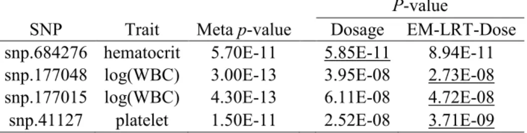
3.4 Real Data Application ...20

3.4.1 CLHNS ...20

3.4.2 WHI...22

3.5 Discussion ...23

CHAPTER 4: FUNMETHYL ...40

4.1 Introduction ...40

4.2 Methods...41

4.2.1 Estimation of DNA Methylation Function X

( ) t ...41

4.2.2 Estimation of DNA Methylation Effect β ( ) ^t ...43

4.2.3 Penalized Functional Linear Model ...44

4.2.4 Hypothesis Testing...44

4.3 Application to ARIC ...44

4.4 Real Data Simulation ...46

4.4.1 Empirical Type I Error ...46

4.4.2 Empirical Average Power ...47

4.5 Results ...48

4.5.1 Application to ARIC ...48

4.5.2 Q-Q Plot ...49

4.5.3 Empirical Type I Error ...49

4.5.4 Empirical Average Power ...50

4.6 Discussion ...51

CHAPTER 5: ACROSS-PLATFORM IMPUTATION OF DNA METHYLATION LEVELS USING PENALIZED FUNCTIONAL REGRESSION ...59

5.1 Introduction ...59

5.2 Methods...59

5.2.1 Estimation of X

( ) t ...60

5.2.2 Estimation of β ( ) t ...61

5.2.3 Selection of Local Covariate ...62

5.2.4 Grouping Probes ...62

5.2.5 Quality Filter ...62

5.2.6 Imputation Quality Assessment ...63

5.2.7 Simulation of Association Study ...63

5.3 Simulation Results ...64

5.4 Application to AML Data Set ...64

5.5 Discussion ...66

CHAPTER 6: CONCLUDING REMARKS ...77

REFERENCES ...79

LIST OF TABLES

Table 1 Rejection Sampling vs. Dosage Approximation for Estimation ... 28

Table 2 Type I Error Rate at Significance Level = 5E-02 ... 29

Table 3 Type I Error Rate at Significance Level = 5E-05 ... 30

Table 4 Associated Variants with R

≤ 0.3 in the CLHNS Study ... 31

Table 5 Associated Variants with MAF < 5% in the WHI Study ... 32

Table 6 One-sample T-test for Type I Error ... 33

Table 7 Empirical Type I Error (Gene BCL6) ... 54

Table 8 Quantiles of Imputation MSE and R

... 69

LIST OF FIGURES

Figure 1 MAF Threshold: Rejection Sampling (Black) vs. Dosage Approximation (Grey) ... 34

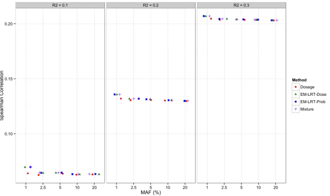
Figure 2 Spearman Correlation with Gold Standard P-values... 35

Figure 3 Power Comparison ... 36

Figure 4 Q-Q Plot for Null Variants with Low Imputation Quality in the CLHNS Study ... 37

Figure 5 Computing Time: Mixture Method vs. EM-LRT-Prob ... 38

Figure 6 Estimated vs. True Imputation (Rsq vs. R

) ... 39

Figure 7 Q-Q Plot of P-values Generated by Region-based Tests and Single-probe Test ... 55

Figure 8 Empirical Power with Small DNA Methylation Effect (d = 0.5) ... 56

Figure 9 Empirical Power with Moderate DNA Methylation Effect (d = 1) ... 57

Figure 10 Empirical Power with Large DNA Methylation Effect (d = 1.5) ... 58

Figure 11 Empirical Cumulative Distribution of Imputation MSE for Probes Showing Large Variation in AML Data Set ... 70

Figure 12 Empirical Cumulative Distribution of Imputation R

for Probes Showing Large Variation in AML Data Set ... 71

Figure 13 Empirical Power of Simulated Association Tests Across A Spectrum of Effect Size c... 72

Figure 14 The DNA Methylation Profile of the Target Probe vs. 10 Selected Local Probes ... 73

Figure 15 The Individual-specific Density Plot of DNA Methylation Level ... 74

Figure 16 Scatter Plot of Imputation MSE vs. Under-Dispersion Measure ... 75

Figure 17 Scatter Plot of Imputation R

vs. Under-dispersion Measure ... 76

LIST OF ABBREVIATIONS

AML Acute Myeloid Leukemia

ARIC Atherosclerosis Risk in Communities Study BMI Body Mass Index

bp Base Pair

CARDIA Coronary Artery Risk Development in Young Adults CLHNS Cebu Longitudinal Health and Nutrition Survey CNV Copy Number Variant

EWAS Epigenome-wide Association Study GCV Generalized Cross-Validation GWAS Genome-wide Association Study HM27 HumanMethylation27

HM450 HumanMethylation450 JHS Jackson Heart Study LD Linkage Disequilibrium LDL Low Density Lipoprotein MaCH Markov Chain Haplotyper MAF Minor Allele Frequency OLS Ordinary Least Square

PC Principle Component

PLINK PuTTY Link

REML Restricted Maximum Likelihood

SKAT SNP-Set (Sequence) Kernal Association Test

SKAT-O Optimal SNP-Set (Sequence) Kernal Association Test SNP Single Nucleotide Polymorphism

TCGA The Cancer Genome Atlas

TFBS Transcription Factor Binding Site

WC Waist Circumference

WHI Women’s Health Initiative

CHAPTER 1: MOTIVATION AND BIOLOGICAL JUSTIFICATION In this document, we propose statistical methods for assessing association between a genetic variant or sets of epigenetic marks and complex human traits. Because large studies may have a mixture of old and new arrays, or a mixture of old and new technologies, on the large number of epigenetic marks investigated, we also propose a method to predict site-specific DNA methylation level from one array to another. This section provides an overview of the biological problems we are interested in and some of the statistical strategies employed in an attempt to solve them.

To begin, DNA is a double-stranded molecule consisting of four nucleic acid

components: Adenine (A), Cytosine (C), Guanine (G) and Thymine (T). DNA is found in the nucleus of the vast majority of plant and animal cells and has been compared to a blueprint for the organism in which it is found. Humans have 22 autosomes, in addition to the sex

chromosomes X and Y and mitochondrial DNA, accounting for over 5 billion base pairs in total.

We will consider primarily autosomal DNA, for which each individual possesses two copies, one

inherited maternally and the other paternally. Over 99% of the DNA sequence is the same across

humans (Morris and Zeggini 2010); however, there are a large number of ways in which human

DNA sequence can differ from one another in a single region including microsatellites, copy

number variations (CNVs), insertions, deletions, inversions and single nucleotide polymorphisms

(SNPs). Any one of these can be called a genetic variant, meaning that it contains a sequence of

nucleic acids that is different from the consensus sequence or from what is most common.

A SNP is one such genetic variant that occupies only one base pair. As previously stated, much of the genome is shared across humans; however, some of these variants, SNPs included, are quite common with variant or minor allele frequency (MAF) near 0.5. In the 1990’s

microarray technologies from companies like Affymetrix and Illumina began to capitalize on these common SNPs in the form of genome-wide SNP platforms. Today these technologies can accurately assess up as many as 1 million pre-selected SNPs [e.g. the Affy Axiom or Illumina 1M], however these technologies are limited in that they cannot discover new variants.

As SNP genotyping technology advances, it is now possible to genotype hundreds of thousands of alleles in parallel. This has made it possible to rapidly scan markers across the complete genomes of many people; therefore, the association between the traits of interest and millions of markers could be tested. Recently, genome-wide association studies (GWASs) have identified SNPs related to several complex diseases. The completion of The International HapMap Project has provided a possibility to impute missing genotypes that were not directly genotyped from a cohort or case-control study but were genotyped in the reference samples.

Genotype imputation relies on the fact that even two unrelated individuals can share short

stretches of haplotype inherited from distant common ancestors. Several methods have been

proposed to take imputation into account in genome-wide association studies (GWASs). These

existing methods, however, have focused primarily on common variants, which have been the

focus of the past wave of GWASs examining either only directly genotyped (or typed) markers,

or typed and untyped markers imputed with the aid of smaller scale, lower density reference

panels such as those from the International HapMap Project. However, few (if any) methods

have been developed for rare variants which have been receiving intensive attention in the past

half decade as one of the natural places to explain some missing heritability left over from

common variants, for almost all complex traits studied in the genetics community. In the third chapter, an expectation-maximization likelihood-ratio test (EM-LRT) is developed. This method can accommodate either posterior genotype probabilities (EM-LRT-Prob) or imputed dosages (EM-LRT-Dose). We evaluated our methods and compared them with existing methods through extensive simulations. Our methods clearly show enhanced statistical power over existing methods and computationally more efficient alternative to the best existing method for association analysis of variants with low MAF or imputation quality. We also applied our methods to two data sets: the Cebu Longitudinal Health and Nutrition Survey (CLHNS) and Women’s Initiative Study (WHI) of Blood Cell Traits. Consequently, all methods have proper control of type I error and our methods generated more significant p-values (and better

approached truth in all cases), suggesting power enhancement using our methods.

Although GWASs have identified a large number of loci associated with complex traits, a substantial proportion of the heritability remains unexplained. For example, the >200 loci

identified for height can only explain ~20% out of the ~80% total estimated heritability. Recent technological advances have allowed us to conduct large-scale epigenome-wide association studies (EWASs). DNA methylation is of particular interest because it is highly dynamic (Rakyan et al. 2011) and has been shown to be associated with many complex human traits, including immune dysfunctions, cardiovascular diseases, multiple cancer, and aging. Typically, methylation level at hundreds of thousands of sites is measured and each of these sites is examined separately (i.e., single-site analysis). However, because of the correlation structure among the sites and because many of them fall in naturally defined regions (e.g., belonging to the same gene; belonging to the same regulatory region such as an enhancer or DNAse

hypersensitivity site), it is conceptually straightforward to imagine achieving enhanced statistical

power by performing region-based test (that is, simultaneously testing multiple sites together) especially when there are multiple low or moderate signals in that region. In the fourth chapter, a penalized functional region-based model is proposed to perform the association testing between DNA methylation marks in a region (explanatory variable) and quantitative trait (response variable). We evaluated our methods and compared them with the benchmark single-site analysis through extensive real data simulations. All the methods have proper control of type I error;

however, our methods have enhanced statistical power over the single-site analysis across various settings. Moreover, our methods have much higher statistical power than the existing region-based tests SKAT and SKAT-O. This work is close to finish and we expect to submit the manuscript soon.

Lack of high-throughput profiling technologies used to hinder our understanding of the dynamic state of DNA methylation. Fortunately, geneticists are embraced nowadays by

technological advances. For the study of DNA methylation, for example, technological advances constantly provide us with more choices to measure DNA methylation patterns across the

genome, including multiple commercial arrays, multiple sequencing-based technologies or

protocols (Laird 2010). However, large studies may have a mixture of old and new arrays, or a

mixture of old and new technologies, on the large number of samples they investigate. These

different arrays or technologies usually measure different sets of methylation sites, making data

analysis challenging, if not even impossible. For example, Illumina HumanMethylation27

(HM27) and HumanMethylation450 (HM450) BeadChip are two common microarrays used by

the Cancer Genome Atlas (TCGA) project. In several TCGA studies, the DNA methylation

profiles of samples collected more recently were measured by HM450, while the others were still

measured by HM27. Then when researchers want to utilize data of all samples for downstream

analysis, they can only focus on probes shared between two platforms for simplicity, since re- evaluating all samples using HM450 is both costly and time-consuming. In the fifth chapter, a penalized function regression model is proposed for DNA methylation prediction. We applied the proposed model to a large-scale methylation data set from acute myeloid leukemia patients.

As a result, the proposed model can produce accurate imputations when the reference panel

(training set) and the target panel (testing set) characterize the same tissue under similar

conditions.

CHAPTER 2: LITERATURE REVIEW

This section presents a partial review of many of the papers previously published on the topic of association studies. It is by no means complete since the number of these papers is quite large; however, it is an attempt to show the development of several methods used for these studies.

2.1 Early Methods for Association Studies

Genotype imputation has become standard practice in modern genetic studies (Browning and Browning 2008; Li et al. 2009; Li et al. 2010; Marchini and Howie 2010). For each untyped variant imputed, standard imputation methods estimate posterior probabilities of all possible genotypes. For example, when the untyped variant is bi-allelic with alleles A and B, we obtain posterior probabilities for A/A, A/B, and B/B with the constraint of summation being one. Such probability information can be further summarized into degenerate one-dimensional summary statistics including the mode (the best-guess genotype, or the genotype with the highest posterior probability), or the mean (the imputed dosage).

Since association analysis with phenotypes of interest rather than genotype imputation per se is usually of the ultimate interest, development and evaluation of post-imputation association strategies have therefore attracted considerable attention from the research

community (Chen and Abecasis 2007; Lin et al. 2008; Aulchenko et al. 2010; Pei et al. 2010;

Jiao et al. 2011; Kutalik et al. 2011; Zheng et al. 2011; Acar and Sun 2013; Liu et al. 2013b).

modeling complexity, computational efficiency and statistical power, have been shown analytically to be optimal among methods based on one-dimensional summary statistics (Liu et al. 2013b), and thus have been most commonly adopted in recent imputation-aided genome- wide association studies (Chambers et al. 2011; Auer et al. 2012; Dastani et al. 2012; Berndt et al. 2013). On the other hand, explicitly modeling the probabilities of all possible genotypes using the mixture of regression models (abbreviated Mixture hereafter and detailed below) has the best performance in terms of statistical efficiency, particularly with low imputation quality, but at the cost of increased computational complexity (Zheng et al. 2011).

GWASs have successfully identified sites associated with common diseases but still, a substantial proportion of the causality remains unexplained. In fact, GWASs only study the association between trait and genetic variants at the DNA level, and also some single nucleotide polymorphisms (SNPs) associated with common diseases are not localized near any gene in the pathways involved. Therefore, the unexplained causality could be found in epigenetic variation.

Based on the experiences from GWASs, it is inevitable to perform large-scale and systematic studies to detect the epigenetic variation. Epigenome-wide association studies (EWASs) allow us to identify genome-wide epigenetic variants associated with common diseases. DNA methylation is of particular interest because it is highly dynamic and, also the profiling technology for both array- and sequencing-based methods has been well developed. Among these technologies, the whole-genome bisulphite sequencing provides the highest coverage and resolution.

2.1.1 GWAS

We will introduce several existing methods that are widely used in GWAS. First, let

F

= ( f

, f

, f

) represent the genotype probability vector and X

represent a particular feature of

the imputation procedure

X

= argmax

j∈{0,1,2}

{ } f

f

+ 2 f



 



, ,

Best-guess Dosage

Best-guess and Dosage methods directly regress the trait Y

on a particular feature X

adjusting for the covariates Z

Y

= β

+ β

X

+ γ ^Z

+ ε

where ε

^{~ N 0,} ( ) σ

and i = 1, 2, …, N with N being the sample size. Next, the Mixture method (Zheng et al. 2011) fits the following mixture of regression model

Y

= f

⋅ g

( β

, β

, γ ^, ε

)

j=0

∑

where g

( β

, β

, γ ^, ε

) ^{= β}

^{+ j ⋅ β}

^{+ γ Z}

^{+ ε}

. To estimate the parameters ( β

, β

, γ ) in the Mixture model, the log-likelihood function is maximized using the Nelder-Mead Simplex Method (Nelder and Mead 1965), implemented in R package optim.

2.1.2 EWAS

Typically, DNA methylation level at hundreds of thousands of sites is measured and each of these sites is examined separately (i.e., single-site analysis). For a given CpG site j, the

methylated (M

) and unmethylated (U

) signal intensities are combined to methylation β-values:

β − value

= max M (

, 0 )

max M (

, 0 ) ^{+ max U} ( )

^{, 0 + α}

where the inclusion of an offset α

= 100 is recommended as a stabilization in the situation when

both methylated and unmethylated signal intensities are small. By definition, the β-values are

methylation. Most regression models used in EWAS treats DNA methylation level as response variable and disease-related phenotypes as explanatory variables. To directly use β-values without transformation, Beta regression (Ferrari and Cribari-Neto 2004) designed for modeling proportions bounded to [0,1] is often used.

It was later proposed to use the log

ratio of the methylated to unmethylated signal intensities (Allison et al. 2006):

M − value

= log

max M (

, 0 ) ^{+ α}

max U ( )

, 0 ^{+ α}





 





 

where α

= 1 is usually specified and the M-values are therefore defined on ( −∞ , ∞ ) . It has also been shown that after ignoring α

^and α

, there is a logit (with base 2) relationship between β- values and M-values:

M − value

≈ log

β − value

1 − β − value



  

 

As a result, after transforming β-values, the linear regression model for CpG site j is fit as

M

= α + γ ^Z

+ ε

, where M

is M-value

at site j, Z

is the covariate vector, ε

~ N 0, ( ) σ

^{, and i =}

1, 2, …, N with N being the sample size. Moreover, if one wants to adjust for batch effect, a

mixed model can be easily adopted by specifying a batch-specific random effect in the model. In

addition, the feature selection using test statistics is similar for M- and β-values for relatively

large sample sizes but M-values allow more reliable identification of true positives for small

sample sizes (Zhuang et al. 2012).

2.2 Early Methods for DNA Methylation Prediction

DNA methylation is an important epigenetic modification involved not only in normal development (Reik 2007; Smith and Meissner 2013) but also in risk and progression to many diseases (Bergman and Cedar 2013). It has been shown to play a key role in the regulation of gene transcription, X-inactivation, cellular differentiation, as well as other critical processes such as aging (Bird 2002; Gonzalo 2010). Recently, the emergence of powerful technologies such as microarray-based DNA methylation studies (Bibikova et al. 2011) and whole-genome bisulfite sequencing (Harris et al. 2010) has enabled the profiling of DNA methylation levels at high resolution. Numerous studies employed these high-throughput approaches to characterize changes of DNA methylation patterns and their corresponding tissue and disease-specific differentially methylated regions on a genome-wide scale (Irizarry et al. 2009; Berman et al.

2011; Varley et al. 2013).

As new technology emerge, researchers tend to replace old methylation profiling platforms with new ones. However, different platforms usually target CpG sites at different locations and resolutions, which hinder joint analysis of data from different platforms. For instance, Illumina HumanMethylation27 (HM27) and HumanMethylation450 (HM450) BeadChip are two common microarrays used by The Cancer Genome Atlas (TCGA) project.

While HM27 investigates 27,578 CpG sites predominantly located near CpG islands, HM450

provides broader coverage with 485,577 probes spanning 96% of CpG islands and 92% of CpG

shores across a larger number of genes. Several TCGA studies have used HM450 to gather

methylation profile data for more recently collected samples while still using HM27 to measure

DNA methylation in the older test subjects. These mixed profiles compel researchers to focus on

those probes shared between the two platforms when using the data for downstream analysis, as

re-evaluating all samples using HM450 is not only expensive but also time-consuming.

Most existing methods for DNA methylation prediction assume the DNA methylation is

binary, the DNA methylation status is 0 for unmethylated and 1 for methylated. They also have

limited predictions to specific regions of the genome. Moreover, most existing methods attempt

to predict the DNA methylation level or status using HM450 probes as well as some features,

such as DNA composition, predicted DNA structure, repeat elements, transcription factor

binding sites (TFBSs), evolutionary conservation, and etc.

CHAPTER 3: EM-LRT

3.1 Introduction

Limited evaluations of existing methods (including methods that explicitly model posterior probabilities) on variants with low imputation quality suggest much reduced power compared with accurately imputed variants, for instance, as demonstrated in Figure 2 and 3 of (Zheng et al. 2011) and Figure 2 of (Liu et al. 2013b) Analysis of variants with low imputation quality is not surprisingly a challenging problem due to the low correlation between imputed and true genotypes. It is nevertheless an increasingly important problem because as sequencing-based reference panels continue to grow (Altshuler et al. 2012; Fu et al. 2013)we have increasingly more well imputed markers but also even more markers with relatively low imputation quality, particularly at markers with lower allele frequencies (Duan et al. 2013a)(Altshuler et al. 2010b;

Liu et al. 2012; Zhang et al. 2013; Duan et al. 2013b). It is thus highly warranted to seek

alternative and potentially more efficient methods to model imputation uncertainty for these

markers. In this chapter, we develop expectation-maximization likelihood-ratio tests (EM-LRT)

that can accommodate either posterior genotype probabilities, when available (EM-LRT-Prob),

or imputed dosages (EM-LRT-Dose). Simulations and real data application demonstrate the

validity of the proposed methods and suggest them as a computationally more efficient

alternative to the best existing method (Mixture) for association analysis of variants with low

MAF or imputation quality.

3.2 Methods

3.2.1 A Hierarchical Modeling Framework to Simulate Data

We adopt a hierarchical model that generates posterior probabilities, imputed dosages, and true genotypes using marker-specific information including minor allele frequency (MAF) and imputation quality measure (R

), as well as a quantitative trait with which we test for genetic association. The model has three stages: the first stage generates genotype probabilities based on marker-specific information (genotype probability stage); the second stage employs a

multinomial distribution with probabilities from the first stage to generate allele counts (allele count stage); and the final stage fits a linear regression model to generate quantitative trait values

(trait stage).

Genotype Probability Stage. For a specific marker with MAF q and imputation quality R

, the genotype probability vector F

= ( f

, f

, f

) for the i-th sample is drawn from a Dirichlet distribution with parameters α = ( α

, α

, α

) ^{, where f}

is the probability of having j copies of the minor allele for the i-th sample and f

= 1

j=0

∑

. The parameters in the Dirichlet distribution are:

α

= ( ) 1− q

^{c , α}

^{= 2q 1} ( ) ^{− q c , α}

^{= q}

^{c with c = R}

( ^{1 − R}

) . Here we give some brief

explanations. First, this distribution gives reasonable expected values for F

= ( f

, f

, f

) ^such

that E f ( )

⁼ ( ) ^{1− q}

^{, E f} ( )

^{= 2q 1−} ( ) ^{q , and E f} ( )

^{= q}

, which are the expected probabilities of

having 0, 1, or 2 copies of minor alleles assuming Hardy-Weinberg Equilibrium. Next, when R

approaches to 1, F

= ( f

, f

, f

) approaches to a distribution that takes three possible values,

(1,0,0), (0,1,0), and (0,0,1) (i.e., the probability of having a particular genotype is either 0 or 1),

which is the expected situation when there is no imputation ambiguity. Given the genotype

probability vector, the imputed dosage is D

= f

+ 2 f

.

Allele Count Stage. The allele count vector X

= ( x

, x

, x

) for the i-th sample is drawn from a multinomial distribution with genotype probabilities specified in the previous stage, where x

= 1 if the i-th sample has j copies of the minor allele; and 0 otherwise, with the constraint of x

=1

j=0

∑

. Additionally, the genotype G

for the i-th sample is generated using this

allele count vector, specifically G

= x

+ 2x

. Our simulation framework, taking imputation

quality R

into account using c above, renders ^corr

( ^G

^{, D}

) = ^R

.

Trait Stage. In the final stage, a linear regression model is used to generate quantitative trait Y

using genotype G

and covariates Z

, Y

= β

+ β

G

+ γ ^Z

+ ε

, where ε

~ N 0, ( ) σ

^{and i =} 1, 2, …, N.

3.2.2 Expectation-Maximization Likelihood-Ratio Test

Our primary goal is to test for marker-trait association when marker genotypes G are not directly observed but rather imputed. We propose the following expectation-maximization likelihood ratio tests (EM-LRT). We consider two common scenarios after genotype imputation:

1) when posterior probabilities of genotypes are available and 2) when only dosages are available.

Scenario I: When Posterior Probabilities Are Available [EM-LRT-Prob]. Under this scenario, the true genotype G

is missing but genotype probability vector F

= ( f

, f

, f

) ^is

estimated, i = 1, 2, …, N with N being the sample size. Given the observations ( y

, G

, z

, f

)

where f

is the observed value for F

, the complete data likelihood is

L

( β ^, σ ^, γ ^{y, G, z, f} ) ⁼ ∏

^{f y} (

^G

^{, z}

^{, f}

) ^{⋅ P G} (

^z

^{, f}

) ⁼

^{f y} (

^G

^{, z}

) ^{⋅ P G} ( )

^f

^∝ ∏

^{f y} (

^G

^{, z}

)

∏

where the second equality holds because trait y

is independent of genotype probability vector f

conditional on true genotype G

and true genotype is independent of covariates z

conditional on genotype probability vector. Therefore, with Gaussian distribution, the corresponding complete- data log-likelihood is

l

( β , σ , γ y, G, z, f ) ^∝

^{− log σ −  y}

^{− ( β}

^{+ β}

^G

^{+ γ z}

^{) }

^{2 σ}

∑

In this complete data log-likelihood, terms involving true genotype G

, namely G

and G

, are not observed and will be replaced in the E-step by their conditional expectations given the observed data. Their conditional expectations are

E G (

y

, f

, z

) ⁼

^G

^{⋅ P G} (

^y

^{, f}

^{, z}

) ^{= C}

∑

⋅

G

⋅ P y (

G

, z

) ^{⋅ P G} ( )

^f

∑

E G (

y

, f

, z

) ⁼

^G

^{⋅ P G} (

^y

^{, f}

^{, z}

) ^{= C}

∑

⋅

G

⋅ P y (

G

, z

) ^{⋅ P G} ( )

^f

∑

where C =

f y (

G

, z

) ^{⋅ P G} ( )

^f

∑

^{, and P G} ( )

f

^{= f}

^f

^f

^.

In the M-step, the maximum likelihood estimates of the parameter θ = ( β

, β

, γ ^, σ ) ^are

obtained as follows:

ˆ ( β

, ˆ β

, ˆ γ ) ⁼ { ^{[ I, G, Z ]}

^{[ I, G, Z ]} }

^{[ I, G, Z ]}

^{Y = I}

T

I I

G I

Z G

I G

G G

Z

Z

I Z

G Z

Z





 

 





 

 

−1

I

Y G

Y Z

Y





 

 





 

 

ˆ σ

= ( Y − β ˆ

− G ˆ β

− Z ˆ γ )

( ^{Y − β ˆ}

^{− G ˆ β}

^{− Z ˆ γ} ) ⁿ

We repeat the E-step and M-step until convergence ( δ < 10

).

To speed up the EM algorithm, we suggest using the naïve parameter estimates as

starting values, that is, the parameter estimates derived by fitting a simple linear regression on

trait Y using dosage D and covariates Z (a.k.a Dosage or standard method). Our EM-LRT-Prob approach shares some similarity with the seminar work by Lander and Botstein (Lander and Botstein 1989) for interval mapping, in which the authors also used mixture model framework, treating genotypes at quantitative trait sites as missing data.

Scenario II: When Only Dosages Are Available [EM-LRT-Dose]. We propose a framework that first uses the conditional (on dosages) distribution to sample genotype probabilities given the imputed dosages, and then apply the EM algorithm detailed above in Scenario I.

First, we derive the probability density function for f

, the probability of having one copy of the minor allele conditioning on imputed dosage

f f (

= p D

) ⁼ _B ^C _{( ) α} ^{′ ⋅  1 − 0.5 D (}

^{+ p ) }

^p

^{ 0.5 D (}

^{− p ) }

where C’ is the normalizing constant, p ∈ ^ 0, min 2 ( − D

,1, D

) ^{ , and B} ( ) ^⋅ is the beta function [Appendix B]. Second, we select the envelope function g p ( ) ^{= max}

^{f f} (

^{= p D}

) such that

f p ( ) ^{≤ g p} ( ) for all p. Third, we perform the following steps to sample f

: 1) generate

p ~ U 0, min 2 ( ( − D

,1, D

) ) ; 2) generate U ~ U 0,1 ( ) ; 3) accept if U < f p ( ) ^{g p} ( ) . Finally, we calculate f

and f

using the relationship D

= f

+ 2 f

and f

= 1

j=0

∑

^.

The drawback of the above rejection sampling approach is that it can be computationally

rather expensive especially when the envelope function is large. Fortunately, we can use an

approximation approach when MAF is not high. For example, when MAF is low enough, the

probability of having two copies of the minor allele is close to zero. In that case, we adopt an

probability of having one copy of the minor allele to dosage when MAF is below certain

threshold depending on the imputation quality [details are shown below in subsection Numerical Simulation: MAF Threshold].

Hypothesis Testing. To assess whether a variant is associated with phenotypic trait of interest Y, we perform the following hypothesis testing H

: β

= 0 vs. H

: β

≠ 0 . Note that the same β

is assumed across all three possible genotypes. We propose to use the likelihood ratio test for this purpose. Specifically, hypothesis testing is performed as follows: 1) use the EM algorithm described previously to find the ML estimates θ ˆ ^for θ = ( β

, β

, γ ^, σ ) , and then compute the log-likelihood l

( ) θ ˆ ; 2) find the ML estimates θ ˆ ^{under H}

; and 3) compute the likelihood-ratio statistics (LRS): . The LRT will reject the H

if LRS > χ

^, where χ

^{is the} ( ¹ − α ) ¹⁰⁰

percentile of the χ

-distribution with degree of freedom (d.f.) = 1.

3.2.3 Numerical Simulation

MAF Threshold. To achieve optimal balance between performance and computational efficiency, we use extensive simulations to find the MAF threshold between the choice of rejection sampling and dosage approximation. Given R

, we calculate two sets of mean squared error (MSE) between sampled genotype probability ˆf

and truth f

using rejection sampling and dosage approximation, respectively.

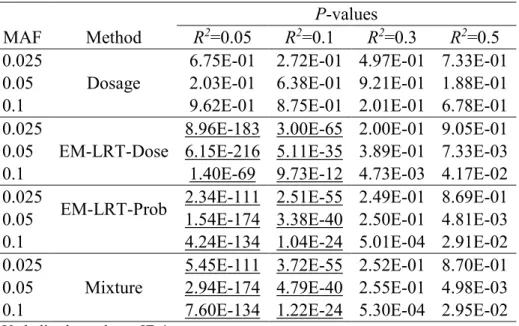
Type I Error Evaluation. We assess the validity of EM-LRT-Dose, Dosage, EM-LRT-

Prob, Mixture and gold-standard (based on true genotypes) under various combinations of R

and

MAF. Specifically, we simulate data sets each with 2,000 samples using pre-specified marker-

specific information R

and MAF, which allows us to generate genotype probabilities, dosages,

and true genotypes. Next, we simulate the trait values Y

according to the linear model for sample i with a set of pre-specified parameters, where i = 1, …, 2,000. For simplicity, we set

β

, β

, γ ^, σ

( ) ⁼ ( ^{1, 0,1,1} ) ^.

We repeat the simulation ten million times. For each simulated data set, we perform association testing based on the true genotypes (truth), as well as based on imputed data using the standard Dosage method, Mixture method, and our proposed EM-LRT-Prob and EM-LRT- Dose methods. The empirical type I error rate of each method is calculated as the proportion of observed p-values that fall below the specified significance level. In addition, we calculate the Spearman correlation between the observed and gold-standard (true genotype based) p-values.

Statistical Power Assessment. To evaluate the statistical power of different methods, we again simulate data sets each with 2,000 samples using a combination of marker-specific

information R

and MAF, and parameters ( β

, β

, γ ^, σ ) ⁼ ( ^{1, β}

^,1,1 ) ^{where β}

^∈ [ ^0,1.5 ] . We again repeat the simulations one million times. Similarly, for each simulated data set, we performed the same set of tests. The power of each method is calculated as the proportion of observed p-values that fall below the significance threshold α = 5 × 10

.

3.3 Results

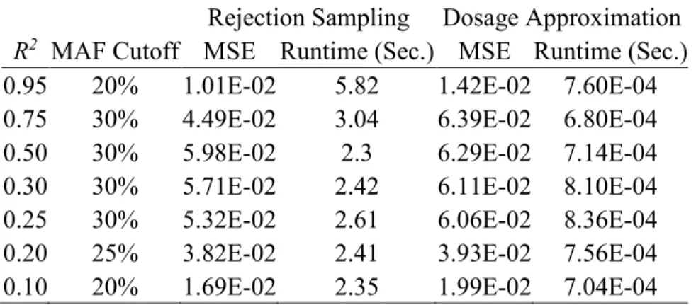
3.3.1 MAF Threshold

We used simulations to determine the MAF threshold specific to each R

such that the rejection sampling is advantageous (quantified by lower MSE in estimating f , the probability

of having one copy of the minor allele) over dosage approximation when exceeding the MAF threshold (Figure 1 and Table 1). We observed the two sampling methods have similar

2

such cases, we chose the simple dosage approximation method due to computational efficiency (Runtimes for rejection sampling and dosage approximation based on 2,000 samples are also shown). We also observed inferior performance (larger MSE) of both methods for low MAFs with intermediate R

values. Both can be explained by a combination of the imputation quality and the variation in f as a function of both imputation quality R

and MAF q. Specifically, we have Var( f ) = R

× 2q(1 – q) × (1 – 2q(1 – q)), which increases with MAF q as well as with R

. Low imputation quality R

coupled with low MAF leads to relatively little variation in f ,

rendering both sampling methods capable of estimating it relatively accurately. On the other hand, high imputation quality implies dosages close to true genotype values 0, 1, and 2, as well as f close to 0 or 1, thus allowing accurate inference of

f despite the larger variation in the

values of f across individuals. In the intermediate R

range, variation in f coupled with

imputation uncertainty makes inference challenging for both approaches.

3.3.2 Empirical Type I Error Simulation

As shown in Table 2 (at significance level 5E-02) and Table 3 (at significance level 5E- 05), all the methods have proper control of type I error across in the range of R

and MAF examined: 0.1 ≤ R

≤ 0.3 and 1% ≤ MAF ≤ 20%. Next, as shown in Figure 2, Spearman correlation with true p-values increases for every method when R

increases. The overall

correlation is low in the range of MAF and R

examined. This low correlation is expected given

the high level of imputation uncertainty and consistent with previous results (Zheng et al. 2011),

confirming that association inference is challenging with low frequency variants, or with variants

imputed with a high level of uncertainty. Although the absolute performance of all methods is

not particularly impressive, we observe that EM-LRT methods always show slightly higher

Spearman correlation than Dosage method especially when MAF is low, suggesting that the EM- LRT p-values better approach gold-standard p-values. When R

and MAF are high, all methods perform similarly (results not shown), consistent with results shown in literature (Zheng et al.

2011; Liu et al. 2013b).

3.3.3 Empirical Power Simulations

When R

and MAF are high, all methods have similar performance. In this chapter, we focus on scenarios where 0.1 ≤ R

≤ 0.3 and 1% ≤ MAF ≤ 20%. As shown in Figure 3, EM-LRT- Prob and Mixture methods are consistently the most powerful methods among all methods evaluated. However, these methods are not applicable in scenario II when only imputed dosages are available. It is thus valuable to notice that EM-LRT-Dose method approaches the statistical efficiency of EM-LRT-Prob, outperformng the standard Dosage method especially when R

or MAF is low. For example, when R

= 0.1 and MAF = 0.05, the power for EM-LRT-Prob, Mixture, EM-LRT-Dose and Dosage are 84.5%, 84.5%, 82.1%, and 61.4% under β

= 1.

3.4 Real Data Application

3.4.1 CLHNS

We applied the proposed EM-LRT methods as well as other existing methods to the Cebu Longitudinal Health and Nutrition Survey (CLHNS) study of 1,800 unrelated Filipino women.

We performed association analysis across chromosome 16, where we have previously identified the variants near CDH13 gene associated with plasma adiponectin level (Wu et al. 2010).

We conducted association testing with standardized adiponectin level measured in 2005 on a log scale as the quantitative trait and adjusted for age and BMI also measured in 2005.

Additionally, we excluded subjects from the analysis if they met one or more of the following

criteria: 1) subjects with adiponectin level missing or outside of the range mean +/– 4 standard deviations (n=19); 2) subjects carrying the R221S variant (n=53) (Croteau-Chonka et al. 2012);

and 3) subjects with missing age or BMI covariate information (n=20). In total, 1,717 subjects were tested for association with adiponectin level.

These 1,717 subjects were genotyped on the Affymetrix Genomewide Human SNP Array 5.0 GWAS chip (Lange et al. 2010) and also on the Illumina HumanExome Beadchip.

Specifically, we first established the truth by employing PLINK (Purcell et al. 2007) to perform association on the true genotypes separately, finding 10 true positives (p-value < 5×10

) on Affymetrix 5.0 and 5 on exome chip (with 2 overlapping). Next, to mimic a setting of low imputation quality, we masked all neighboring GWAS SNPs within 2kb of the 13 true positives before genotype imputation (22 SNPs were masked). Finally, we performed imputation using the MaCH imputation software (Li et al. 2010) using the ASN panel from the Phase I 1000 Genomes Project (March 2012 release, version 3) as reference. To evaluate the performance of the

proposed methods along with other alternatives, we used markers overlapping between the ASN reference panel and the exome chip, but not on the Affymetrix 5.0, at which we have both imputed genotypes and true genotypes (from exome chip genotyping). We then conducted association testing on the imputed genotypes (dosages or probabilities) using our proposed EM- LRT methods, Dosage, and Mixture method.

Figure 4 shows the Q-Q plot for the 1,135 SNPs on chromosome 16 with R

≤ 0.3 and

true p-value > 5×10

. Q-Q plots are used to assess the number and magnitude of observed

associations between tested SNPs and the trait under study, by comparing the observed –log

p-

values to what is expected under the null hypothesis of no association. Early departure from the

identity line suggests either that there is uncontrolled confouding leading to false positives (for

example, due to population stratification) or that a considerable proportion of SNPs are associated with the trait of interest (and thus not under the null distribution). Focusing on

variants with p-values > 5×10

based on experimental genotypes allowed us to examine the type I error empirically. Overall, this Q-Q plot suggests that all methods have proper control of type I error with all points falling within the 95% confidence bands with the exeption of one variant.

The single potential false positive, rs8045889 with a true p-value = 0.0148; R

= 0.0736; and MAF = 0.4271, was identified by Dosage, EM-LRT-Prob, and Mixture (EM-LRT-Dose has a borderline p-value of 0.0002). In addition, we observe overall deflation in the test statistics (observed larger p-values) of all methods when compared with truth. The median (mean) p- values are 0.6407, 0.5614, 0.5568 and 0.5568 (0.6075, 0.5552, 0.5512, and 0.5543) for Dosage, EM-LRT-Dose, EM-LRT-Prob and Mixture respectively, compared with the true median (mean) of 0.5008 (0.5009). The tendency towards large p-values is expected and driven by the loss of information due to imputation uncertainty.

While establishing the validity is crucial, we are more interested in the power to identify genuine associations. Table 4 tabulates p-values from all four methods together with the truth for variants with R

< 0.3 and true p-value < 5×10

. Although all variants reach the genome-wide significance threshold regardless of the method, we observed that EM-LRT-Dose or EM-LRT- Prob generated more significant p-values (and better approached truth in all cases) than the alternatives for five out of the six variants interrogated, suggesting power enhancement using our methods.

3.4.2 WHI

We have previously identified several variants associated with blood cell traits using

Americans with GWAS data from genome-wide Affymetrix 6.0 genotyping (Auer et al. 2012).

The samples are drawn from several cohorts including WHI, ARIC, CARDIA and JHS.

Association analyses were performed separately for WHI and CARe cohorts (ARIC, CARDIA and JHS) and subsequently meta-analyzed across the two. Due to the ascertainment of variants through whole exome sequencing, 56% of our analyzed variants had MAF < 5%.

Here, we use meta-analysis results from our previous study as a gold standard to define true positives and investigate the p-values in the WHI cohort using our EM-LRT-Dose and standard Dosage method, which had been adopted by the original study. We did not keep a copy of the posterior probabilities because of the large number of samples imputed and because standard analyses do not involve the posterior probabilities. Therefore, this is a real data example of scenario II. Table 5 presents all variants with MAF < 5% reported to reach genome-wide significant threshold in the original study, comparing p-values from our EM-LRT-Dose and the standard Dosage method. We notice that EM-LRT-Dose generated slightly more significant p- values at the associated variants in three out of the four tests performed. In one case (snp.177015 with white blood cell count [WBC]), the p-value from EM-LRT-Dose (p-value = 4.72×10

) reached the conventionally employed genome-wide significance threshold of 5×10

while that from Dosage was marginally genome-wide insignificant (p-value = 6.11×10

).

3.5 Discussion

It is crucial to take imputation uncertainty into consideration when performing

association testing. Existing methods have focused on common variants, which have been the

focus of the past wave of GWAS using HapMap-based imputation. With the deluge of next

generation sequencing data being generated, increasingly denser reference panels are allowing

imputation of a much larger number of variants, including an increasing number of relatively

rare or poorly imputed variants. It is thus highly warranted to re-visit potential strategies for post- imputation association analysis and to seek more powerful or efficient statistical methods.

In this chapter, we have proposed EM-LRT methods explicitly incorporating marker level imputation quality statistic into association tests. We considered two scenarios: when posterior probabilities of all potential genotypes are available and when only dosages are available. We evaluated the performance of the proposed methods along with existing alternatives using simulation studies and by application to real data sets.

In scenario I, our proposed EM-LRT-Prob demonstrated nearly identical performance as the Mixture model, which has been shown to be the best post-imputation association method particularly when imputation uncertainty is high (Zheng et al. 2011). While our EM-LRT-Prob effectively also fits a mixture model (therefore in terms of the underlying statistical model essentially the same as the Mixture method adopted in Zheng et al. 2011), we have proposed and implemented a much more computationally efficient algorithm to fit the model. Mixture method (Zheng et al. 2011) used R function optim() to find ML estimates. Technically, the optim() function uses numerical differentiation to obtain ML estimates based on the score function and Hessian matrix, which is considerably slower than our proposed EM algorithm. To quantify the computational efficiency, we conducted association testing on a CLHNS data set of 1,717 subjects and 13,801 SNPs, using EM-LRT-Prob and Mixture methods with the same starting values (the Mixture method tends to run even slower without using the suggested starting values).

We observed that the association tests required 279 seconds computing time and 0.91 GB RAM

for EM-LRT-Prob and 1,505 seconds computing time and 1.23 GB RAM for the Mixture method

on a 2.93 GHz Intel® Xeon® Processor X5670. Computing time scales linearly with sample size

for both EM-LRT-Prob and the Mixture method (Figure 5).