THE EXACT SOLUTION AND NUMERICAL IMPLEMENTATION OF THE FLAT ELECTRODYNAMIC PROCESS
14
0
0
Full text
(3)
(8)
(11)
(12)
(13)
(14)
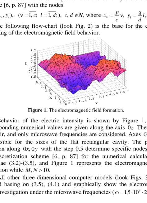
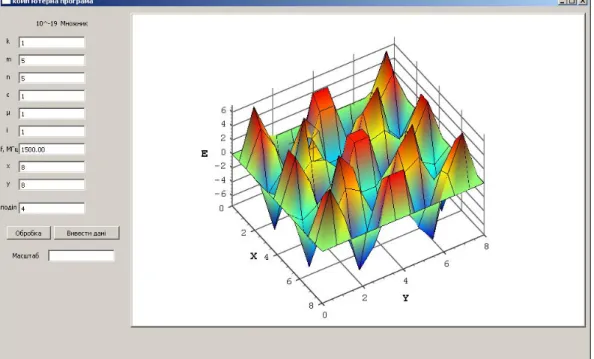
Figure

+3
Related documents