Coarse grained complexity for dynamic algorithms

warwick.ac.uk/lib-publications

Manuscript version: Author’s Accepted Manuscript

The version presented in WRAP is the author’s accepted manuscript and may differ from the

published version or Version of Record.

Persistent WRAP URL:

http://wrap.warwick.ac.uk/130123

How to cite:

Please refer to published version for the most recent bibliographic citation information.

If a published version is known of, the repository item page linked to above, will contain

details on accessing it.

Copyright and reuse:

The Warwick Research Archive Portal (WRAP) makes this work by researchers of the

University of Warwick available open access under the following conditions.

Copyright © and all moral rights to the version of the paper presented here belong to the

individual author(s) and/or other copyright owners. To the extent reasonable and

practicable the material made available in WRAP has been checked for eligibility before

being made available.

Copies of full items can be used for personal research or study, educational, or not-for-profit

purposes without prior permission or charge. Provided that the authors, title and full

bibliographic details are credited, a hyperlink and/or URL is given for the original metadata

page and the content is not changed in any way.

Publisher’s statement:

Please refer to the repository item page, publisher’s statement section, for further

information.

Coarse-Grained Complexity for Dynamic Algorithms

Sayan Bhattacharya

Danupon Nanongkai

Thatchaphol Saranurak

Abstract

To date, the only way to arguepolynomial lower boundsfor dynamic algorithms is viafine-grained complexity arguments. These arguments rely on strong assumptions aboutspecific problems such as the Strong Exponential Time Hypothesis (SETH) and the Online Matrix-Vector Multiplication Con-jecture (OMv). While they have led to many exciting dis-coveries, dynamic algorithms still miss out some benefits and lessons from the traditional “coarse-grained” approach that relates together classes of problems such as P and NP. In this paper we initiate the study of coarse-grained complexity the-ory for dynamic algorithms. Below are among questions that this theory can answer.

What if dynamic Orthogonal Vector (OV) is easy in the cell-probe model? A research program for provingpolynomial unconditional lower boundsfor dynamic OV in the cell-probe model is motivated by the fact that many conditional lower bounds can be shown via reductions from the dynamic OV problem (e.g. [Abboud, V.-Williams, FOCS 2014]). Since the cell-probe model is more powerful than word RAM and has historically allowed smaller upper bounds (e.g. [Larsen, Williams, SODA 2017; Chakraborty, Kamma, Larsen, STOC 2018]), it might turn out that dy-namic OV is easy in the cell-probe model, making this re-search direction infeasible. Our theory implies that if this is the case, there will be very interesting algorithmic conse-quences: If dynamic OV can be maintained in polylogarith-mic worst-case update time in the cell-probe model, then so are several important dynamic problems such ask-edge con-nectivity, (1 +)-approximate mincut, (1 +)-approximate matching, planar nearest neighbors, Chan’s subset union and 3-vs-4 diameter. The same conclusion can be made when we replace dynamic OV by, e.g., subgraph connectivity, single source reachability, Chan’s subset union, and 3-vs-4 diame-ter.

Lower bounds for k-edge connectivity via dy-namic OV?The ubiquity of reductions from dynamic OV raises a question whether we can prove conditional lower bounds for, e.g., k-edge connectivity, approximate mincut, and approximate matching, via the same approach. Our theory provides a method to refute such possibility (the so-called non-reducibility). In particular, we show that there are no “efficient” reductions (in both cell-probe and word RAM models) from dynamic OV tok-edge connectivity un-der an assumption about the classes of dynamic algorithms whose analogue in the static setting is widely believed. We are not aware of any existing assumptions that can play the same role. (The NSETH of Carmosino et al. [ITCS 2016] is the closest one, but is not enough.) To show similar

re-∗_{University of Warwick, UK.}

†_{KTH Royal Institute of Technology, Sweden.}

‡_{Toyota Technological Institute at Chicago, USA. Work}

par-tially done while at KTH Royal Institute of Technology.

sults for other problems, one only need to develop efficient randomizedverification protocolsfor such problems.

1 Introduction

In a dynamic problem, we first get an input instance for preprocessing, and subsequently we have to handle a sequence of updates to the input. For example, in the graph connectivity problem [35, 42], an n-node graph Gis given to an algorithm to preprocess. Then the algorithm has to answer whether G is connected or not after each edge insertion and deletion to G. (Some dynamic problems also consider queries. (For example, in the connectivity problem an algorithm may be queried whether two nodes are in the same connected component or not.) Since queries can be phrased as input updates themselves, we will focus only on updates in this paper. Algorithms that handle dynamic problems are known as dynamic algorithms. The preprocessing time of a dynamic algorithm is the time it takes to handle the initial input, whereas the worst-case update time of a dynamic algorithm is the

maximumtime it takes to handle any update. Although dynamic algorithms are also analyzed in terms of their

amortized update times, we emphasize that the results in this paper deal only with worst-case update times. A holy grail for many dynamic problems – especially those concering dynamic graphs under edge deletions and insertions – is to design algorithms withpolylogarithmic update times. From this perspective, the computational status of many classical dynamic problems still remain widely open.

(even with randomization) remains polynomial [68]. (iii) For dynamic k-edge connectivity with k ≥ 3, the best update time – amortization and randomization allowed – suddenly jumps to ˜O(√n) where ˜O hides polylogarithmic terms. Indeed, it is a major open problem to maintain a (1 + )-approximation to the value of global minimum cut in a dynamic graph in polylogarithmic update time [68]. Doing so for k-edge connectivity with k = O(logn) is already sufficient to solve the general case.

Other dynamic problems that are not known to admit polylogarithmic update times include approx-imate matching, shortest paths, diameter, max-flow, etc. [68, 61]. Thus, it is natural to ask: can one ar-gue that these problems do not admit efficient dynamic algorithms?

A traditionally popular approach to answer the question above is to use information-theoretic argu-ments in thebit-probe/cell-probe model. In this model of computation, all the operations are freeexcept memory accesses. (In more details, the bit-probe model con-cerns the number of bits accessed, while the cell-probe model concerns the number of accessed cells, typically of logarithmic size.) Lower bounds via this approach are usually unconditional, meaning that it does not rely on any assumption. Unfortunately, this approach could only give small lower bounds so far; and getting a super-polylogarithmic lower bound for anynatural dy-namic problem is an outstanding open question is this area [46].

More recent advances towards answering this ques-tion arose from a new area called fine-grained complex-ity. While traditional complexity theory (henceforth we refer to it ascoarse-grained complexity) focuses on classi-fying problems based on resources and relating together resulting classes (e.g. P and NP), fine-grained com-plexity gives us conditional lower bounds in the word RAM model based on various assumptions about spe-cific problems. For example, assumptions that are par-ticularly useful for dynamic algorithms are the Strong Exponential Time Hyposis (SETH), which concerns the running time for solving SAT, and the Online Matrix-Vector Multiplication Conjecture (OMv), which con-cerns the running time of certain matrix multiplication methods (more at, e.g., [57, 3, 34]). In sharp contrast to cell-probe lower bounds, these assumptions often lead to polynomial lower bounds in the word RAM model, many of which are tight.

While the fine-grained complexity approach has led to many exciting lower bound results, there are a num-ber of traditional results in the static setting that seem to have no analogues in the dynamic setting. For ex-ample, one reason that makes the P 6= N P

assump-tion so central in the static setting is that proving and disproving it will both lead to stunning consequences: If the assumption is false then hundreds of problems in NP and bigger complexity classes like the polyno-mial hierarchy (PH) admit efficient algorithms; other-wise the situation will be the opposite.1 In contrast, we do not see any immediate consequence to dynamic algo-rithms if someone falsified SETH, OMv, or any other as-sumptions.2 As another example, comparing complex-ity classes allows us to speculate on various situations such as non-reducibility (e.g. [4,43, 19]), the existence of NP-intermediate problems [44] and the derandom-ization possibilities (e.g. [40]). (See more in Section4.) We cannot anticipate results like these in the dynamic setting without the coarse-grained approach, i.e. by considering analogues of P, NP, BPP and other com-plexity classes that are defined based on computational resources.

Our Main Contributions. We initiate a system-atic study of coarse-grained complexity theory for dy-namic problems in the bit-probe/cell-probe model of computation. We now mention a couple of concrete im-plications that follow from this study.

Consider the dynamic Orthogonal Vector (OV) problem (see Definition2.4). Lower bounds conditional on SETH for many natural problems (e.g. Subgraph connectivity, ST-reachability, Chan’s subset union, 3-vs-4 Diameter) are based on reductions from dynamic OV [3]. This suggests two research directions: (I) Prove strongunconditionallower bounds for many nat-ural problems in one shot by proving a polynomial cell-probe lower bound for dynamic OV. (II) Prove lower bounds conditional on SETH for the family of connec-tivity problems mentioned in the previous page via re-ductions (in the word RAM model) from dynamic OV. Below are some questions about the feasibility of these research directions that our theory can answer. We are not aware of any other technique in the existing litera-ture that can provide similar conclusions.

(I) What if dynamic OV is easy in the cell-probe model? For the first direction, there is a risk that dynamic OV might turn out to admit a polylogarithmic update time algorithm in the cell-probe model. This is

1_{For further consequences see, e.g., [1,20,21] and references} therein.

because lower bounds in the word RAM model do not necessarily extend to the cell-probe model. For example, it was shown by Larsen and Williams [47] and later by Chakraborty et al [17] that the OMv conjecture [34] is false in the cell-probe model.

Will all the efforts be wasted if dynamic OV turns out to admit polylogarithmic update time in the cell-probe model? Our theory implies that this will also lead to a very interesting algorithmic consequence: If dynamic OV admits polylogarithmic update time in the cell-probe model, so do several important dynamic prob-lems such as k-edge connectivity, (1 +)-approximate mincut, (1 +)-approximate matching, planar nearest neighbors, Chan’s subset union and 3-vs-4 diameter. The same conclusion can be made when we replace dy-namic OV by, e.g., subgraph connectivity, single source reachability, Chan’s subset union, and 3-vs-4 diameter (see Theorem 2.1). Thus, there will be interesting con-sequences regardless of the outcome of this line of re-search.

Roughly, we reach the above conclusions by proving in the dynamic setting an analogue of the fact that if P=NP (in the static setting), then the polynomial hierarchy (PH) collapses. This is done by carefully defining the classes Pdy, NPdy and PHdy as dynamic analogues of P, NP, and PH, so that we can prove such statements, along with NPdy-completeness and NPdy -hardness results for natural dynamic problems including dynamic OV. We sketch how to do this in Sections2,5.

(II) Lower bounds for k-edge connectivity via dynamic OV? As discussed above, whether dynamic

k-edge connectivity admits polylogarithmic update time for k∈[3, O(logn)] is a very important open question. There is a hope to answer this question negatively via reductions (in the word RAM model) from dynamic OV. Our theory provides a method to refute such a possibility (the so-called non-reducibility). First, note that any reduction from dynamic OV in the word RAM model will also hold in the (stronger) cell-probe model. Armed with this simple observation, we show that there are no “efficient” reductions from dynamic OV to k-edge connectivity under an assumption about the complexity classes for dynamic problems in the cell-probe model, namely PHdy 6⊆ AMdy ∩coAMdy (see Theorem 2.2). We defer defining the classes AMdy and coAMdy, but note two things. (i) Just as the classes AM and coAM (where AM stands for Arthur-Merlin) extend NP in the static setting, the classes AMdy and coAMdy extend the classNPdy in a similar manner. (ii) In the static setting it is widely believed that PH6⊆AM

∩ coAM because otherwise the PH collapses. Roughly, the phrase “efficient reduction” from problemsX toY

refers to a way of processing each update for problemX

by quickly feeding polylogarithmic number of updates as input to an algorithm for Y. All reductions from dynamic OV in the literaturethat we are aware of are efficient reductions.

Remark: We define our complexity classes in the cell-probe model, whereas the reductions from dynamic OV are in the word RAM model. This does not make any difference, however, since any reduction in the word RAM reduction continues to have the same guarantees in the (stronger) cell-probe model.

To show a similar non-reducibility result for any problem X, one needs to prove that X ∈ AMdy ∩

coAMdy, which boils down to developing efficient ran-domized verification protocols for such problems. We explain this in more details in Section2.

We are not aware of any existing assumptions that can lead the same conclusion as above. To our knowledge, the only conjecture that can imply results of this nature is the Nondeterministic Strong Exponential Time Hypothesis (NSETH) of [16]. However, it needs a stronger property of k-edge connectivity that is not yet known to be true. (In particular, Theorem 2.2 follows from the fact that k-edge connectivity is in AMdy∩coAMdy. To use NSETH, we need to show that it is inNPdy∩coNPdy.) Moreover, even if such a property holds it would only rule out deterministic reductions since NSETH only holds for deterministic algorithms.

Paper Organization. In Section 2, we explain our contributions in details, including the conclusions above and beyond. We discuss related works and future directions in Sections3and4. An overview of our main NPdy-completeness proof is in Section5.

2 Our Contributions in Details

We show that coarse-grained complexity results similar to the static setting can be obtained for dynamic prob-lems in the bit-probe/cell-probe model of computation,3

provided the notion of “nondeterminism” is carefully de-fined. Recall that the cell-probe model is similar to the word RAM model, but the time complexity is measured by the number of memory reads and writes (probes); other operations are free. Like in the static setting, we only considerdecisiondynamic problems, meaning that the output after each update is either “yes” or “no”. Note the following remarks.

• Readers who are familiar with the traditional com-plexity theory may wonder why we do not consider the Turing machine. This is because the Turing ma-chine is not suitable for implementing dynamic

gorithms, since we cannot access an arbitrary tape location in O(1) time. There is no efficient algo-rithm even for a basic data structure like the binary search tree.

• Our results for decision problems extend naturally to promised problems which are useful when we discuss approximation algorithms. We do not dis-cuss promised problems here to keep the disdis-cussions simple.

• Readers who are familiar with the oblivious ad-versaries assumption for randomized dynamic al-gorithms may wonder if we consider this assump-tion here. This assumpassump-tion plays no role for de-cision problems, since an algorithm that is correct with high probability (w.h.p.) under this assump-tion is also correct w.h.p. without the assumpassump-tion (in other words, its output reveals no information about its randomness). Because of this, we do not discuss this assumption in this paper.

We start with our main results which can be ob-tained with appropriate definitions of complexity classes Pdy _{⊆ NP}dy _{⊆ PH}dy _{for dynamic problems: These} classes are described in details later. For now they should be thought of as analogues of the classes P, NP and PH (polynomial hierarchy).

Theorem 2.1. (Pdy vs. NPdy) Below, the phrase “effi-cient algorithms” refers to dynamic algorithms that are deterministic and require polylogarithmic worst-case up-date time and polynomial space to handle a polynomial number of updates in the bit-probe/cell-probe model.

1. The dynamic orthogonal vector (OV) problem is “NPdy-complete”, and there are a number of dy-namic problems that are “NPdy-hard” in the sense that ifPdy6=NPdy, then they admitnoefficient al-gorithms. These problems include decision versions of Subgraph connectivity, ST-reachability, Chan’s subset union, and 3-vs-4 Diameter (see Tables 2,3 for more).

2. If Pdy = NPdy then Pdy = PHdy, meaning that all problems in PHdy (which contains the class NPdy) admit efficient algorithms. These problems include decision versions of k-edge Connectivity,

(1 +)-approximate Matching,4 _{(1 +)-approximate}

4_{Technically speaking, (1 + )-approximate matching is a}

promisedorgapproblem in the sense that for some input instance all answers are correct. It is inpromise−PHdy which is bigger than PHdy. We can make the same conclusion for promised problems: IfPdy =NPdy, then all problems inpromise−PHdy

admit efficient algorithms.

mincut, Planar nearest neighbors, Chan’s subset union and 3-vs-4 Diameter (see Tables 2, 4 for more).

Thus, proving or disproving Pdy 6=NPdy will both lead to interesting consequences: If Pdy 6= NPdy, then many dynamic problems do not admit efficient algo-rithms. Otherwise, ifPdy =NPdy, then many problems admit efficient algorithms which are not known or even believed to exist.

Remark: We can obtain similar results in the word-RAM model, but we need a notion of “efficient algorithms” that is slightly non-standard in that a quasi-polynomial preprocessing time is allowed. (In contrast, all our results hold in the standard cell-probe setting.) We postpone discussing word-RAM results to later in the paper to avoid confusions.

As another showcase, our study implies a way to shownon-reducibility, like below.

Theorem 2.2. Assuming PHdy 6⊆ AMdy ∩ coAMdy, the k-edge connectivity problem cannot be NPdy-hard. Consequently, there is no “efficient reduction” from the dynamic Orthogonal Vector (OV) problem to k-edge connectivity.

From the discussion in Section1, recall that thek -edge connectivity problem is currently known to admit a polylogarithmic amortized update time algorithm for

k ≤2, and aO(√npolylog(n)) update time algorithm fork∈[3, O(logn)].It is a very important open problem whether it admits polylogarithmic worst-case update time. Theorem 2.2 rules out a way to prove lower bounds and suggest that an efficient algorithm might exist.

A more important point beyond the k-edge con-nectivity problem is that one can prove a similar re-sult for any dynamic problemX by showing that X ∈

AMdy ∩coAMdy or, even better, X ∈ NPdy ∩coNPdy. See Section4 for some candidate problems forX. This is easier than showing a dynamic algorithm forX itself. Thus, this method is an example of the by-products of our study that we expect to be useful for developing algorithms and lower bounds for dynamic problems in future. See Section 2.4 for more details. As noted in Section 1, we are not aware of any existing technique that is capable of deriving a non-reducibility result of this kind.

2.1 Defining the Complexity Classes Pdy _and NPdy Class Pdy_{. We start with P}dy_{, the class of} dynamic problems that admit “efficient” algorithms in the cell-probe model. For any dynamic problem, define its update size to be the number of bits needed to describe each update. Note that we have not yet defined what dynamic problems are formally. Such a definition is needed for a proper, rigorous description of our complexity classes, and can be found in the full version of the paper. For an intuition, it suffices to keep in mind that most dynamic graph problems – where each update is an edge deletion or insertion – have logarithmic update size (since it takesO(logn) bits to specify an edge in an n-node graph).

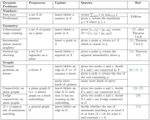
Definition 2.1. (Pdy; brief) A dynamic problem with polylogarithmic update size is in Pdy _{if it admits a} deterministic algorithm with polylogarithmic worst-case update time for handling a sequence of polynomially many updates.

Examples of problems in Pdy include connectivity on plane graphs and predecessor; for more, see Table1. Note that one can definePdy more generally to include problems with larger update sizes. Our complexity results hold even with this more general definition. However, since our results are most interesting for problems with polylogarithmic update size, we focus on this case in this paper to avoid cumbersome notations.

Class NPdy and nondeterminism with re-wards. Next, we introduce our complexity classNPdy. Recall that in the static setting the class NP consists of the set of problems that admit efficiently verifiable proofs or, equivalently, that are solvable in polynomial time by a nondeterministic algorithm. Our notion of nondeterminism is captured by the proof-verification definition where, after receiving a proof, the verifier does not only output YES/NO, but also a reward, which is supposed to be maximized at every step.

Before definingNPdymore precisely, we remark that the notion of reward is a key for ourNPdy-completeness proof. Having the constraint about rewards potentially makes NPdy contains less problems. Interestingly, all natural problems that we are aware of remains inNPdy even with this constraint. This might not be a big surprise, when it is realized that in the static setting imposing a similar constraint about the reward doesnot

make the class (static) NP smaller; see more discussions below. We now define NPdy more precisely.

Definition 2.2. (NPdy; brief) A dynamic problemΠ

with polylogarithmic update size is in NPdy if there is a verifier that can do the following over a sequence of polynomially many updates: (i) after every update, the verifier takes the update and a polylogarithmic-sizeproof

as an input, and (ii) after each update, the verifier outputs in polylogarithmic time a pair (x, y), where

x ∈ {Y ES, N O}and y is an integer (representing a reward) with the following properties.5

1. If the current input instance is an YES-instance and the verifier has so far always received a proof that maximizes the reward at every step, then the verifier outputs x=Y ES.

2. If the current input instance is a NO-instance, then the verifier outputs x=N O regardless of the sequence of proofs it has received so far.

To digest the above definition, first consider the

static setting. One can redefine the class NP for static problems in a similar fashion to Definition 2.2 by removing the preprocessing part and letting the only update be the whole input. Let us refer to this new (static) complexity class as “reward-NP”. To show that a static problem is in reward-NP, a verifier has to output some reward in addition to the YES/NO answer. Since usually a proof received in the static setting is a solution itself, a natural choice for reward is the cost of the solution (i.e., the proof). For example, a “proof” in the maximum clique problem is a big enough clique, and in this case an intuitive reward would be the size of the clique given as a proof. Observe that this is sufficient to show that max clique is in reward-NP. In fact, it turns out thatin the static setting the complexity classes NP and reward-NP are equal. (Proof sketch: Let Π be any problem in the original static NP and V

be a corresponding verifier. We extend V to V0 which outputs x = Y ES/N O as V and outputs y = 1 as a reward if x=Y ES andy= 0 otherwise. It is not hard to check thatV0 satisfies conditions in Definition2.2.)

To further clarify Definition 2.2, we now consider examples of some well-known dynamic problems that happen to be inNPdy.

Example 1. (Subgraph Detection) In the

dy-namic subgraph detection problem, an n-node and

k-node graphs GandH are given at the preprocessing, for some k = polylog(n). Each update is an edge insertion or deletion in G. We want an algorithm to output YES if and only ifG hasH as a subgraph.

This problem is in NPdy due to the following ver-ifier: the verifier outputs x = Y ES if and only if the proof (given after each update) is a mapping of the edges inH to the edges in a subgraph of Gthat is isomorphic to H. With output x=Y ES, the verifier gives reward

y = 1. With output x=N O, the verifier gives reward

5_{Later in the paper, we use x = 1 andx = 0 to represent}

y = 0. Observe that the proof is of polylogarithmic size (sincek= polylog(n)), and the verifier can calculate its outputs (x, y) in polylogarithmic time. Observe further that the properties stated in Definition2.2are satisfied: if the current input instance is a YES-instance, then the reward-maximizing proof is a mapping between H and the subgraph of Gisomorphic toH, causing the verifier to output x=Y ES; otherwise, no proof will make the verifier outputx=Y ES.

The above example is in fact too simple to show the strength of our definition that allows NPdy to include many natural problems (for one thing, y is simply 0/1 depending onx). The next example demonstrates how the definition allows us to develop more sophisticated verifiers for other problems.

Example 2. (Connectivity) In the dynamic

con-nectivity problem, an n-node graph G is given at the preprocessing. Each update is an edge insertion or dele-tion inG. We want an algorithm to output YES if and only ifGis connected.

This problem is in NPdy due to the following veri-fier. After every update, the verifier maintains a forest

F of G. A proof (given after each update) is an edge insertion to F or an ⊥ symbol indicating that there is no update to F. It handles each update as follows.

• After an edge e is inserted into G, the verifier checks if e can be inserted into F without creating a cycle. This can be done in O(polylog(n)) time using a link/cut tree data structure [65]. It outputs reward y= 0. (No proof is needed in this case.)

• After an edgeeis deleted fromG, the verifier checks if F contains e. If not, it outputs reward y = 0

(no proof is needed in this case). If eis in F, the verifier reads the proof (given aftereis deleted). If the proof is⊥it outputs reward y= 0. Otherwise, let the proof be an edge e0. The verifier checks if

F0 = F \ {e} ∪ {e0} is a forest; this can be done in O(polylog(n)) time using a link/cut tree data structure [65]. If F0 is a forest, the verifier sets

F ← F0 _{and outputs reward y = 1; otherwise, it}

outputs rewardy=−1.

After each update, the verifier outputsx=Y ES if and only ifF is a spanning tree ofG.

Observe that if the verifier gets a proof that maxi-mizes the reward after every update, the forest F will always be a spanning forest (since inserting an edge

e0 to F has higher reward than giving ⊥ as a proof ). Thus, the verifier will always outputx=Y ES for YES-instances in this case. It is not hard to see that the verifier never outputs x = Y ES for NO-instances, no matter what proof it receives.

In short, a proof for the connectivity problem is the maximal spanning forest. Since such proof is too big to specify and verify after every update, our definition allows such proof to be updated over input changes. (This is as opposed to specifying the densest subgraph from scratch every time as in Example1.) Allowing this is crucial for most problems to be in NPdy, but create difficulties to proveNPdy-completeness. We remedy this by introducing rewards.

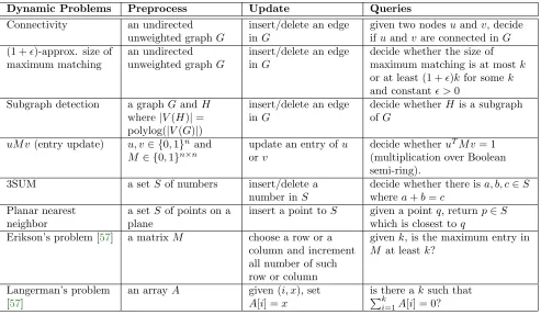
Note that if there is no reward in Definition 2.2, then it is even easier to show that dynamic connectivity and other problems are in NPdy. Having an additional constraint about rewards potentially makes less prob-lems verifiable. Luckily, all natural probprob-lems that we are aware of that were verifiable without rewards re-main verifiable with rewards. Problems inNPdy include decision/gap versions of (1 +)-approximate matching, planar nearest neighbor, and dynamic 3SUM; see Ta-ble 2 for more. The concept of rewards (introduced while defining the class NPdy) will turn to be crucial when we attempt to show the existence of a complete problem inNPdy. See Section2.2and Section5for more details.

It is fairly easy to show that Pdy _⊆NPdy_{, and we} conjecture that Pdy _6=NPdy_.

Previous nondeterminism in the dynamic setting. The idea of nondeterministic dynamic algo-rithms is not completely new. This was considered by Husfeldt and Rauhe [39] and their follow-ups [58, 56, 75, 45, 69], and has played a key role in proving cell-probe lower bounds in some of these papers. As dis-cussed in [39], although it is straightforward to define a nondeterministic dynamic algorithm as the one that can make nondeterministic choices to process each up-date and query, there are different ways to handle how nondeterministic choices affect the states of algorithms which in turns affect how the algorithms handle future updates (called the “side effects” in [39]). For example, in [39] nondeterminism is allowed only for answering a query, which happens to occur only once at the very end. In [58], nondeterministic query answering may happen throughout, but an algorithm is allowed to write in the memory (thus change its state) only if all nondetermin-istic choices lead to the same memory state.

however, we distinct different choices by giving them different rewards. These differences allow us to include more problems to our NPdy (we do not know, for ex-ample, if dynamic connectivity admits nondeterministic algorithms according to previous definitions).

2.2 NPdy-Completeness Here, we sketch the idea behind our NPdy-completeness and hardness results. We begin by introducing a problem is called dynamic narrow DNF evaluation problem (in short, DNFdy), as follows.

Definition 2.3. (DNFdy; informally) Initially, we have to preprocess (i) an m-clause n-variable DNF formula6 where each clause contains O(polylog(m))

literals, and (ii) an assignment of (boolean) values to the variables. Each update changes the value of one variable. After each update, we have to answer whether the DNF formula is true or false.

It is fairly easy to see that DNFdy ∈ NPdy: After each update, if the DNF formula happens to be true, then the proof only needs to point towards one satisfied clause, and the verifier can quickly check if this clause is satisfied or not since it contains only O(polylog(m)) literals. Surprisingly, it turns out that this is also a complete problem in the classs NPdy.

Theorem 2.3. (NPdy-completeness of DNFdy) The DNFdy problem isNPdy-complete. This means that DNFdy ∈NPdy, and if DNFdy ∈Pdy_{, thenP}dy _=NPdy

.

To start with, recall the following intuition for proving NP-completeness in the static setting (e.g. [6, Section 6.1.2] for details): Since Boolean circuits can simulate polynomial-time Turing machine computation (i.e. P ⊆ P/poly), we view the computation of the verifier V for any problem Π in NP as a circuit C. The input of C is the proof that V takes as an input. Then, determining whether there is an input (proof) that satisfies this circuit (known asCircuitSAT) is NP-complete, since such information will allow the verifier to find a desired proof on its own. Attempting to extend this intuition to the dynamic setting might encounter the following roadblocks.

1. Boolean circuits cannot efficiently simulate algo-rithms in the RAM model without losing a linear factor in running time.Furthermore, an alternative such as circuits with “indirect addressing” gates seems useless, because this complex gate makes the model more complicated. This makes it more diffi-cult to prove NPdy-hardness.

6_{Recall that a DNF formula is in the formC}

1∨ · · ·∨Cm, where each “clause”Ciis a conjunction (AND) of literals.

2. Since the verifier has to work through several up-dates in the dynamic setting, the YES/NO out-put from the verifier alone is insufficient to indicate proofs that can be useful forfutureupdates. For ex-ample, suppose that in Example2the connectivity verifier is allowed to output onlyx∈ {Y ES, N O}, and we get rid of the concept of a reward. Con-sider a scenario where an edge e (which is part of

F) gets deleted from G, and G was disconnected even before this deletion. In this case, the veri-fier can indicate no difference between having e0

(i.e. finding a reconnecting edge) and⊥(i.e. doing nothing) as a proof (because it has to outputx= 0 in both cases). Having e0 as a proof, however, is more useful for the future, since it helps maintain a spanning forest.

It so happens that we can solve (ii) if the verifier additionally outputs an integer y as a reward. Asking more from the verifier makes less problems verifiable (thus smaller NPdy). Luckily, all natural problems we are aware of that were verifiable without rewards remain verifiable with rewards!

To solve (i), we use the fact that in the cell-probe model a polylogarithmic-update-time algorithm can be modeled by a polylogarithmic-depth decision assignment tree[49], which naturally leads to a complete problem about a decision tree (we leave details here; see Section 5 for more). It turns out that we can reduce from this problem to DNFdy (Definition 2.3); the intuition being that each bit in the main memory corresponds to a boolean variable and each root-to-leaf path in the decision assignment tree can be thought of as a DNF clause. The only downside of this approach is that a polylogarithmic-depth decision tree has quasi-polynomial size. A straightforward reduction would cause quasi-polynomial space in the cell-probe model. By exploiting the special property of DNFdy and the fact that the cell-probe model only counts the memory access, we can avoid this space blowup by “hardwiring” some space usage into the decision tree and reconstruct some memory when needed.

The fact that the DNFdyproblem isNPdy-complete (almost) immediately implies that many well-known dynamic problems areNPdy-hard. To explain why this is the case, we first recall the definition of the dynamic sparse orthogonal vector (OVdy) problem.

Definition 2.4. (OVdy) Initially, we have to prepro-cess a collection of m vectors V = {v1, . . . , vm} where each vj ∈ {0,1}n, and another vector u ∈ {0,1}n. It is guaranteed that each vj ∈ {0,1}n has at most

up-date, we have to answer if there is a vector v ∈V that is orthogonal tou(i.e., if uT_{v= 0).}

The key observation is that the OVdy problem is equivalent to the DNFdy problem, in the sense that OVdy ∈ Pdy iff DNFdy ∈ Pdy. The proof is relatively straightforward (the vectors vj and the individual entries of u respectively correspond to the clauses and the variables in DNFdy), and we defer it to the full version of the paper. In [3], Abboud and Williams show SETH-hardness for all of the problems in Table3. In fact, they actually show a reduction from OVdy to these problems. Therefore, we immediately obtain the following result.

Corollary 2.1. All problems in Table 3 are NPdy -hard.

2.3 Dynamic Polynomial Hierarchy By intro-ducing the notion of oracles, it is not hard to extend the class NPdy into polynomial-hierarchy for dynamic problems, denoted by PHdy. Roughly, PHdy is the union of classes Σdy_i and Πdy_i , where (i) Σdy₁ = NPdy, Πdy₁ =coNPdy, and (ii) we say that a dynamic problem is in class Σdy_i (resp. Πdy_i ) if we can show that it is in NPdy (resp. coNPdy) assuming that there are efficient dynamic algorithms for problems in Σi−1. The details appear in the full version of the paper.

Example 3. (k- and (<k)-edge connectivity) In the dynamic k-edge connectivity problem, an n-node graph G= (V, E) and a parameter k =O(polylog(n))

is given at the time of preprocessing. Each update is an edge insertion or deletion inG. We want an algorithm to output YES if and only if Ghas connectivityat least

k, i.e. removing at mostk−1 edges willnotdisconnect

G. We claim that this problem is in Πdy₂ . To avoid dealing with coNPdy, we consider the complement of this problem called dynamic (¡k)-edge connectivity, where x =Y ES if and only if G has connectivity less thank. We show that (¡k)-edge connectivity is in Σdy₂ .

We already argued in Example 2 that dynamic connectivity is in NPdy = Σdy₁ . Assuming that there exists an efficient (i.e. polylogarithmic-update-time) algorithm A for dynamic connectivity, we will show that (¡k)-edge connectivity is in NPdy. Consider the following verifier V. After every update in G, the verifier V reads a proof that is supposed to be a set

S ⊆E of at mostk−1 edges. V then sends the update to A and also tellsA to delete the edges in S from G. If A says that G is not connected at this point, then the verifier V outputs x = Y ES with reward y = 1; otherwise, the verifier V outputs x=N O with reward

y = 0. Finally, V tells A to add the edges inS back in

G.

Observe that if G has connectivity less than k and the verifier always receives a proof that maximizes the reward, then the proof will be a set of edges disconnecting the graph and V will answer YES. Otherwise, no proof can make V answer YES. Thus the dynamic (¡k)-edge connectivity problem is in NPdy if A exists. In other words, the problem is inΣdy₂ .

By arguments similar to the above example, we can show that other problems such as Chan’s subset union and small diameter are inPHdy; see Table4 for more.

The theorem that plays an important role in our main conclusion (Theorem2.1) is the following.

Theorem 2.4. If Pdy =NPdy, thenPHdy =Pdy.

To get an idea how to proof the above theorem, observe that ifPdy _=NPdy

, thenAin Example3exists and thus dynamic (¡k)-edge connectivity are in Σdy₁ = NPdyby the argument in Example2; consequently, it is in Pdy_{! This type of argument can be extended to all} other problems inPHdy.

2.4 Other Results and Remarks In previous sub-sections, we have stated two complexity results, namely NPdy-completeness/hardness and the collapse of PHdy when Pdy _=NPdy_{. With right definitions in place, it is} not a surprise that more can be proved. For example, we obtain the following results:

1. IfNPdy ⊆coNPdy, then PHdy=NPdy∩coNPdy.

2. If NPdy ⊆AMdy∩coAMdy, then PHdy ⊆AMdy ∩

coAMdy.

Here, coNPdy, AMdy, and coAMdy are analogues of complexity classes coNP, AM, and coAM. The details appear in the full version of the paper.

While the coarse-grained complexity results in this paper are mostly resource-centric (in contrast to fine-grained complexity results that are usually centered around problems), we also show that this approach is helpful for understanding the complexity of specific problems as well, in the form of non-reducibility. In particular, the following results are shown in the full version of the paper:

1. Assuming PHdy 6= NPdy∩coNPdy, the two state-mentscannothold at the same time.

(b) One of the following problems is NPdy -hard: approximate minimum spanning for-est (MSF), d-weight MSF,bipartiteness, and

k-edge connectivity.

2. k-edge connectivity is in AMdy∩coAMdy. Conse-quently, assuming PHdy6⊆AMdy∩coAMdy,k-edge connectivity cannot beNPdy-hard.

Note that both PH 6= NP ∩ coNP and PH 6⊆

AM∩coAMare widely believed in the static setting since refuting them means collapsingPH. While we can show thatPHdywould also collapse ifPHdy=NPdy∩coNPdy, it remains open whether this is the case for PHdy ⊆

AMdy∩coAMdy; in particular isPHdy⊇AMdy∩coAMdy? When a problem Y cannot be NPdy-hard, there is no efficient reduction from anNPdy-hard problemX to

Y, where an efficient reduction is roughly to a way to handle each update for problemX by making polyloga-rithmic number of updates to an algorithm forY (such reduction would makeY anNPdy-hard problem). Con-sequently, this rules out efficient reductions from dy-namic OV, since it is NPdy-complete. As a result, this rules out a common way to prove lower bounds based on SETH, since previously this was mostly done via reduc-tions from dynamic OV [3]. (A lower bound for dynamic diameter is among a very few exception [3].)

2.5 Relationship to Fine-Grained Complexity As noted earlier, it turns out that the dynamic OV prob-lem is NPdy-complete. Since most previous reductions from SETH to dynamic problems (in the word RAM model) are in fact reductions from dynamic OV [3], and since any reduction in the word RAM model applies also in the (stronger) cell-probe model, we get many NPdy -hardness results for free. In contrast, our results above imply that the following two statements are equivalent: (i) “problem Π cannot beNPdy-hard” and (ii) “there is no efficient reduction from dynamic OV to Π”, where “efficient reductions” are reduction that only polynomi-ally blow up the instance size (all reductions in [3] are efficient). In other words, we may not expect reduc-tions from SETH that are similar to the previous ones fork-edge connectivity, bipartiteness, etc.

Finally, we emphasize that the coarse-grained ap-proach should be viewed as a complement of the fine-grained approach, as the above results exemplify. We do not expect to replace results from one approach by those from another.

2.6 Complexity classes for dynamic problems in the word RAM model As an aside, we managed to define complexity classes and completeness results for dynamic problems in the word RAM model as well. We

refer toPdy _andNPdy

as RAM−Pdy andRAM−NPdy in the word-RAM model. One caveat is that for tech-nical reasons we need to allow for quasipolynomial pre-processing time and space while defining the complexity classes RAM−Pdy and RAM−NPdy. We discuss this in more details in the full version of the paper.

3 Related Work

There are several previous attempts to classify dynamic problems. First, there is a line of works called “dynamic complexity theory” (see e.g. [24, 70, 63]) where the general question asks whether a dynamic problem is in the class called DynFO. Roughly speaking, a problem is in DynFO if it admits a dynamic algorithm expressible by a first-order logic. This means, in particular, that given an update, such algorithm runs in O(1) parallel time, but might take arbitrary poly(n) works when the input size is n. A notion of reduction is defined and complete problems of DynFO and related classes are proven in [36, 70]. However, as the total work of algorithms from this field can be large (or even larger than computing from scratch using sequential algorithms), they do not give fast dynamic algorithms in our sequential setting. Therefore, this setting is somewhat irrelevant to our setting.

Second, a problem called the circuit evaluation

problem has been shown to be complete in the following sense. First, it is in P (the class of static problems). Second, if the dynamic version of circuit evaluation problem, which is defined as DNFdy where a DNF-formula is replaced with an arbitrary circuit, admits a dynamic algorithm with polylogarithmic update time, then for any static problemL∈P, a dynamic version of

Lalso admits a dynamic algorithm with polylogarithmic update time. This idea is first sketched informally since 1987 by Reif [60]. Miltersen et al. [50] then formalized this idea and showed that other P-complete problems listed in [51, 32] also are complete in the above sense.7

The drawback about this completeness result is that the dynamic circuit evaluation problem is extremely difficult. Similar to the case for static problems that reductions fromEXP-complete problems to problems in NP are unlikely, reductions from the dynamic circuit evaluation problem to other natural dynamic problems studied in the field seem unlikely. Hence, this does not give a framework for proving hardness for other dynamic problems.

Our result can be viewed as a more fine-grained completeness result than the above. As we show that a very special case of the dynamic circuit evaluation

problem which is DNFdyis already a complete problem. An important point is that DNFdy is simple enough that reductions to other natural dynamic problems are possible.

Finally, Ramalingam and Reps [59] classify dynamic problems according to some measure,8 but did not give any reduction and completeness result.

4 Future Directions

One byproduct of our paper is a way to prove non-reducibility. It is interesting to use this method to shed more light on the hardness of other dynamic problems. To do so, it suffices to show that such problem is in AMdy ∩coAMdy (or, even better, in NPdy ∩coNPdy). One particular problem is whether connectivity is in NPdy ∩coNPdy. It is known to be inAMdy ∩coAMdy due to the randomized algorithm of Kapron et al [42]. It is also inNPdy (see Example 2). The main question is whether it is incoNPdy. (Techniques from [53,73,52] almost give this, with verification timeno(1) _{instead of} polylogarithmic.) Having connectivity inNPdy∩coNPdy would be a strong evidence that it is in Pdy_{, meaning} that it admits a deterministic algorithm with polylog-arithmic update time. Achieving such algorithm will be a major breakthrough. Another specific question is whether the promised version of the (2−) approximate matching problem is in AMdy∩coAMdy. This would rule out efficient reductions from dynamic OV to this problem. Whether this problem admits a randomized algorithm with polylogarithmic update time is a major open problem. Other problems that can be studied in this direction include approximate minimum spanning forest (MSF),d-weight MSF,bipartiteness, dynamic set cover, dominating set, and st-cut.

It is also very interesting to rule out efficient reduc-tions from the following variant of the OuMv conjecture: At the preprocessing, we are given a booleann×n ma-trixM and booleann-dimensional row and column vec-torsuandv. Each update changes one entry in eitheru

or v. We then have to output the value ofuM v. Most lower bounds that are hard under the OMv conjecture [34] are via efficient reductions from this problem. It is interesting to rule out such efficient reductions since SETH and OMv are two conjectures that imply most lower bounds for dynamic problems.

Now that we can prove completeness and relate some basic complexity classes of dynamic problems, one big direction to explore is whether more results from coarse-grained complexity for static problems can be

8_{They measure the complexity dynamic algorithms by} compar-ing the update time with the size ofchange in input and output

instead of the size of input itself.

reconstructed for dynamic problems. Below are a few samples.

1. Derandomization: Making dynamic algorithms de-terministic is an important issue. Derandomiza-tion efforts have so far focused on specific prob-lems (e.g. [52, 53, 10, 11, 9, 13, 12, 14]). Study-ing this issue via the class BPPdy might lead us to the more general understanding. For example, theSipser-Lautermann theorem[64,48] states that

BP P ⊆ Σ2∩Π2, Yao [74] showed that the exis-tence of some pseudorandom generators would im-ply that P =BP P, and Impagliazzo and Wigder-son [40] suggested thatBP P =P (assuming that any problem in E = DT IM E(2O(n)_{) has circuit} complexity 2Ω(n)_{). We do not know anything} simi-lar to these for dynamic problems.

2. NP-Intermediate: Many static problems (e.g. graph isomorphism and factoring) are considered good candidates for being NP-intermediate, i.e. be-ing neither in P nor NP-complete. This paper leaves many natural problems in NPdy unproven to be NPdy-complete. Are these problems in fact NPdy-intermediate? The first step towards this question might be proving an analogues ofLadner’s theorem [44], i.e. that an NPdy-intermediate dy-namic problem exists, assumingPdy 6=NPdy. It is also interesting to prove the analogue of the time-hierarchy theorems, i.e. that with more time, more dynamic problems can be solved. (Both theorems are proved by diagonalization in the static setting.)

3. This work and lower bounds from fine-grained com-plexity has focused mostly on decision problems. There are alsosearch dynamic problems, which al-ways have valid solutions, and the challenge is how to maintain them. These problems include maxi-mal matching, maximaxi-mal independent set, minimaxi-mal dominating set, coloring vertices with (∆ + 1) or more colors, and coloring edges with (1 +)∆ or more colors, where ∆ is the maximum degree (e.g. [8, 12, 7, 66, 25, 33, 54]). These problems do not seem to correspond to any decision problems. Can we define complexity classes for these problems and argue that some of them might not admit polylog-arithmic update time? Analogues of TFNP and its subclasses (e.g. PPAD) might be helpful here.

similar results, especially an analogue of NP-hardness, can be proved for algorithms with amortized update time.

5 An Overview of theNPdy-Completeness Proof

In this section, we present an overview of one of our main technical contributions (the proof of Theorem2.3) at a finer level of granularity. In order to explain the main technical insights we focus on a nonuniform model of computation called the bit-probe model, which has been studied since the 1970’s [30,49].

5.1 Dynamic Complexity Classes Pdy and NPdy We begin by reviewing (informally) the concepts of a dynamic problem and an algorithm in the bit-probe model. Consider any dynamic problem Dn. Here, the subscript n serves as a reminder that the bit-probe model is nonuniform and it also indicates that each instance I of this problem can be specified using n

bits. We will will mostly be concerned with dynamic

decision problems, where theanswer Dn(I)∈ {0,1} to every instanceIcan be specified using a single bit. We say that I is an YES instance if Dn(I) = 1, and a NO instance if Dn(I) = 0. An algorithm An for this dynamic problemDnhas access to a memorymemn, and the total number of bits available in this memory is called the space complexity of An. The algorithm An works in steps t= 0,1, . . . ,in the following manner.

Preprocessing: At stept= 0 (also called the preprocess-ing step), the algorithm gets astarting instanceI0∈ Dn as input. Upon receiving this input, it initializes the bits in its memorymemn and then itoutputstheanswer

Dn(I0) to thecurrent instanceI0.

Updates: Subsequently, at each step t ≥ 1, the algo-rithm gets an instance-update (It−1, It) as input. The sole purpose of this instance-update is to change the current instance from It−1 to It. Upon receiving this input, the algorithm probes (reads/writes) some bits in the memory memn, and then outputs the answerDn(It) to the current instanceIt∈ Dn. Theupdate timeofAn is the maximum number of bit-probes it needs to make in memn while handling an instance-update.

One way to visualize the above description as fol-lows. An adversary keeps constructing an instance-sequence (I0, I1, . . . , Ik, . . .) one step at a time. At each step t, the algorithm An gets the corresponding instance-update (It−1, It), and at this point it is only aware of the prefix (I0, . . . , It). Specifically, the algo-rithm does not know the future instance-updates. After receiving the instance-update at each step t, the algo-rithm has to output the answer to the current instance

Dn(It). This framework is flexible enough to capture

dynamic problems that allow for bothupdateandquery

operations, because we can easily model a query oper-ation as an instance-update. Furthermore, w.l.o.g. we assume that an instance-update in a dynamic problem

Dn can be specified usingO(logn) bits.

For technical reasons, we will work under the fol-lowing assumption. This assumption will be implicitly present in the definitions of the complexity classes Pdy andNPdy below.

Assumption 1. A dynamic algorithm An for a dy-namic problem Dn has to handle at most poly(n)many instance-updates.

We now define the complexity classPdy.

Definition 5.1. (Class Pdy) A dynamic decision problem Dn is in Pdy iff there is an algorithm An solving Dn which has update time O(polylog(n)) and space-complexity O(poly(n)).

In order to define the classNPdy, we first introduce the notion of a verifierin Definition5.2. Subsequently, we introduce the class NPdy in Definition5.3. We have already discussed the intuitions behind these concepts in Section1 after the statement of Definition2.2.

Definition 5.2. (Dynamic verifier) We say that a dynamic algorithmVnwith space-complexityO(poly(n)) is a verifier for a dynamic decision problem Dn iff it works as follows.

Preprocessing: At step t = 0, the algorithm Vn gets a starting instance I0 ∈ Dn as input, and it outputs an ordered pair (x0, y0) where x0 ∈ {0,1} and y0 ∈

{0,1}polylog(n)_.

Updates: Subsequently, at each stept≥1, the algorithm

Vn gets aninstance-update (It, It−1) and a proof πt ∈

{0,1}polylog(n) _{as input, and it outputs an ordered pair} (xt, yt) wherext∈ {0,1} andyt∈ {0,1}polylog(n). The algorithm Vn has O(polylog(n)) update time, i.e., it makes at most O(polylog(n))bit-probes in the memory during each stept. Note that the output(xt, yt)depends on the instance-sequence (I0, . . . , It) and the proof-sequence (π1, . . . , πt)seen so far.

Definition 5.3. (Class NPdy) A decision problem

Dn is in NPdy iff it admits a verifier Vn which sat-isfy the following properties. Fix any instance-sequence

(I0, . . . , Ik). Suppose that the verifier Vn gets I0 as

in-put at step t= 0and the ordered pair((It−1, It), πt) as input at every step t≥1. Then:

Dynamic Problems

Preprocess Update Queries Ref.

Numbers

Sum/max a setS of numbers

insert/delete a number inS

returnP

x∈Sxor maxx∈Sx _Folklore

Predecessor givenx, return the maximum

y∈S where y≤x. Geometry

2-dimensional range counting

a setS of points on a plane

insert/delete a point in S

given [x1, x2]×[y1, y2], return

|S∩([x1, x2]×[y1, y2])|

[55, after Theorem 7.6.3] Incremental

planar nearest neighbor

insert a point to

S

given a pointq, returnp∈S

which is closest toq

[55, Theorem 7.3.4.1]

Vertical ray shooting

a setS of segments on a plane

insert/delete a segment in S

given a pointq, return the segment immediately above q

[18, Theorem 3.7]

Graphs Dynamic problems on forests

a forestF

insert/delete an edge in F s.t. F

remains a forest

given two nodes uandv, decide

ifuandvare connected inF [65,35,5] given a nodeu, return the size of

the tree containing u

many more kinds of updates

many more kinds of query

Connectivity on plane graphs

a plane graphG

(i.e. a planar graph on a fixed embedding)

insert/delete an edge in Gsuch that Ghas no crossing on the embedding

given two nodes uandv, decide ifuandvare connected inG

[28,27]

2-edge

connectivity on plane graphs

given two nodes uandv, decide ifuandvare 2-edge connected in G

[29]

(2 +)-approx. size of maximum matching

a general graph

G

insert/delete an edge in G

decide whether the size of maximum matching is at mostk

or at least (2 +)kfor some k

and constant >0

[15]

Dynamic Problems Preprocess Update Queries

Connectivity an undirected unweighted graphG

insert/delete an edge inG

given two nodesuandv, decide ifuandv are connected inG

(1 +)-approx. size of maximum matching

an undirected unweighted graphG

insert/delete an edge inG

decide whether the size of maximum matching is at mostk

or at least (1 +)kfor somek

and constant >0 Subgraph detection a graphGandH

where |V(H)|= polylog(|V(G)|)

insert/delete an edge inG

decide whetherH is a subgraph ofG

uM v(entry update) u, v ∈ {0,1}n _and

M ∈ {0,1}n×n

update an entry ofu

orv

decide whetheruTM v= 1 (multiplication over Boolean semi-ring).

3SUM a setS of numbers insert/delete a number inS

decide whether there isa, b, c∈S

wherea+b=c

Planar nearest neighbor

a setS of points on a plane

insert a point toS given a pointq, returnp∈S

which is closest toq

Erikson’s problem [57] a matrix M choose a row or a column and increment all number of such row or column

givenk, is the maximum entry in

M at leastk?

Langerman’s problem [57]

an arrayA given (i, x), set

A[i] =x

is there ak such that

Pk

i=1A[i] = 0?

Table 2: Problems in NPdy that are not known to be in Pdy. Some problems are strictly promise problems, but our class can be extended easily to include them.

Dynamic Problems Preprocess Update Queries

Pagh’s problem with emptiness query [3]

A collectionX of sets

X1, . . . , Xk ⊆[n]

giveni, j, insert

Xi∩Xj intoX

giveni, isXi=∅?

Chan’s subset union problem [3]

A collection of sets

X1, . . . , Xn⊆[m]. A set S⊆[n].

insert/deletion an element inS

is∪i∈SXi= [m]?

Single source reachability Count (#s-reach)

a directed graph G

and a nodes

insert/delete an edge count the nodes reachable froms.

2 Strong components (SC2)

a directed graph G insert/delete an edge are there more than 2 strongly connected components?

st-max-flow a capacitated directed graph Gand nodess

and t

insert/delete an edge the size ofs-tmax flow.

Subgraph global connectivity

a fixed undirected graph G

turn on/off a node is a graph induced by turned on nodes connected?

3 vs. 4 diameter an undirected graphG insert/delete an edge is a diameter ofG3 or 4?

ST-reachability a directed graph G

and sets of node S

and T

insert/delete an edge is theres∈S andt∈T wheres

can reacht?

Dynamic Problems Preprocess Update Queries

Small dominating set a graphG insert/delete an edge Is there a dominating set of size at mostk?

Small vertex cover a graphG insert/delete an edge Is there a vertex cover of size at mostk?

Small maximal independent set

a graphG insert/delete an edge Is there a maximal independent set of size at mostk? Small maximal

matching

a graphG insert/delete an edge Is there a maximal matching of size at mostk?

Chan’s Subset Union Problem

a collection of sets

X1, . . . , Xn from universe [m], and a

setS⊆[n]

insert/delete an index inS

is∪i∈SXi= [m]?

3 vs. 4 diameter a graphG insert/delete an edge Is the diameter of G3 or 4? Euclidean k-center a point setX⊆_Rd

and a threshold T ∈_R

insert/delete a point Is there a setC⊆X where

|C| ≤kand

maxu∈Xminv∈Cd(u, v)≤T

k-edge connectivity a graphG insert/delete an edge IsG k-edge connected?

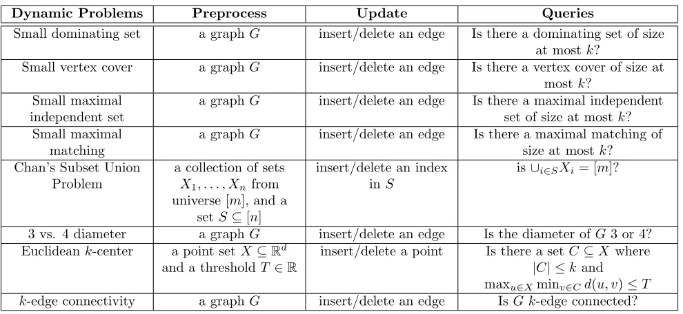
Table 4: Problems in PHdy that are not known to be inNPdy. The parameterk in every problem must be at most polylog(n) wherenis the size of the instance.

2. If the proof-sequence (π1, . . . , πk) is reward-maximizing (defined below), then we have xt = 1 for each t∈ {0, . . . , k} withDn(It) = 1,

The proof-sequence (π1, . . . , πk) is reward-maximizing iff the following holds. At each step t ≥ 1, given the past history (I0, . . . , It)and(π1, . . . , πt−1), the proof πt is chosen in such a way that maximizes the value ofyt. We say that such a proof πt isreward-maximizing.

Just as in the static setting, we can easily prove that Pdy _⊆NPdy _{and we conjecture thatP}dy _6=NPdy_. The big question left open in this paper is to resolve this conjecture.

Corollary 5.1. We havePdy⊆NPdy.

5.2 A complete problem inNPdy One of the main results in this paper shows that a natural problem called dynamic narrow DNF evaluation (denoted by DNFdy) is NPdy-complete. Intuitively, this means that (a) DNFdy ∈ NPdy, and (b) if DNFdy ∈ Pdy _then Pdy _{= NP}dy

.9 _{We now give an informal description}

of this problem.

Dynamic narrow DNF evaluation (DNFdy): An instance I of this problem consists of a triple (Z,C, φ), where Z = {z1, . . . , zN} is a set of N variables, C =

{C1, . . . , CM} is a set ofM DNF clauses, and φ:Z →

9_{To be more precise, condition (b) means that every problem} inPdy isPdy-reducible to DNFdy.

{0,1} is an assignment of values to the variables. Each clauseCjis a conjunction (AND) of at most polylog(N) literals, where each literal is of the form zi or ¬zi for some variablezi∈ Z. This is an YES instance if at least one clause C ∈ C is true under the assignment φ, and this is a NO instance if every clause in C is false under the assignment φ. Finally, an instance-update changes the assignment φ by flipping the value of exactly one variable inZ.

It is easy to see that the above problem is inNPdy. Specifically, if the current instance is an YES instance, then a proofπtsimply points to a specific clauseCj ∈ C that is true under the current assignmentφ. The proof

πt can be encoded using O(logM) bits. Furthermore, since each clause contains at most polylog(N) literals, the verifier can check that the clause Cj specified by the proof πt is true under the assignment φ in

O(polylog(N)) time. On the other hand, no proof can fool the verifier if the current instance is a NO instance (where every clause is false). All these observations can be formalized in a manner consistent with Definition5.3. We will prove the following theorem.

Theorem 5.1. The DNFdy problem described above is

NPdy-complete.

In order to prove Theorem 5.1, we consider an intermediate dynamic problem called First-DNFdy.

φ denote exactly the same objects as in the DNFdy problem described above. In addition, the symbol ≺

denotes a total order on the set of clausesC. The answer to this instance I is defined as follows. If every clause in C is false under the current assignment φ, then the answer toIis 0. Otherwise, the answer to Iis thefirst clauseCj ∈ Caccording to the total order≺that is true under φ. It follows that First-DNFdy is not a decision problem. Finally, as before, an instance-update for the First-DNFdy changes the assignment φby flipping the value of exactly one variable inZ.

We prove Theorem5.1as follows. (1) We first show that First-DNFdy is NPdy-hard. Specifically, if there is an algorithm for First-DNFdy with polylog update time and polynomial space complexity, then Pdy ₌ NPdy. We explain this in more details in Section5.2.1. (2) Using a standard binary-search trick, we show that there exists an O(polylog(n)) timereductionfrom First-DNFdy to DNFdy. Specifically, this means that if DNFdy ∈ Pdy_{, then we can use an algorithm for} DNFdy as a subroutine to design an algorithm for First-DNFdy with polylog update time and polynomial space complexity. Theorem5.1follows from (1) and (2), and the observation that DNFdy ∈NPdy.

5.2.1 NPdy-hardness of First-DNFdy Consider any dynamic decision problemDn∈NPdy. Thus, there exists a verifierVnforDnwith the properties mentioned in Definition5.3. Throughout Section5.2.1, we assume that there is an algorithm for First-DNFdywith polyno-mial space complexity and polylog update time. Under this assumption, we will show that there exists an algo-rithm An forDn that also has O(poly(n)) space com-plexity andO(polylog(n)) update time. This will imply theNPdy-hardness of First-DNFdy.

The high-level strategy: The algorithmAn will use the following twosubroutines: (1) The verifierVnforDn as specified in Definition5.2and Definition5.3, and (2) A dynamic algorithm A∗ that solves the First-DNFdy problem with polylog update time and polynomial space complexity.

To be more specific, consider any instance-sequence (I0, . . . , Ik) for the problem Dn. At step t = 0, after receiving the starting instance I0, the algorithm

An calls the subroutine Vn with the same input I0. The subroutine Vn returns an ordered pair (x0, y0). At this point, the algorithm An outputs the bit x0. Subsequently, at each step t ≥ 1, the algorithm An receives the instance-update (It−1, It) as input. It then calls the subroutineA∗_{in such a manner which ensures}

that A∗ _{returns a reward-maximizing proof π}

t for the verifierVn(see Definition5.3). This is explained in more

details below. The algorithmAn then calls the verifier

Vnwith the input ((It−1, It), πt), and the verifier returns an ordered pair (xt, yt). At this point, the algorithmAn outputs the bitxt.

To summarize, the algorithm An uses A∗ as a dynamic subroutine to construct a reward-maximizing proof-sequence (π1, . . . , πk) – one step at a time. Fur-thermore, after each step t≥1, the algorithmAn calls the verifier Vn with the input ((It−1, It), πt). The ver-ifier Vn returns (xt, yt), and the algorithmAn outputs

xt. Item (1) in Definition 5.3 implies that the algo-rithm An outputs 0 on all the NO instances (where

Dn(It) = 0). Since the proof-sequence (π1, . . . , πk) is reward-maximizing, item (2) in Definition 5.3 implies that the algorithm An outputs 1 on all the YES in-stances (where Dn(It) = 1). So the algorithm An al-ways outputs the correct answer and solves the problem

Dn. We now explain how the algorithm An calls the subroutine A∗_{, and then analyze the space complexity}

and update time ofAn. The key observation is that we can represent the verifier Vn as a collection of decision trees, and each root-to-leaf path in each of these trees can be modeled as a DNF clause.

The decision trees that define the verifier Vn: Let memVn denote the memory of the verifier Vn. We assume that during each stept≥1, the instance-update (It−1, It) is written in a designated region mem

(0)

Vn ⊆

memVn of the memory, and the proof πt is written in another designated region mem(1)_V

n ⊆ memVn of the memory. Each bit in memVn can be thought of as a boolean variable z ∈ {0,1}. We view the region

memVn\mem (1)

Vn as a collection of boolean variablesZ =

{z1, . . . , zN} and the contents of memVn\mem (1)

Vn as an assignment φ :Z → {0,1}. For example, if φ(zj) = 1 for some zj ∈ Z, then it means that the bit zj in

memVn \ mem (1)

Vn is currently set to 1. Upon receiving an input ((It−1, It), πt), the verifier Vn makes some probes inmemVn\mem

(1)

Vn according to some pre-defined procedure, and then outputs an answer (xt, yt). This procedure can be modeled as a decision tree Tπt. Each internal node (including the root) in this decision tree is either a ”read” node or a ”write” node. Each read-node has two children and is labelled with a variable

• Suppose that it is currently at a read-node of Tπt labelled withz ∈ Z. If φ(z) = 0 (resp. φ(z) = 1), then it goes to the left (resp. right) child of the node. On the other hand, suppose that it is currently at a write-node of Tπt which is labelled with (z, λ). Then it writesλ in the memory-bit z

(by setting φ(z) = λ) and then moves on to the only child of this node.

Finally, when it reaches a leaf-node, the verifier Vn outputs the corresponding label (x, y). This is the way the verifier operates when it is called with an input ((It−1, It), πt). The depth of the decision tree (the maximum length of any root-to-leaf path) is at most polylog(n), since as per Definition5.2the verifier makes at most polylog(n) many bit-probes in the memory while handling any input.

Each possible proofπfor the verifier can be specified using polylog(n) bits. Hence, we get a collection of

O(2polylog(n)_{) many decision treesT ={T}

π}– one tree

Tπ for each possible inputπ. This collection of decision treesT completely characterizes the verifierVn.

DNF clauses corresponding to a decision tree Tπt: Suppose that the proofπ is given as part of the input to the verifier during some update step. Consider any root-to-leaf path P in a decision treeTπ. We can naturally associate a DNF clause CP corresponding to this path P. To be more specific, suppose that the path P traverses a read-node labelled with z ∈ Z

and then goes to its left (resp. right) child. Then we have a literal ¬z (resp. z) in the clause CP that corresponds to this read-node.10 _{The clause C}

P is the conjunction (AND) of these literals, and CP is true iff the verifier Vn traverses the path P when π is the proof given to it as part of the input. Let C ={CP :

P is a root-to-leaf path in some treeTπ ∈ T } be the collection of all these DNF clauses.

Defining a total order ≺ over C: We now define a total order ≺ over C which satisfies the following property: Consider any two root-to-leaf paths P and

P0 _{in the collection of decision treesT. Let (x, y) and}

(x0, y0) respectively denote the labels associated with the leaf nodes of the paths P and P0. If CP ≺CP0, then y ≥ y0. Thus, the paths with higher y values appear earlier in≺.

Finding a reward-maximizing proof: Suppose that (I0, . . . , It−1) is the instance-sequence ofDnreceived by

An till now. By induction, suppose thatAn has man-aged to construct a reward-maximizing proof-sequence (π1, . . . , πt−1) till this point, and has fed this as input to

10_{W.l.o.g. we can assume that no two read nodes on the same} path are labelled with the same variable.

the verifier Vn (which is used as a subroutine). At the present moment, suppose thatAn receives an instance-update (It−1, It) as input. Our goal now is to find a reward-maximizing proofπtat the current stept.

Consider the tuple (Z,C, φ,≺) where

Z = memVn\mem (1)

Vn is the set of variables, C ={CP : P is a root-to-leaf path in some decision treeTπ} is the set of DNF clauses, the assignment φ:Z → {0,1}

reflects the current contents of the memory-bits in

memVn \ mem (1)

Vn, and ≺ is the total ordering over C described above. Let CP0 ∈ C be the answer to this

First-DNFdy instance (Z,C, φ,≺), and suppose that the path P0 belongs to the decision treeTπ0 corresponding

to the proof π0. A moment’s thought will reveal that

πt=π0 is the desired reward-maximizing proof at step

t we were looking for, because of the following reason. Let (x0, y0) be the label associated with the leaf-node in P0. By definition, if the verifier gets the ordered pair ((It−1, It), π0) as input at this point, then it will traverse the pathP0 in the decision treeTπ0 and return

the ordered pair (x0, y0). Furthermore, the path P0

comes first according to the total ordering ≺, among all the paths that can be traversed by the verifier at this point. Hence, the path P0 _{is chosen in such a way}

that maximizes y0_{, and accordingly, we conclude that}

yt=y0 is a reward-maximizing proof at stept.

Wrapping up: Handling an instance-update (It−1, It). To summarize, when the algorithm An re-ceives an instance-update (It−1, It), it works as follows. It first writes down in the instance-update (It−1, It) in mem(0)_Vn and accordingly updates the assignment φ :

Z → {0,1}. It then calls the subroutine A∗ on the First-DNFdy instance (Z,C, φ,≺). The subroutine A∗

returns a reward-maximizing proof πt. The algorithm

Anthen calls the verifierVnas a subroutine with the or-dered pair ((It−1, It), πt) as input. The verifier updates at most polylog(n) many bits inmemVn and returns an ordered pair (xt, yt). The algorithm An now updates the assignment φ:Z → {0,1} to ensure that it is syn-chronized with the current contents ofmemVn. This re-quires O(polylog(n)) many calls to the subroutine A∗

for the First-DNFdy instance. Finally, An outputs the bit xt∈ {0,1}.

Bounding the update time ofAn: Notice that after each instance-update (It−1, It), the algorithmAnmakes one call to the verifierVn and at most polylog(n) many calls to A∗_{. By Definition 5.2, the call to V}

n requires

O(polylog(n)) time. Furthermore, we have assumed that A∗ _{has polylog update time. Hence, each call to}