Original citation:
Drovandi, Christopher C., Moores, Matthew T. and Boys, Richard J.. (2018) Accelerating pseudo-marginal MCMC using Gaussian processes. Computational Statistics & Data Analysis, 118.
Permanent WRAP URL:
http://wrap.warwick.ac.uk/92705
Copyright and reuse:
The Warwick Research Archive Portal (WRAP) makes this work of researchers of the University of Warwick available open access under the following conditions.
This article is made available under the Creative Commons Attribution 4.0 International license (CC BY 4.0) and may be reused according to the conditions of the license. For more
details see: http://creativecommons.org/licenses/by/4.0/
A note on versions:
The version presented in WRAP is the published version, or, version of record, and may be cited as it appears here.
Accelerating Pseudo-Marginal MCMC using Gaussian Processes
C. C. Drovandi*, M. T. Moores† and R. J. Boys‡
*Australian Centre of Excellence for Mathematical and Statistical Frontiers and Queensland University of Technology, Brisbane, Australia 4001
† University of Warwick, Coventry CV4 7AL, United Kingdom ‡ Newcastle University, Newcastle upon Tyne NE1 7RU, United Kingdom
email: [email protected]
October 3, 2017
Abstract
The grouped independence Metropolis-Hastings (GIMH) and Markov chain within Metropolis (MCWM) algorithms are pseudo-marginal methods used to perform Bayesian inference in la-tent variable models. These methods replace intractable likelihood calculations with unbiased estimates within Markov chain Monte Carlo algorithms. The GIMH method has the posterior of interest as its limiting distribution, but suffers from poor mixing if it is too computation-ally intensive to obtain high-precision likelihood estimates. The MCWM algorithm has better mixing properties, but tends to give conservative approximations of the posterior and is still expensive. A new method is developed to accelerate the GIMH method by using a Gaussian process (GP) approximation to the log-likelihood and train this GP using a short pilot run of the MCWM algorithm. This new method called GP-GIMH is illustrated on simulated data from a stochastic volatility and a gene network model. The new approach produces reasonable posterior approximations in these examples with at least an order of magnitude improvement in computing time. Code to implement the method for the gene network example can be found athttp://www.runmycode.org/companion/view/2663.
Keywords: Gaussian processes, likelihood-free methods, Markov processes, particle Markov
1
Introduction
Bayesian inference for high-dimensional latent variable models is currently challenging. In particular Markov chain Monte Carlo (MCMC) samplers can suffer from poor mixing due to correlation between the parameter of interest and the latent variables. Beaumont (2003) and Andrieu and Roberts (2009) have introduced pseudo-marginal methods to improve the statistical efficiency of MCMC. These methods work by replacing the actual likelihood with an unbiased likelihood estimate in the Metropolis-Hastings ratio. This allows proposals for the Markov chain to be made directly on the space of the parameter of interest, rather than conditional on the value of a set of the latent variables.
One of these methods, the grouped independence Metropolis-Hastings (GIMH) method by Beaumont (2003), recycles the likelihood estimate for the current value of the chain to the next iteration. Andrieu and Roberts (2009) have shown that the GIMH method has the desired posterior as its limiting distribution, which is why it has received considerable attention in the literature (Andrieu et al. (2010); Doucet et al. (2015)). However, a drawback of the GIMH method is that it can suffer from poor mixing if it is too computationally expensive to estimate the likelihood with high precision.
The other method, the Markov chain within Metropolis (MCWM, Beaumont (2003)) algo-rithm, estimates the likelihood at both the current and proposed values of the Markov chain at every iteration. This method generally possesses better mixing properties as it is able to escape an overestimated likelihood value by re-estimating it at the next MCMC iteration. However, the MCWM method does not have the posterior distribution of the parameter of interest as its limiting distribution. Because of this, MCWM has received comparatively less attention.
In this paper we make use of a Gaussian process (GP) to accelerate the GIMH method while at the same time accepting some approximation to the posterior distribution.
Wilkinson (2014) proposes that GPs be used to accelerate approximate Bayesian computation (ABC) methods where the likelihood is approximated by generating many model simulations from each proposed parameter value, and measuring the distance between observed and sim-ulated data through a careful choice of summary statistics. Here GPs are used to emulate the actual (ABC) log-likelihood surface based on noisy estimates obtained through simulation. The method iteratively uses the GP to discard implausible parts of the parameter space, re-trains the GP in the updated not-implausible part of the parameter space and continues this process until the GP fit has been deemed as satisfactory. The final GP is then used within an MCMC method to predict the log-likelihood surface at all proposed values of the parameter of interest. GPs have also been used for ABC by Meeds and Welling (2014), Gutmann and Corander (2016) and J¨arvenp¨a¨a et al. (2016).
Our experience with MCWM is that it is generally conservative (inflated posterior variance), allowing the tails of the posterior to be explored. The fitted GP is used instead of expensive likelihood estimates within the GIMH method. We introduce further novelties into our method to make it practically useful.
The paper has the following outline. In Sections 2.1 and 2.2 we provide a brief overview of pseudo-marginal methods and GPs, respectively. In Section 2.3 we present our new method, GP-GIMH, which uses the MCWM algorithm to train the GP and subsequently uses the GP to accelerate the GIMH method. Finally, in Section 4, we conclude with a discussion.
2
Accelerated Pseudo-Marginal MCMC
In this section we give some background on pseudo-marginal MCMC methods and Gaussian processes before describing how, by emulating the log-likelihood using a GP, we can accelerate pseudo-marginal MCMC.
2.1 Pseudo-Marginal MCMC
Suppose we have observed datayinYwhich is described by a statistical model with likelihood function p(y|θ) and depends on an unknown parameter θ in Rd. Prior beliefs about the
parameter are summarised by the prior densityp(θ). We assume that the model requires, or is facilitated by, an auxiliary variablexinX, whose value is not of direct interest. In this scenario the complete data likelihood is p(y,x|θ) = p(y|x,θ)p(x|θ) and leads to the observed data likelihood p(y|θ) = R
Xp(y|x,θ)p(x|θ)dx. Ideally this observed data likelihood is combined with the prior to make inferences about the parameters via the posterior density p(θ|y) ∝ p(y|θ)p(θ). However, in non-toy problems the observed data likelihood is an analytically intractable integral. Therefore the parameter posterior is accessed as the marginal of the joint posterior for all unknowns, that is, viap(θ|y) =R
Xp(θ,x|y)dx.
A standard Bayesian approach for fitting such a latent variable model is to develop an MCMC algorithm that samples the joint posteriorp(θ,x|y) and marginalises by ignoring the x sam-ples. A common approach is to develop an MCMC algorithm using two blocks,θ andx, that iteratively samples from the full conditionals p(θ|x,y) and p(x|θ,y). A key problem with such algorithms is that they can mix poorly because of high posterior correlation between the blocksθ and x. Further, for non-trivial state space models,p(x|θ,y) cannot be sampled directly and is difficult to sample efficiently (see Andrieu et al. (2010) for a discussion). In an attempt to overcome the mixing issue, Beaumont (2003) develop algorithms that replace the computationally intractable likelihoodp(y|θ) with an unbiased estimate ˆp(y|θ). The un-derpinning mathematics of these pseudo-marginal MCMC algorithms is studied in Andrieu and Roberts (2009) and they develop conditions under which they indeed have the correct posterior distributionp(θ|y) as their limiting distribution. A simple example of an unbiased likelihood estimate is one obtained through importance sampling, namely
ˆ
p(y|θ) = 1
N
N
X
i=1
p(y|xi,θ)p(xi|θ)
g(xi)
wherex1, . . . ,xN
iid
∼g(x) andgis an importance density defined onX. Alternative approaches to obtaining an unbiased likelihood estimate are available. For example, Andrieu et al. (2010) show that when the model of interest is a state-space model, the likelihood p(y|θ) can be estimated unbiasedly using a particle filter withN particles. Such pseudo-marginal methods are referred to as particle Markov chain Monte Carlo (PMCMC). We consider models in the state-space form in Section 3 and use the bootstrap particle filter of Gordon et al. (1993) to obtain an unbiased likelihood estimator.
B´erard et al. (2014) establish a log-normal central limit theorem for the particle filter. In PMCMC, the likelihood is estimated with multiplicative noise, ˆp(y|θ) =W p(y|θ),where the random weightW is strictly positive withE[W] = 1. The CLT defines a limiting distribution
for the noise in which logW −→ N −d ασ2/2, ασ2
as the dimension (of the state space X)
T → ∞. Here σ2 is the asymptotic variance of the estimator, andα is the asymptotic ratio ofT toN as bothT, N → ∞, and is usually taken to be 1. Doucet et al. (2015) observe that this limiting distribution is a good fit for the noise, even for modest values ofT andN. The log-normal CLT is very useful for theoretical analysis of PMCMC algorithms as shown, for example, by Doucet et al. (2015) and Medina-Aguayo et al. (2016). We assume log-normality of ˆp(y|θ) in our GP model.
The first algorithm developed by Beaumont (2003), known as grouped independence Metropolis-Hastings (GIMH), is shown in Appendix A. This is essentially a standard Metropolis-Metropolis-Hastings algorithm in which the intractable likelihood at a new proposalθ∗ is replaced by an unbiased likelihood estimate. Note that the likelihood at the current valueθ is not re-estimated but simply recycled from the previous iteration.
Andrieu and Roberts (2009) show that the GIMH algorithm has the posterior p(θ|y) as its limiting distribution. If we denote all the random numbers (assumed to be uniformly distributed without loss of generality) used to produce an unbiased likelihood estimate as η ∈ [0,1]s and considering a target posterior distribution on the extended space of (θ,η), the θ marginal target of interest is proportional to p(θ)E[ˆp(y|θ,η)] where ˆp(y|θ,η) is the likelihood estimate given the random numbers and the expectation is taken with respect to the distribution ofηgivenθ. The unbiased nature of the likelihood estimator implies that the expectation isp(y|θ) giving the desired posterior distribution as the target. This theoretically appealing property has led to the GIMH method becoming more prominent in the literature (e.g. Andrieu et al. (2010), Doucet et al. (2015) and Sherlock et al. (2017)) compared to the other approach of Beaumont (2003), the Monte Carlo within Metropolis (MCWM) algorithm. However, the GIMH method can get stuck when the likelihood is substantially overestimated at any given iteration. Doucet et al. (2015) suggest that for good performance in the GIMH algorithm, the log-likelihood should be estimated with a standard deviation between 1.0 and 1.7. However, in complex applications, it may be computationally difficult to achieve this goal.
for the geometric ergodicity and hence the existence of an invariant distribution of MCWM for large enough N. The conditions are that the idealised chain (the chain that uses exact likelihood evaluations) is geometrically ergodic, the weightsW are uniformly integrable and the weights satisfy uniform exponential bounds on their densities close to 0. These conditions are quite weak when the parameter space is compact. In our experience, MCWM generally produces an approximate posterior that is less precise than the actual posterior for finiteN, and thus could be considered a conservative method in the sense that the posterior variances are overestimated.
Our aim is to accelerate the GIMH method by emulating the (unobserved) true log-likelihood surface as a function ofθwith a GP, where the GP is trained in relevant parts of the parameter space based on the output of a short run of MCWM.
2.2 Gaussian Processes
Gaussian processes can be used as a prior distribution to describe uncertainty about an unknown function f(·). They are characterised by a mean function mβ(θ) and covariance function Cγ(θ,θ0) = cov{f(θ), f(θ0)}, where β and γ are so-called hyperparameters of the GP. A Gaussian process has the property that the joint distribution for the values of the function at a finite collection of points has a multivariate normal distribution; see, for example, Rasmussen and Williams (2006). In this paper, the function we wish to emulate is the log-likelihood function f(θ) = logp(y|θ). We assume a GP prior with mean function mβ(θ) =
β0+Ppk=1βkθk+Ppk=1βk+pθk2,whereθk is thekth component of the parameter vectorθand β= (β0, β1, . . . , β2p)>. We also assume that the log-likelihood surface is smooth and so take a squared exponential covariance function
Cγ(θ,θ0) =δcexp
(
−1
2 p
X
k=1
(θk−θk0)2
r2
k
)
,
with hyper-parameters γ= (δc, r1, . . . , rp)>.
Only noisy estimates of the likelihood are available and so we need to model their sampling distribution. We rely on the log-normal CLT (B´erard et al., 2014) and assume multiplicative noise with varianceδ. This assumption is not quite correct as the estimates are not exactly log-normal for finiteN, even when drawn from a particle filter. Additionally, there may be some dependence of their accuracy on the parameter valueθ. Nevertheless we believe that this description captures the key aspects of the sampling distribution and has the great benefit of simplifying the form of GP prediction. Specifically, taking account of the variability in the function evaluations requires that we add a nugget term to the covariance function, so that cov{fˆ(θ),fˆ(θ0)} = Cγ(θ,θ0) +δ1(θ = θ0), where 1(·) denotes the indicator function, which is 1 if its argument is true and 0 otherwise. We can estimate the GP hyperparameter ξ= (β,γ, δ) using a training sample containing evaluations of the log-likelihood estimates at a set ofJ (input) values Θ. We denote this training sample by DT ={θj,fˆ(θj)}Jj=1.
identity matrix. This result is obtained by integrating over the random variables describing the actual function values at the training input values and is thus often referred to as the marginal likelihood. The hyperparameter can therefore be estimated via maximising the log marginal likelihood, that is, taking
ˆ
ξ= arg min ξ
{f(Θ)−mβ(Θ)}>{Cγ(Θ,Θ) +δI}−1{f(Θ)−mβ(Θ)}+ log|Cγ(Θ,Θ) +δI|
.
(1)
In practice the estimate is obtained using a numerical scheme and so we use multiple starting values for the optimisation process in order to obtain a result that we believe to be close to the maximum marginal likelihood estimate.
The fitted GP is the posterior distribution of the log-likelihood function in light of the observed training data. It can be used to predict the value of the log-likelihood functionf(θ) at any valueθ as its posterior distribution isf(θ)|DT ∼ N {m∗(θ), s∗(θ)2}, where
m∗(θ) =mβˆ(θ) +Cγˆ(Θ,θ)>{Cγˆ(Θ,Θ) + ˆδI}−1{f(Θ)−mβˆ(Θ)}, (2)
s∗(θ)2=Cγˆ(θ,θ)−Cγˆ(Θ,θ)>{Cγˆ(Θ,Θ) + ˆδI}−1Cγˆ(Θ,θ), (3)
and Cγˆ(Θ,θ) is a J ×1 vector, with Cγˆ(Θ,θ)j = Cγˆ(θj,θ). Note that the computational complexity of the GP prediction isO(J3). If the hyperparameter estimate ˆξ and the training dataDT are static then the inverse computation {Cγˆ(Θ,Θ) + ˆδI}−1 can be re-used for each
new θ. However, if additional training data is added then the inverse must be re-computed. In such cases it is of interest to limit the number of training pointsJ.
2.3 Pseudo-Marginal MCMC using Gaussian Processes
This section describes how to deploy a GP to accelerate the GIMH algorithm. The new algorithm, called GP-GIMH, is given in Algorithm 1. More detail about each of the steps is given below.
As described in the previous section, we use a pilot run of the MCWM algorithm to gen-erate the design points Θ, during which we record the parameter value and both estimated log-likelihood values encountered during the MCWM algorithm (even those from rejected proposals) in the training sample. Our motivation for using MCWM to determine the train-ing sample for the GP is three-fold: (i) it harnesses the observed data and thus most of the training points will be parameter values with non-negligible posterior density; (ii) it has good mixing properties ensuring that the GP is trained at a wide range of plausibleθ values; and (iii) the MCWM method is conservative and so it can provide good coverage of the tails of the posterior distribution. However, since MCWM is conservative, it may visit parameter regions where the log-posterior is very low (especially for proposals rejected by the algorithm) and so we suggest removing points with very low log-posterior (ignoring the normalising constant independent ofθ) values from the training sample so that the training of the GP focuses on plausible regions of the parameter space.
that samples from the following approximate posterior
pGP(θ|y)∝exp
m∗(θ) +s ∗(θ)2
2
p(θ),
where the exponential term is the mean of the log-normal distribution implied by the GP assumption. A standard MCMC algorithm could be applied to sample frompGP(θ|y). How-ever, for pGP(θ|y) to be a reasonable approximation of p(θ|y) we require s∗(θ) to not be
too large across important parts of the parameter space. When s∗(θ) is too large at a pro-posed value θ∗, i.e.s∗(θ∗) > for some chosen threshold , we apply an intervention. Also, to reduce computation, we would like to limit the number of times where interventions are necessary. To achieve this, we adopt a GIMH-style algorithm. Instead of evaluating the mean of the log-normal density directly, we simulate a log-likelihood estimate from the fitted GP, N {m∗(θ∗), s∗(θ∗)2}. When s∗(θ∗) > and θ∗ is accepted, there is an increased risk of obtaining a sticky period at θ∗. If s∗(θ∗) > and θ∗ is rejected we do not apply an inter-vention. The intervention involves obtaining a more accurate GP prediction to check if θ∗ was wrongly accepted or to help reduce sticky periods. We obtainK independent estimates of f(θ∗) = logp(y|θ∗) using the same method (e.g. importance sampling or particle filter estimates) as in the training phase and determine their mean. Under the log-normal CLT, this mean also has a normal distribution: ¯fK(θ∗)∼ N {f(θ∗),ˆδ/K}where ˆδ is the maximum likelihood estimate of δ found in (1). We can incorporate this information into our beliefs about the log-likelihood at this point using a simple Bayes update, to give
f(θ∗)|DT,f¯K(θ∗)∼ N
m∗(θ∗)/s∗(θ∗)2+Kf¯K(θ∗)/δˆ 1/s∗(θ∗)2+K/δˆ .
1
1/s∗(θ∗)2+K/δˆ
!
, (4)
Therefore the total number of independent log-likelihood estimates needed to secure a suffi-ciently accurate GP prediction is roughlyK=dδˆ{−2−s∗(θ∗)−2}e. If these multiple estimates can be farmed out across sayAavailable processors then the number of estimates in each batch to achieve this goal isdK/Ae.
We allow a burn-in phase consisting ofB iterations where such additional likelihood estimates can be appended to the training sampleDT. The motivation for this burn-in phase is to assist the GP in being trained in important regions not explored sufficiently in the MCWM phase. We find in Section 3 that the burn-in phase is useful in applications where it is very expensive to estimate the likelihood. The computational drawback of the burn-in phase is that the matrix inversion in (2) and (3) must be re-computed. However, in demanding applications these additional matrix inversions can be relatively cheap. It would be feasible to re-estimate the GP hyperparameter after the burn-in phase if desired. We note that the relative computing time for this should be short in complex applications as the current hyperparameter estimate can be used as a starting value.
perform another Metropolis-Hastings accept/reject step but where the log-likelihood estimate is simulated based on (4).
The value ofcontrols the level of uncertainty allowed in the GP prediction when parameter values are accepted. If is set too large then a parameter value may be accepted with a grossly overestimated log-likelihood value and lead to stickiness in the Markov chain, similar behaviour that can be observed in the standard GIMH method. Smaller values ofwill lead to runs that are generally less sticky, but more computation is required to satisfy the constraint
s∗(θ∗)< . Recall that Doucet et al. (2015) suggest that the log-likelihood should be estimated with a standard deviation of roughly 1 for the GIMH method to have similar statistical efficiency to a standard Metropolis-Hastings method where the likelihood is available. For our examples we find that <2 is a suitable choice.
In practice we choose by performing some very short pilot runs and ensuring that for the majority of acceptedθ∗ we have s∗(θ∗)< . Some insight into a suitable value of may also be obtained by inspecting the empirical distribution of the GP prediction standard deviations at the training points{s∗(θj), θj ∈ DT}. Ifis not in the upper tail of this distribution then this indicates that the GP training set DT requires additional training points as otherwise many additional log-likelihood estimates will be needed in GP-GIMH and little algorithmic speed-up will be obtained.
The speed-up of the GP-GIMH approach is roughlyF/(2ρF+G) whereF is the time taken to run GIMH forQ iterations, 2ρF is the time forLiterations of the MCWM pre-computation step where ρ= L/Q and the value of 2 denotes the fact that two likelihood estimations are required at each iteration of MCWM, andGis the remaining time of the GP-GIMH method. In this paper we assume that F is very large; it is computationally demanding to estimate the likelihood. In such casesGmay be negligible in comparison, in which case the speed-up is roughlyQ/(2L). Thus it is of interest to setL small. However, ifL is set too small thenG
may become non-negligible since the GP may be too uncertain across much of the parameter space. Furthermore we note thatLwill naturally need to increase as the parameter dimension grows (although it may be of interest to increaseQ as well). The value of G will also likely increase with the parameter dimension since it becomes increasingly difficult to train the GP in areas of non-negligible posterior support. In summary, the GP-GIMH approach does suffer from the curse of dimensionality. Nonetheless, in Section 3, we demonstrate that it is possible to achieve significant speed-ups on non-trivial models of moderate dimension. It is important to note that the above discussion only considers the computational gains. We generally find also with GP-GIMH that sticky periods can be mitigated, adding to the overall efficiency gains of GP-GIMH.
Our approach uses the MCWM algorithm to train the GP whereas Wilkinson (2014) uses a history matching approach, which iteratively fits a GP to samples drawn from a hypercube, which shrinks upon each successive GP fit. This process may be expensive in moderate dimensions if uninformative priors are used and it does not exploit the correlation between parameters as our approach does. We compare the two training approaches on one of the examples later. Our remaining MCMC algorithm that uses GP predictions is similar to Wilkinson (2014). However, we include the novel aspects of obtaining additional likelihood estimates when required and a burn-in phase.
Algorithm 1GP-GIMH algorithm.
Input: threshold, burn-in B and the number of MCMC iterations (iters)
Output: MCMC output θ1, . . . ,θiters
1: Perform an MCWM algorithm forLiterations to help determine an initial training sample. See the text for more details. The training sample after these processes is denoted as
DT ={θj,fˆ(θj)}Jj=1
2: Estimate the hyperparameter ξ= (β,γ, δ) of a GP using the training sampleDT
3: Simulate φ0 ∼ LN {m∗(θ0), s∗(θ0)2} from the GP with hyperparameter ˆξ. θ0 can be chosen based on the MCWM pilot run
4: for i= 1 toitersdo
5: Proposeθ∗ ∼q(·|θi−1)
6: Simulateφ∗ ∼ LN {m∗(θ∗), s∗(θ∗)2} from the GP with hyperparameter ˆξ
7: Compute α= minn1, φ∗p(θ∗)q(θi−1|θ∗)
φi−1p(θi−1)q(θ∗|θi−1)
o
8: Draw u∼ U(0,1)
9: if u < αthen
10: if s∗(θ∗)≤ then
11: Set φi =φ∗ andθi =θ∗
12: else
13: Obtain A batches of dK/Ae independent likelihood estimates and update m∗(θ∗) and s∗(θ∗) using (4)
14: If i≤B then append the likelihood estimates to the training sampleDT.
15: Simulate φ∗ ∼ LN {m∗(θ∗), s∗(θ∗)2}from the GP with hyperparameter ˆξ
16: Compute α= min
n
1,φi−φ1∗pp((θθ∗i−)q1()θqi(−θ∗1|θ|θ∗i−)1)
o
17: if u < αthen
18: Setφi=φ∗ and θi =θ∗
19: else
20: Setφi=φi−1 and θi=θi−1
21: end if
22: end if
23: else
24: Setφi =φi−1 and θi =θi−1
25: end if
26: end for
2.4 Related Literature
GPs have been used for the emulation of complex deterministic models by Kennedy and O’Hagan (2000, 2001) and for complex stochastic models by Henderson et al. (2009, 2010) and Baggaley et al. (2012). Conrad et al. (2016) use local polynomials or GPs in a Metropolis-Hastings algorithm to reduce the number of model evaluations that are required. However, the focus of Conrad et al. (2016) is not on applications where a stochastic likelihood estimator is available.
Tran et al. (2017) develop a variational Bayes approach that can be used in any applica-tion where an unbiased likelihood estimator is available to approximate the posterior more efficiently compared to GIMH. However, the variational approximation is typically of a para-metric form and assumptions are sometimes made that the parameters are independent a posteriori.
Rasmussen (2003) use GPs to accelerate the Hamiltonian Monte Carlo (HMC) method for Bayesian inference when posterior density evaluation is expensive. The proposal distribution in HMC involves (approximately) solving a Hamiltonian system, and requires several evalu-ations of the posterior distribution. The GP is trained from a pilot HMC run and used to approximate posterior evaluations required in the HMC proposal. This method remains exact as the GP is used only for the proposal and a Metropolis-Hastings (MH) correction is applied to account for the fact that the Hamiltonian is only solved approximately. The MH correction step requires an evaluation of the (expensive) exact posterior density.
A related literature is on the delayed-acceptance MCMC method (Christen and Fox, 2005). Here each proposed parameter goes through an initial Metropolis-Hastings step where the actual posterior density is replaced by a computationally cheap posterior approximation. The idea of the method is that ‘poor’ proposals can be rejected quickly and the majority of ‘promising’ proposals make it through to the next Metropolis-Hastings stage, which involves evaluations of the exact posterior density. The second Metropolis-Hastings step is constructed so that the Markov chain has the correct limiting distribution. As an example, Golightly et al. (2015) perform Bayesian inference for Markov jump processes using the corresponding linear noise approximation in the screening Metropolis-Hastings step. Sherlock et al. (2017) consider a more general approach and use aknearest neighbour surrogate within a delayed-acceptance MCMC algorithm when the likelihood is expensive or when the likelihood is estimated unbi-asedly. Although the delayed-acceptance MCMC approach is exact, Golightly et al. (2015) and Sherlock et al. (2017) report efficiency gains of generally less than an order of magnitude. Our motivation here is to obtain a significant speed-up in very complex applications whilst accepting some approximation to the posterior.
3
Examples
0 1000 2000 3000 4000 5000 −4
−2 0 2 4
t
y
Figure 1: Data simulated from the stochastic volatility model of Section 3.1.1.
3.1 Stochastic Volatility Example
3.1.1 Model and Data
We illustrate our method by analysing data simulated from a stochastic volatility model in Chopin et al. (2013); this paper (and some of the references therein) give more details of the model construction and its interpretation. The observation at time t is scalar and has distributionyt∼ N(µ+βvt, vt), wherevtdenotes the evolving and unobserved variance of the observation process. Hereµ and β are static parameters. The evolution of the state process followsλvt=zt−1−zt+Pkj=1fj,wherek∼ Po(λξ2/w2),c1:k
iid
∼ U(t−1, t),f1:k
iid
∼ Exp(ξ/w2), and zt = e−λzt−1+Pkj=1e−λ(t−cj)fj, and Po, U and Exp denote the Poisson, uniform and exponential distributions respectively. Here w2, ξ and λ are additional static parameters so that the full parameter set is θ = (w2, µ, ξ, β, λ). We assume our prior has independent components with w2, ξ ∼ Exp(5), µ, β ∼ N(0,2) and λ ∼ Exp(1). Also we initialise the z
-process usingz0 ∼ Ga(ξ2/w2, ξ/w2), that is, a gamma distribution with meanξ and standard
deviationw.
The observed data for this example has been generated from the model using the same pa-rameter values as in Chopin et al. (2013), namely w2 = 0.0625, µ = 0, ξ = 0.25, β = 0 and
λ= 0.01. However, our data are a longer series with 5000 observations (as opposed to their 1000 observations). The length of our time series creates a challenging problem for PMCMC algorithms. The data are shown in Figure 1.
3.1.2 Implementation Details
is compared to a close-to-optimal GIMH run. To further improve the performance of GIMH, we use the multiple-core PMCMC approach of Drovandi (2014) which uses multiple cores (here A= 16 cores) to obtain independent likelihood estimates for each proposed parameter value and takes the average in order to reduce the variance of the estimated likelihood. We run 100K iterations of GIMH. We also consider MCWM with N = 800 but only run it for 50K iterations as this algorithm requires two likelihood estimates at each iteration. We use the 16 cores in a similar way to improve the accuracy of MCWM. To use as a gold standard for comparison purposes, we run the GIMH algorithm for 400K iterations (withN = 800).
For the MCWM pre-computation step of GP-GIMH we use L = 1500, producing ≈ 3000 likelihood estimates. During this step, we adapt the covariance matrix of the multivariate normal random walk proposal every 10th iteration, following an initial 50 iterations. Recall that this MCWM output is only used to train the GP. We do not take advantage of any parallel computing in the MCWM pre-computation phase to illustrate that GP-GIMH can be effective even when the likelihood is not estimated as precisely as in our implementations of the standard GIMH and MCWM methods. The maximum log-posterior estimate encountered during the MCWM pre-computation phase is roughly −4610. We discard any log-posterior estimates below −4700. The main motivation for selecting this value is to eliminate two extreme log-likelihood estimates (-8926 and -6362) from the training. There are 18 other log-likelihood estimates that are also below this chosen threshold. To investigate the effect of the training sample size,J, we use all samples obtained from the MCWM pre-computing step and also thin the output by a factor of 2, producing (roughly)J = 1500 andJ = 3000. For comparison purposes the remaining part of GP-GIMH (again 100K iterations) uses the same multivariate normal random walk as GIMH/MCWM. No burn-in phase is used for GP-GIMH (i.e. no additional log-likelihood estimates are added to the training sample). We considervalues of 1, 1.5 and 2. When the tolerance condition is not met, we obtain dK/Ae
batches of A= 16 independent likelihood estimates. We also make the 16 cores available in the remaining part of the GP-GIMH algorithm as Matlab automatically parallelises some of the computations. We run the full GP-GIMH procedure independently five times for each combination ofJ and .
To simplify comparisons between methods, we assume that a suitable starting value and multi-variate normal random walk covariance matrix have already been determined, which are used for each algorithm (except the MCWM pre-computing phase, which adaptively determines a covariance matrix). Here we use the true parameter value to initialise the chain (unless otherwise stated) and an updating matrix obtained from some pilot runs. We note that, in reality, it is likely that the GP-GIMH algorithm would be faster at determining a suitable covariance matrix given that pilot runs can be performed quickly. This could also be a strong motivation for using a GP-GIMH algorithm if exact inferences are necessary (up to Monte Carlo error). We now explore the accuracy of the GP-GIMH algorithm in determining the posterior distribution.
3.1.3 Results
We find the marginal posterior estimates of GP-GIMH are insensitive to the choices of
Table 1: Upper triangular part of the posterior correlation matrix for θ obtained from the gold standard GIMH/GP-GIMH (first run with J ≈ 1500 and = 1.0) algorithms for the stochastic volatility model.
µ ξ β λ
w2 -0.91/-0.90 -0.03/0.00 -0.05/-0.02 0.03/0.01
µ 0.02/0.02 0.05/0.01 -0.03/0.00
ξ 0.63/0.68 -0.07/-0.06
β -0.40/-0.33
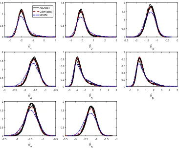
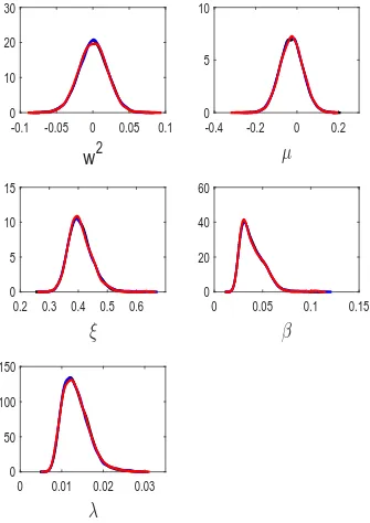
results for= 1. Shown in the figures are results from the 5 independent runs of GP-GIMH, as well as the results produced by GIMH (gold standard run) and MCWM. One possible metric to assess the accuracy of the results from the different approximations is the total variation (TV) distance between the posterior estimates (e.g. kernel density estimates from the posterior samples, see Appendix K for more details) obtained from an approximation and the gold standard run. It is important to note that even the GIMH run suffers from Monte Carlo variability. Tables 1 and 2 in Appendix C show the TV distances between the univariate and bivariate posteriors, respectively, for the results obtained from GIMH (N = 800), MCWM and GP-GIMH (results averaged over 5 runs) with respect to the gold standard GIMH run. Due to the computational expense of computing the TV over two dimensions we only consider GP-GIMH results for= 1.0 and J ≈3000. From the tables it is clear that, unsurprisingly, GIMH is the most accurate. However, GP-GIMH appears to be more accurate than MCWM, except for any marginal or bivariate posterior that involves the parameterλ. Figures 2 and 3 show a clear bias in the estimated posterior from GP-GIMH forλ. Further, it appears that the GP-GIMH algorithm has more difficulty approximating the posterior distributions that show some skewness.
One drawback of GP-GIMH is there is some between-run variability, which is more apparent for the posterior distributions that deviate away from symmetry. It is likely that this variabil-ity comes from different GP fits resulting from different MCWM pre-computing runs. From Figure 3 it appears that the between-run variability is reduced slightly when using the larger training sample size,J ≈3000. We attempt to validate this numerically. Here we consider the TV distances between the marginal densities produced from an individual run of GP-GIMH and the average marginal densities over the five runs of GP-GIMH. We then average these five distances to produce a single measure of the between-run variability. The table for different combinations ofand J are shown in Appendix C. It is indeed evident that the between-run variability is generally reduced for largerJ. Further, whenJ ≈1500, we see an increase in the between-run TV distances for the parametersξ,β and λwhen is increased to 2.0. This is due to the distortion in the tails of these posteriors that is occasionally present when= 2.0. When J ≈3000, we see an increase in the between-run TV forλwhen is increased for the same reason.
-0.08 -0.05 -0.02 0.01 0.04 0.07 0.1 w2 0 10 20 GP-GIMH GIMH (gold) MCWM
-0.3 -0.2 -0.1 0 0.1 0.2
µ 0 2 4 6 8
0.3 0.4 0.5 0.6
ξ
0 5 10
0 0.02 0.04 0.06 0.08 0.1
β 0 10 20 30 40 50
0 0.01 0.02 0.03
λ
0 50 100 150
Figure 2: Estimated marginal posterior densities for the stochastic volatility example from runs of the gold standard GIMH (red dash) and MCWM (blue dash-dot) algorithms and five independent runs of the GP-GIMH (black solid) algorithm withJ ≈1500 and= 1.
-0.08 -0.05 -0.02 0.01 0.04 0.07 0.1
w2 0 10 20 GP-GIMH GIMH (gold) MCWM
-0.3 -0.2 -0.1 0 0.1 0.2
µ 0 2 4 6 8
0.3 0.4 0.5 0.6
ξ
0 5 10
0 0.02 0.04 0.06 0.08 0.1
β 0 10 20 30 40 50
0 0.01 0.02 0.03
λ
0 50 100 150
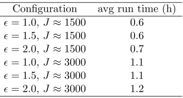
Table 2: Average run times for GP-GIMH (excluding the MCWM pre-computing phase and GP fitting) for different combinations ofJ and for the stochastic volatility example. The average time for GP training and fitting is 2.1 hours.
Configuration avg run time (h)
= 1.0, J ≈1500 0.6
= 1.5, J ≈1500 0.6
= 2.0, J ≈1500 0.7
= 1.0, J ≈3000 1.1
= 1.5, J ≈3000 1.1
= 2.0, J ≈3000 1.2
Table 2 shows the run times (averaged over the 5 independent runs) for GP-GIMH (excluding the MCWM pre-computing phase and GP fitting) for different combinations ofJ and. There is little sensitivity to the run times with respect to. Intuitively, the run time should decrease with an increase in, however only a very small proportion of iterations hads∗(θ∗)> even when= 1. The increase in computing time for largerJ can be explained by the additional computation involved in generating the GP prediction. There is actually a complex interaction betweenJ and with respect to the computing time, as we highlight in the next example.
Table 3 compares the statistical and computational efficiency of the three algorithms. The results for GP-GIMH are based on average results over the five runs. The effective sample size (ESS) for each parameter in each parameter set is calculated from the output of each algorithm using the coda package in R (Plummer et al., 2006). An overall summary of the algorithm output is taken as the minimum ESS value or the average ESS value over all parameters in the output. Shown also is the clock time in hours. For GP-GIMH, the time represents the cumulative time for the pre-computation step, GP fitting (allocated 10 minutes forJ ≈1500 and 20 minutes forJ ≈3000) and the remaining MCMC algorithm. For a final measure of performance we look at the ESS measures divided by the computing time. Here the GIMH method is slightly more efficient than MCWM. The GIMH method is able to better take advantage of the 16 cores, which results in an increase in acceptance rate from 6% (single core) to 19% (16 cores), whereas the use of additional cores does not greatly affect the acceptance rate for MCWM (although it does improve the posterior accuracy). The GP-GIMH algorithm eclipses both of the other two in terms of statistical efficiency. This is due to the increased acceptance rate of GP-GIMH relative to GIMH and the fact that GP-GIMH is run for double the number of iterations compared with MCWM. The GP-GIMH method has a much higher acceptance rate than GIMH as the log-likelihood estimates generated from the fitted GP generally have much less noise relative to the log-likelihood estimates obtained from the bootstrap filter. The total computing time of the GP-GIMH algorithm is considerably lower than the other two. Improved performance on both the ESS and computing time leads to an overall performance gain of one to two orders of magnitude for GP-GIMH over GIMH and MCWM. We also run the GP-GIMH method with 5 different Markov chain starting values (obtained from the MCWM pre-computation step) and obtain similar efficiency results (based on run 1 withJ ≈3000 and∈ {1.0,2.0}).
approxima-Table 3: Comparison of the computational and statistical efficiency of the GIMH, GP-GIMH and MCWM algorithms for the stochastic volatility model. For GP-GIMH the results are averaged over the five independent runs for each combination ofJ and.
method acc rate (%) min ESS avg ESS time (hrs) min ESS/time avg ESS/time
GIMH (N = 500) 11 541 955 32 17 30
GIMH (N = 800) 19 815 1899 77 11 25
GIMH (N = 1000) 22 696 1737 81 9 21
MCWM 34 653 1385 77 8 18
J ≈1500, = 1.0 30 1457 3399 2.7 559 1305
J ≈1500, = 1.5 29 1448 3074 2.6 565 1207
J ≈1500, = 2.0 29 1324 2645 2.8 501 1012
J ≈3000, = 1.0 30 1501 3651 3.2 471 1146
J ≈3000, = 1.5 30 1574 3564 3.2 500 1135
J ≈3000, = 2.0 30 1434 3308 3.3 441 1023
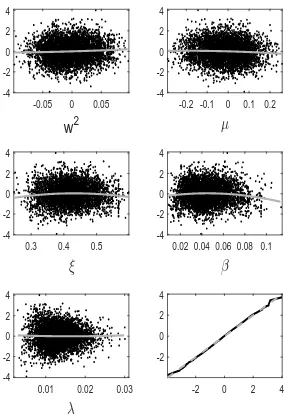
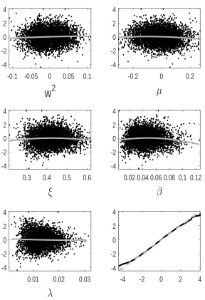
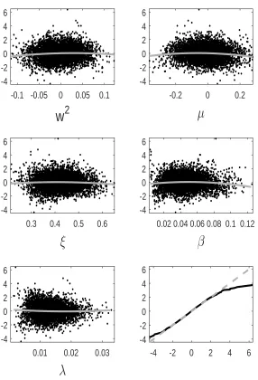
tion error we observe for GP-GIMH. We do this by comparing the GP prediction with other log-likelihood estimates at training points not used to determine the GP fit. Specifically we use the fitted GP from the first run of the MCWM pre-computation step and the training points (and log-likelihood estimates) from the other four MCWM pre-computation runs. The fit is assessed using a standardised residual
ri = ˆ
f(θi)−m∗(θi)
q
s∗(θ i)2+ ˆδ
.
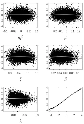
Note that the nugget is included in the GP variance term as the comparisons are made with noisy log-likelihood estimates. In Appendix D, we show normal quantile-quantile plots of the standardised residuals and plots of these residuals against parameter value components. Note that we only include residuals at training points with an accurate GP prediction (standard deviation below) as it is only at these points that the GP prediction alone is used. Appendix D shows the residual plots for different combinations ofandJ. It is evident that the residuals depart further from normality with an increase in . However, from the sensitivity results in Appendix B, it appears that the GP-GIMH method is somewhat robust to the lack of normality in this example. In some cases there is a small amount of curvature in the residuals when plotted against the training samples of each parameter component.
3.2 Gene Network Example
3.2.1 Model and Data
appli-0 10 20 30 40 50 0
5 10 15 20
seconds
observed count
DNA RNA P P
2
Figure 4: Data simulated from the gene network model of Section 3.2.1.
cation. The system is described by eight reactions
DNA + P2
c1DNA×P2
−−−−−−−→DNA·P2, 2P
c5P(P−1)/2
−−−−−−−→P2,
DNA·P2
c2(k−DNA)
−−−−−−−→DNA + P2, P2
c6P2
−−−→2P,
DNA−−−−→c3DNA DNA + RNA, RNA−−−−→ ∅c7RNA ,
RNA c4RNA
−−−−→RNA + P, P c8P
−−→ ∅,
where k is a conservation constant (number of copies of the gene) and c = (c1, . . . , c8) are
the stochastic rate constants governing the speed at which the system evolves. We study the scenario in Golightly and Wilkinson (2005) where data are simulated using rates c = (0.1,0.7,0.35,0.2,0.1,0.9,0.3,0.1), withk= 10, and initial species levels (DNA,RNA,P,P2) =
(5,8,8,8). We simulate equi-spaced data as the next 100 observations (on all species) recorded at 0.5 unit time intervals (see Figure 4). We now investigate how our method performs in making inferences from these simulated data for the stochastic rate constants. Note that we assume that the conservation constantk and initial species levels are known as this is typical in designed experiments (and is as in Golightly and Wilkinson (2005)). Note that we assume these data are observed without error. Even though the observed counts are small, due to the large number of species, this model does not allow a computationally tractable likelihood function. As in Fearnhead et al. (2014), we take independent half-Cauchy priors for the pa-rameters, with density p(ci) ∝1/(1 + 4c2i), ci >0 for i= 1, . . . ,8. Also, in our analysis, we remove the positivity constraint on the rate parameters by working on the log scale, that is, withθi= logci fori= 1, . . . ,8.
3.2.2 Implementation Details
Here we use σ = 0.6 and N = 6000 for the bootstrap particle filter. As mentioned earlier, the smaller the value of σ the closer the approximate posterior is to the true posterior with the drawback that a larger N is required to estimate the likelihood to a reasonable level of precision. At the true parameter value, the log-likelihood is estimated with a standard deviation of 1.9 when N = 6000. Similar to the previous example, pilot runs of GIMH are used to determine a suitable covariance matrix for a multivariate random walk proposal, which all methods use. For simplicity we start all chains at the true parameter value (unless otherwise stated). We run GIMH for 100K iterations and MCWM for 50K iterations and make available theA = 16 cores. At the true parameter value, the standard deviation of the log-likelihood estimate is roughly 0.75 when using the 16 cores. We also considerN = 4000, 5000 and 8000 for GIMH (70K iterations for N = 8000). For comparison purposes we consider a gold standard GIMH run of 350K iterations (withN = 6000).
For the GP-GIMH algorithm, we use a similar approach to the previous example. We first run the MCWM pre-computation step forL= 2000 iterations. During this step, after an initial 50 iterations, we adapt the covariance matrix of the multivariate normal random walk proposal every 10th iteration. Again we do not use the A = 16 cores in the MCWM pre-computing phase. The maximum log-posterior encountered during the MCWM pre-computation phase is roughly−708 and we do not discard any proposals (the minimum is−789). To investigate the effect of the training sample size,J, we compare the results of using a GP trained on all likelihood estimates from the MCWM pre-computing step with that of a GP trained on the same estimates but after thinning the parameter output by a factor of two, producing training data with (roughly)J = 4000 and J = 2000. The remaining part of GP-GIMH (again 100K iterations) uses the same multivariate normal random walk as GIMH/MCWM. No burn-in phase is used for GP-GIMH (in Section 3.2.4 we consider the impact of using a burn-in phase). We consider values of 1.2, 1.5 and 2 and make the 16 cores available. When the tolerance condition is not met, we obtaindK/Ae batches of A = 16 independent likelihood estimates. We run the full GP-GIMH procedure independently five times for each combination ofJ and
.
Code to implement our method for this example can be found at http://www.runmycode. org/companion/view/2663.
3.2.3 Results
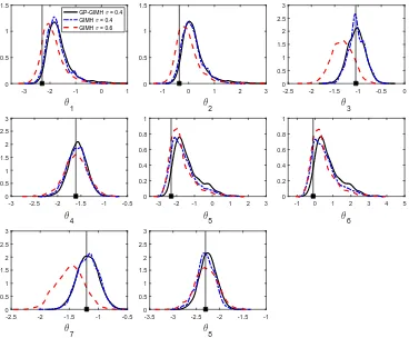
Before discussing posterior approximations, we compare our MCWM training procedure with the history matching approach of Wilkinson (2014). The full details are provided in Appendix E. We find that with less training time our trained GP is able to predict much more accurately than the history matching trained GP for samples from the posterior distribution generated from the exact GIMH method.
As before we find that the GP-GIMH results are generally insensitive to , though we oc-casionally observe incorrect tail behaviour when = 2; see the plots in Appendix F. The marginal posterior density estimates for the different approaches are shown in Figures 5 (with
implemen--3 -2 -1 0 1 θ 1 0 0.5 1 1.5 GP-GIMH GIMH (gold) MCWM
-1 0 1 2 3
θ 2 0 0.5 1 1.5
-2.5 -2 -1.5 -1 -0.5 0
θ 3 0 0.5 1 1.5 2
-3 -2.5 -2 -1.5 -1 -0.5
θ 4 0 0.5 1 1.5 2
-3 -2 -1 0 1 2 3
θ 5 0 0.2 0.4 0.6 0.8 1
-1 0 1 2 3 4 5
θ 6 0 0.2 0.4 0.6 0.8 1
-2.5 -2 -1.5 -1 -0.5
θ 7 0 0.5 1 1.5 2 2.5 3
-3.5 -3 -2.5 -2 -1.5 -1
θ 8 0 0.5 1 1.5 2
Figure 5: Estimated marginal posterior densities for the gene network example from runs of the gold standard GIMH (red dash) and MCWM (blue dash-dot) algorithms and five independent runs of the GP-GIMH (black solid) algorithm with J ≈2000 and= 1.2. The results for GIMH and MCWM are based onN = 6000.
tations use a tolerance of = 1.2. We also show the univariate and bivariate TV distances between the different approximations and the gold standard run in Appendix G. In general it is evident that the GP-GIMH method is producing results not quite as accurate as GIMH but more accurate than MCWM for this example. From the between-run TV distances shown in Appendix G, it is evident that the between-run variability is reduced when increasingJ. Again, for some of the parameters, we see an increase in the between-run TV distances when
= 2.0.
From Table 4 it is evident that GP-GIMH is capturing the true posterior correlation matrix quite accurately. In the GIMH run, there is a period where the Markov chain does not move for roughly 1700 iterations, which highlights the difficulty encountered with the GIMH approach. With the GP-GIMH method, as long as is set low enough, we do not observe such sticking behaviour. Trace plots from the different approaches are shown in Appendix H.
-3 -2 -1 0 1 θ 1 0 0.5 1 1.5 GP-GIMH GIMH (gold) MCWM
-1 0 1 2 3
θ 2 0 0.5 1 1.5
-2.5 -2 -1.5 -1 -0.5 0
θ 3 0 0.5 1 1.5 2
-3 -2.5 -2 -1.5 -1 -0.5
θ 4 0 0.5 1 1.5 2
-3 -2 -1 0 1 2 3
θ 5 0 0.2 0.4 0.6 0.8 1
-1 0 1 2 3 4 5
θ 6 0 0.2 0.4 0.6 0.8 1
-2.5 -2 -1.5 -1 -0.5
θ 7 0 0.5 1 1.5 2
-3.5 -3 -2.5 -2 -1.5 -1
θ 8 0 0.5 1 1.5 2
[image:21.612.122.488.109.413.2]Figure 6: Estimated marginal posterior densities for the gene network example from runs of the gold standard GIMH (red dash) and MCWM (blue dash-dot) algorithms and five independent runs of the GP-GIMH (black solid) algorithm withJ ≈4000 and= 1.2.
Table 4: Upper triangular part of the posterior correlation matrix for θ obtained from the gold standard GIMH/GP-GIMH (first run with J ≈ 2000 and = 1.2) algorithms for the gene network model.
θ2 θ3 θ4 θ5 θ6 θ7 θ8
θ1 0.98/0.97 0.03/0.06 0.00/-0.02 -0.01/-0.04 0.00/-0.04 0.03/0.06 -0.01/0.01
θ2 0.03/0.05 0.00/-0.01 -0.01/-0.04 -0.01/-0.04 0.04/0.05 -0.01/0.02
θ3 -0.01/0.02 -0.01/-0.07 -0.01/-0.07 0.70/0.71 -0.02/-0.01
θ4 0.00/0.06 0.01/0.07 -0.01/-0.02 0.70/0.73
θ5 0.99/0.99 0.00/-0.04 0.01/0.09
θ6 0.00/-0.04 0.01/0.09
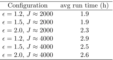
Table 5: Average run times for GP-GIMH (excluding the MCWM pre-computing phase and GP fitting) for different combinations ofJ and for the gene network example. The average time for GP training and fitting is around 4 hours.
Configuration avg run time (h)
= 1.2, J ≈2000 1.9
= 1.5, J ≈2000 1.9
= 2.0, J ≈2000 2.3
= 1.2, J ≈4000 2.9
= 1.5, J ≈4000 2.5
= 2.0, J ≈4000 2.6
Table 6: Comparison of the computational and statistical efficiency of the GIMH, GP-GIMH and MCWM algorithms for the gene network model. For GP-GIMH the results are averaged over the five independent runs for each combination ofJ and . † 70K iterations are used for GIMH whenN = 8000.
method acc rate (%) min ESS avg ESS time (hrs) min ESS/time avg ESS/time
GIMH (N = 4000) 7 517 700 58 9 12
GIMH (N = 5000) 9 689 902 78 9 12
GIMH (N = 6000) 10 537 984 108 5 9
GIMH (N = 8000)† 12 684 944 123 6 8
MCWM 19 445 769 121 4 6
J ≈2000, = 1.2 13 956 1452 5.9 176 260
J ≈2000, = 1.5 13 868 1389 5.9 149 240
J ≈2000, = 2.0 13 495 1190 6.3 81 194
J ≈4000, = 1.2 13 892 1419 7.1 132 206
J ≈4000, = 1.5 13 971 1476 6.7 151 226
J ≈4000, = 2.0 13 716 1354 6.8 110 204
increase in time for GP prediction is offset by the fact that the GP is trained at more points so that unreliable GP predictions (with s∗(θ∗) > ) occur less often. Furthermore, there is lower variability in the run times withJ ≈4000: in the 15 runs of GP-GIMH withJ ≈4000 (five independent runs for each of three different values) the standard deviation of the run time is 0.9 hours whereas the corresponding number forJ ≈2000 is 1.3 hours.
The computational, statistical and overall efficiency of the different approaches is shown in Table 6. Again it is clear that the GP-GIMH algorithm offers generally at least an order of magnitude improvement in overall efficiency, resulting from the large reduction in computing time and a slightly higher acceptance rate than GIMH. The overall efficiency for GP-GIMH depends little onJ in this example. There is perhaps a slight decrease in overall efficiency as
increases, especially for = 2. We also run the GP-GIMH method with 5 different Markov chain starting values (obtained from the MCWM pre-computation step) and obtain similar efficiency results (based on run 1 withJ ≈4000 and∈ {1.2,2.0}).
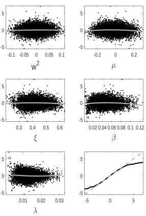
assumption of the residuals is increasingly violated with an increase in . Again there is a small amount of curvature in some of the residual plots, however generally the GP appears to fit reasonably well.
3.2.4 Increasing Accuracy with GP-GIMH
Finally, we attempt to use the increased efficiency of the GP-GIMH approach to target a smaller value ofσ. The idea is to obtain an approximate solution to a more accurate posterior (in the sense that it is closer to the true posterior) rather than an exact solution to a less accurate posterior. Here we setσ = 0.4 and use N = 10000 for the MCWM pre-computing step. Given the challenging nature of this problem, we use the 16 cores in the MCWM pre-computing step to obtain a more accurate log-likelihood estimate at each iteration of the MCWM phase by taking the average of 16 independent likelihood estimates. Using the 16 cores, the log-likelihood estimate has a standard deviation of roughly 2.2 at the true parameter value. The MCWM pre-computing phase is run for 2000 iterations with an adaptive MCMC strategy as detailed earlier. None of the training samples are discarded. We use = 1.2 for the remaining GP-GIMH algorithm with a multivariate normal proposal estimated from a few pilot runs of the method. Once the proposal distribution is determined, GP-GIMH is run for 100K iterations.
Given that all 16 cores are already used to obtain a single log-likelihood estimate, additional likelihood estimates required when s∗(θ∗) > can only be obtained in batches of size 1, increasing the time needed to generate these additional likelihood estimates (compounded by the fact that we use the larger N = 10000 to accommodate the smaller σ). Given the complexity of this application, we examine the impact of including for the first time a burn-in phase. Here we use B= 20000.
Since the likelihood cannot be estimated accurately even with the 16 cores here, GIMH does not perform well with N = 10000 (acceptance rate of 6% over 10K iterations). Instead we trial GIMH using N = 14000 (with this choice the standard deviation of the log-likelihood estimate is roughly 1.6 at the true value).
For GP-GIMH, the MCWM phase takes 10 hours. The remaining part of the GP-GIMH algorithm takes 7.5 hours without the burn-in phase and 2.3 hours with the burn-in phase. The improvement in computing time afforded with the burn-in is however reduced in that 20K less iterations can be used for inference. Using the burn-in period would be even more beneficial if more iterations were performed. Appendix J shows that the posterior estimates obtained by GP-GIMH depend very little on whether a burn-in is used. The GIMH method takes roughly 470 hours to run only 100K iterations. Further, there is a dramatic reduction in acceptance rate, down from 35% for GP-GIMH to 12% for GIMH (note that this is even with smaller random walk standard deviations to improve the acceptance rate). This amounts to an efficiency improvement of roughly 100 times for GP-GIMH (with and without the burn-in).
-3 -2 -1 0 1 θ 1 0 0.5 1 1.5
GP-GIMH σ = 0.4 GIMH σ = 0.4 GIMH σ = 0.6
-1 0 1 2 3
θ 2 0 0.5 1 1.5
-2.5 -2 -1.5 -1 -0.5 0
θ 3 0 0.5 1 1.5 2 2.5 3
-3 -2.5 -2 -1.5 -1 -0.5
θ 4 0 0.5 1 1.5 2 2.5 3
-3 -2 -1 0 1 2 3
θ 5 0 0.2 0.4 0.6 0.8 1
-1 0 1 2 3 4 5
θ 6 0 0.2 0.4 0.6 0.8 1
-2.5 -2 -1.5 -1 -0.5
θ 7 0 0.5 1 1.5 2 2.5 3
-3.5 -3 -2.5 -2 -1.5 -1
[image:24.612.121.489.90.394.2]θ 8 0 0.5 1 1.5 2 2.5 3
Figure 7: Estimated marginal posterior densities for the gene network example from GIMH with σ = 0.6 (red dash) and GP-GIMH with σ = 0.4 and a burn-in phase of B = 20000 iterations (black solid).
accurately. There is a gain in precision forθ4 andθ8, which GP-GIMH is also able to capture.
The GP-GIMH approach is recovering the skewed posteriors (θ1, θ2, θ7 and θ8) with less
accuracy, with the method appearing to spend too much time in the right tails. Overall, the GP-GIMH method is performing well here given the massive improvement in efficiency. The results of GIMH suggest that the posteriors are moving away from the true parameter values forθ1 and θ2 when σ is reduced. This might be explained by the fact that only a relatively
small (partially observed) dataset is used here, and so the parameter values most favourable for the dataset generated may be away from the true parameter values.
4
Discussion
Other choices for the mean function, covariance function and observation model may be selected. Such selections are likely to be problem dependent, for example some noisy log-likelihood functions might be better modelled with an error variance that depends onθ, such as heteroscedastic GP models (Goldberg et al., 1998; Kersting et al., 2007). In practice one may use a model selection procedure (Rasmussen and Williams, 2006, chap. 5) to determine the most appropriate GP for a given training sample. J¨arvenp¨a¨a et al. (2016) use a GP with input-dependent noise for ABC and discuss model selection in this context. However, a more sophisticated GP will result in more complex computations involving the GP. This requires further investigation.
In this article we have not investigated the optimal standard deviation of the log-likelihood estimator to use in the MCWM pre-computing phase. Such an investigation would require an extensive and significant simulation study. Here we found success when the standard deviation of the log-likelihood estimator is roughly 2 in the MCWM pre-computing phase. This is of interest as it is larger than that recommended for GIMH (Doucet et al., 2015), which suggests that our approach should be useful in complex scenarios.
Here we used a multivariate normal random walk proposal in the MCMC. Alternatively, the pre-computed approximation to the log-likelihood could also be used to design improved proposals for GP-GIMH. The covariance function of the GP could be viewed as a smoothed representation of the geometry of the parameter space. Where there is strong dependence between parameters, information such as gradient and curvature can be utilised to propose large moves with high acceptance probability. For example, Zhang et al. (2017) incorporate a pre-computation step in their approximate Hamiltonian Monte Carlo method (see also Rasmussen (2003)).
Our approach could also be used to accelerate approximate Bayesian inferences when an expensive biased likelihood estimator is used. Alquier et al. (2016) present a noisy MCMC framework that provides bounds on the error when a biased likelihood estimator is used in an MCMC method. Another example is the synthetic likelihood of Wood (2010) (see also Price et al. (2017)), which assumes a multivariate normal approximation for the likelihood of a summary statistic, with a mean and covariance matrix estimated by repeated model simulation.
A GP surrogate may be incorporated into delayed-acceptance MCMC to facilitate exact Bayesian inferences in the presence of models where only an unbiased likelihood estimator is available or those with expensive likelihood functions. There is scope here to adapt the GP during the MCMC algorithm by adding training samples when necessary and/or re-estimating hyperparameters.
Acknowledgements
CCD was supported by an Australian Research Council’s Discovery Early Career Researcher Award funding scheme (DE160100741). MTM was supported by the UK Engineering and Physical Sciences Research Council as part of a programme grant (EP/K014463/1). The authors are grateful to Andy Golightly for useful comments on an earlier draft. The authors are also grateful to an Associate Editor and two referees for their helpful suggestions that led to improvements in the presentation and content of this paper.
References
Alquier, P., Friel, N., Everitt, R., and Boland, A. (2016). Noisy Monte Carlo: Convergence of Markov chains with approximate transition kernels. Statistics and Computing, 26(1):29–47.
Andrieu, C., Doucet, A., and Holenstein, R. (2010). Particle Markov chain Monte Carlo methods. Journal of the Royal Statistical Society: Series B (Statistical Methodology), 72(3):269–342.
Andrieu, C. and Roberts, G. O. (2009). The pseudo-marginal approach for efficient Monte Carlo computations. The Annals of Statistics, 37(2):697–725.
Baggaley, A. W., Boys, R. J., Golightly, A., Sarson, G. R., and Shukurov, A. (2012). In-ference for population dynamics in the neolithic period. The Annals of Applied Statistics, 6(4):1352–1376.
Beaumont, M. A. (2003). Estimation of population growth or decline in genetically monitored populations. Genetics, 164(3):1139–1160.
B´erard, J., Del Moral, P., and Doucet, A. (2014). A lognormal central limit theorem for parti-cle approximations of normalizing constants. Electronic Journal of Probability, 19(94):1–28.
Carson, J., Crucifix, M., Preston, S., and Wilkinson, R. D. (2017). Bayesian model selection for the glacial-interglacial cycle. To appear in Journal of the Royal Statistical Society: Series C (Applied Statistics).
Chopin, N., Jacob, P. E., and Papaspiliopoulos, O. (2013). SMC2: an efficient algorithm for sequential analysis of state space models. Journal of the Royal Statistical Society: Series B (Statistical Methodology), 75(3):397–426.
Christen, J. A. and Fox, C. (2005). Markov chain Monte Carlo using an approximation. Journal of Computational and Graphical Statistics, 14(4):795–810.
Conrad, P. R., Marzouk, Y. M., Pillai, N. S., and Smith, A. (2016). Accelerating asymptoti-cally exact MCMC for computationally intensive models via local approximations. Journal of the American Statistical Association, 111(516):1591–1607.
Drovandi, C. C. (2014). Pseudo-marginal algorithms with multiple CPUs. http://eprints.qut.edu.au/61505/.
Drovandi, C. C. and McCutchan, R. A. (2016). Alive SMC2: Bayesian model selection for low-count time series models with intractable likelihoods. Biometrics, 72(2):344–353.
Duan, J.-C. and Fulop, A. (2015). Density-tempered marginalized sequential Monte Carlo samplers. Journal of Business & Economic Statistics, 33(2):192–202.
Fearnhead, P., Giagos, V., and Sherlock, C. (2014). Inference for reaction networks using the linear noise approximation. Biometrics, 70(2):457–466.
Goldberg, P. W., Williams, C. K. I., and Bishop, C. M. (1998). Regression with input-dependent noise: a Gaussian process treatment. In Advances in Neural Information Processing Systems (NIPS), volume 10, pages 493–499. The MIT Press.
Golightly, A., Henderson, D. A., and Sherlock, C. (2015). Delayed acceptance particle MCMC for exact inference in stochastic kinetic models. Statistics and Computing, 25(5):1039–1055.
Golightly, A. and Wilkinson, D. J. (2005). Bayesian inference for stochastic kinetic models using a diffusion approximation. Biometrics, 61(3):781–788.
Gordon, N. J., Salmond, D. J., and Smith, A. F. M. (1993). Novel approach to nonlinear/non-Gaussian Bayesian state estimation. In Radar and Signal Processing, IEE Proceedings F, volume 140, pages 107–113.
Gutmann, M. U. and Corander, J. (2016). Bayesian optimization for likelihood-free inference of simulator-based statistical models. Journal of Machine Learning Research, 17(1):4256– 4302.
Henderson, D. A., Boys, R. J., Krishnan, K. J., Lawless, C., and Wilkinson, D. J. (2009). Bayesian emulation and calibration of a stochastic computer model of mitochondrial dna deletions in substantia nigra neurons. Journal of the American Statistical Association, 104(485):76–87.
Henderson, D. A., Boys, R. J., and Wilkinson, D. J. (2010). Bayesian calibration of a stochastic kinetic computer model using multiple data sources. Biometrics, 66(1):249–256.
Holenstein, R. (2009). Particle Markov Chain Monte Carlo. PhD thesis, The University Of British Columbia.
J¨arvenp¨a¨a, M., Gutmann, M., Vehtari, A., and Marttinen, P. (2016). Gaussian process mod-eling in approximate Bayesian computation to estimate horizontal gene transfer in bacteria. arXiv:1610.06462 [stat.ML]. arXiv preprint.
Kennedy, M. C. and O’Hagan, A. (2000). Predicting the output from a complex computer code when fast approximations are available. Biometrika, 87(1):1–13.
Kersting, K., Plagemann, C., Pfaff, P., and Burgard, W. (2007). Most likely heteroscedas-tic Gaussian process regression. In Proceedings of the 24th International Conference on Machine Learning (ICML), volume 227 of ACM International Conference Proceeding Series, pages 393–400.
Medina-Aguayo, F. J., Lee, A., and Roberts, G. O. (2016). Stability of noisy Metropolis– Hastings. Statistics and Computing, 26(6):1187–1211.
Meeds, E. and Welling, M. (2014). GPS-ABC: Gaussian process surrogate approximate Bayesian computation. In Proceedings of the 30th Conference on Uncertainty in Artificial Intelligence (UAI), pages 593–602, Quebec City, Canada.
Plummer, M., Best, N., Cowles, K., and Vines, K. (2006). CODA: Convergence diagnosis and output analysis for MCMC. R News, 6(1):7–11.
Price, L. F., Drovandi, C. C., Lee, A., and Nott, D. J. (2017). Bayesian synthetic likelihood. Journal of Computational and Graphical Statistics, doi: 10.1080/10618600.2017.1302882.
Rasmussen, C. E. (2003). Gaussian processes to speed up hybrid Monte Carlo for expensive Bayesian integrals. In Bernardo, J., Bayarri, M., Berger, J., Dawid, A., Heckerman, D., Smith, A., and West, M., editors, Bayesian Statistics, volume 7, pages 651–659.
Rasmussen, C. E. and Williams, C. K. I. (2006). Gaussian processes for machine learning. The MIT Press, Cambridge, Massachusetts.
Sherlock, C., Golightly, A., and Henderson, D. A. (2017). Adaptive, delayed-acceptance MCMC for targets with expensive likelihoods. Journal of Computational and Graphical Statistics, 26(2):434–444.
Tran, M.-N., Nott, D. J., and Kohn, R. (2017). Variational Bayes with intractable likelihood. To appear in Journal of Computational and Graphical Statistics.
Tran, M.-N., Scharth, M., Pitt, M. K., and Kohn, R. (2014). Importance sampling squared for Bayesian inference in latent variable models. Available at SSRN 2386371.
Wilkinson, R. (2014). Accelerating ABC methods using Gaussian processes. Journal of Machine Learning Research, 33:1015–1023.
Wood, S. N. (2010). Statistical inference for noisy nonlinear ecological dynamic systems. Nature, 466:1102–1107.
Appendices for Accelerating Pseudo-Marginal MCMC using Gaussian
Processes
C. C. Drovandi*, M. T. Moores† and R. J. Boys‡
*Australian Centre of Excellence for Mathematical and Statistical Frontiers and Queensland University of Technology, Brisbane, Australia 4001
† University of Warwick, Coventry CV4 7AL, United Kingdom
‡ Newcastle University, Newcastle upon Tyne NE1 7RU, United Kingdom
email: [email protected]
A
GIMH and MCWM algorithms
The pseudo-marginal algorithms discussed in the main text are shown in Algorithm 1 (GIMH) and Algorithm 2 (MCWM).
Algorithm 1 GIMH algorithm of Beaumont (2003).
Input: θ0 and iters
Output: MCMC outputθ1, . . . ,θiters
1: Compute φ0= ˆp(y|θ0)
2: fori= 1 toiters do
3: Propose θ∗∼q(·|θi−1)
4: Compute φ∗ = ˆp(y|θ∗)
5: Compute α= min
n
1, φ∗p(θ
∗
)q(θi−1|θ∗) φi−1p(θi−1)q(θ∗|θi−1)
o
6: Draw u∼ U(0,1)
7: if u < α then
8: Setφi=φ∗ and θi =θ∗
9: else
10: Setφi=φi−1 and θi =θi−1
11: end if
12: end for
Algorithm 2 MCWM algorithm of Beaumont (2003).
Input: θ0 and iters
Output: MCMC outputθ1, . . . ,θiters
1: Compute φ0= ˆp(y|θ0)
2: fori= 1 toiters do
3: Compute φi−1 = ˆp(y|θi−1)
4: Propose θ∗∼q(·|θi−1)
5: Compute φ∗ = ˆp(y|θ∗)
6: Compute α= minn1, φ∗p(θ∗)q(θi−1|θ∗)
φi−1p(θi−1)q(θ∗|θi−1)
o
7: Draw u∼ U(0,1)
8: if u < α then
9: Setθi =θ∗
10: else
11: Setθi =θi−1
12: end if
B
Sensitivity of GP-GIMH to
for the stochastic volatility example
-0.1
-0.05
0
0.05
0.1
w
2
0
10
20
30
-0.4
-0.2
0
0.2
µ
0
5
10
0.2
0.3
0.4
0.5
0.6
ξ
0
5
10
15
0
0.05
0.1
0.15
β
0
20
40
60
0
0.01
0.02
0.03
λ
0
50
100
150
Figure 1: Sensitivity tofor the stochastic volatility example for the first independent run whenJ ≈1500.
-0.1
-0.05
0
0.05
0.1
w
2
0
10
20
30
-0.4
-0.2
0
0.2
µ
0
5
10
0.2
0.3
0.4
0.5
0.6
ξ
0
5
10
15
0
0.05
0.1
0.15
β
0
20
40
0
0.01
0.02
0.03
λ
0
50
100
150
Figure 2: Sensitivity to for the stochastic volatility example for the second independent run when
-0.1
-0.05
0
0.05
0.1
w
2
0
10
20
30
-0.4
-0.2
0
0.2
µ
0
5
10
0.2
0.3
0.4
0.5
0.6
ξ
0
5
10
15
0
0.05
0.1
0.15
β
0
20
40
60
0
0.01
0.02
0.03
λ
0
50
100
150
Figure 3: Sensitivity tofor the stochastic volatility example for the third independent run whenJ ≈1500.
-0.1
-0.05
0
0.05
0.1
w
2
0
10
20
30
-0.4
-0.2
0
0.2
µ
0
5
10
0.2
0.3
0.4
0.5
0.6
ξ
0
5
10
15
0
0.05
0.1
0.15
β
0
20
40
60
0
0.01
0.02
0.03
λ
0
[image:34.612.140.475.139.613.2]50
100
150
Figure 4: Sensitivity to for the stochastic volatility example for the fourth independent run when