Is the ring inside or outside the planet?: the effect of planet migration
on dust rings
Farzana Meru ,
1,2,3‹Giovanni P. Rosotti ,
3Richard A. Booth ,
3Pooneh Nazari
3,4and Cathie J. Clarke
31Department of Physics, University of Warwick, Gibbet Hill Road, Coventry CV4 7AL, UK
2Centre for Exoplanets and Habitability, University of Warwick, Gibbet Hill Road, Coventry CV4 7AL, UK 3Institute of Astronomy, University of Cambridge, Madingley Road, Cambridge CB3 0HA, UK
4SUPA, School of Physics and Astronomy, University of St Andrews, North Haugh, St Andrews, Scotland KY16 9SS, UK
Accepted 2018 October 11. Received 2018 September 25; in original form 2018 March 20
A B S T R A C T
Planet migration in protoplanetary discs plays an important role in the longer term evolution of planetary systems, yet we currently have no direct observational test to determine if a planet is migrating in its gaseous disc. We explore the formation and evolution of dust rings – now commonly observed in protoplanetary discs by the Atacama Large Millimeter/submillimeter Array – in the presence of relatively low-mass (12–60 M⊕) migrating planets. Through 2D hydrodynamical simulations using gas and dust we find that the importance of perturbations in the pressure profile interior and exterior to the planet varies for different particle sizes. For small sizes, a dust enhancement occurs interior to the planet, whereas it is exterior to it for large particles. The transition between these two behaviours happens when the dust drift velocity is comparable to the planet migration velocity. We predict that an observational signature of a migrating planet consists of a significant outwards shift of an observed mid-plane dust ring as the wavelength is increased.
Key words: methods: numerical – planets and satellites: dynamical evolution and stability – planets and satellites: formation – planet–disc interactions – protoplanetary discs.
1 I N T R O D U C T I O N
Our knowledge of protoplanetary discs is being revolutionized by new observational facilities like the Atacama Large Millime-ter/submillimeter Array (ALMA), the Spectro-Polarimetric High-contrast Exoplanet REsearch instrument on the Very Large Tele-scope, and the Gemini Planet Instrument on the Gemini Telescope. These facilities are revealing that most discs, when observed at high resolution, show conspicuous sub-structures at small spatial
scales, such as spirals (e.g. Benisty et al.2015; Wagner et al.2015),
crescents (e.g. van der Marel et al.2013), and rings and gaps (e.g.
ALMA Partnership et al.2015; Rapson et al.2015).
It is very tempting to link these structures to the presence of forming planets in their discs. Indeed, it is well known that plan-ets perturb their natal discs through their gravitational influence
(Goldreich & Tremaine1980). Depending on the planet mass and
the disc conditions, these perturbations have different morphologies explaining, at least in principle, the variety found in observations. These structures can therefore be used as signposts of planets, mak-ing it possible to reconstruct the properties of the unseen planet. In
E-mail:[email protected]
turn, by comparing the results with theoretical expectations we can improve our understanding of planet formation. This information is particularly precious given that, while the detection of exoplanets around main-sequence stars has been highly successful (thousands
of exoplanets are now known1), only a handful of exoplanets have
been detected around pre-main-sequence stars (van Eyken et al.
2012; Ciardi et al. 2015; David et al. 2016; Donati et al. 2016;
Johns-Krull et al.2016; Biddle et al.2018). We also note that
al-ternative mechanisms for spirals (such as gravitational instabilities,
e.g. Kratter & Lodato2016; and shadows, e.g. Montesinos et al.
2016), crescents (such as vortices, e.g. Reg´aly et al.2012; Ataiee
et al.2013; and eccentric planets, e.g. Ataiee et al.2013), rings
and gaps (such as dead zone edges, e.g. Ruge et al.2016; Pinilla
et al.2016, dust processes, e.g. Birnstiel et al.2015; Okuzumi et al.
2016; Pinilla et al.2017; Dullemond & Penzlin2018, and
photoe-vaporation, e.g. Alexander et al.2014; Ercolano et al.2017) have
been proposed. We will not contribute to this particular debate, but
1See the NASA Exoplanet Archive athttps://exoplanetarchive.ipac.caltech. edu/. While the majority of the planets found byKeplerare not confirmed, the false positive probability is estimated to be only 5–10 per cent (Fressin et al.2013; Morton & Johnson2011).
2018 The Author(s)
note that planet formation is an extremely frequent phenomenon (at least 50 per cent of stars have planetary systems, Mayor et al.
2011; Fressin et al.2013). Therefore, while not all observed
struc-tures are necessarily the signposts of planets, it is not inconceivable that at least a subset of the observed structures is due to planets interacting with the protoplanetary disc.
One of the biggest unknowns in planet formation is the role of disc migration. Due to the limited mass available in the inner disc, disc-driven migration is a crucial ingredient of planet formation models
(e.g. Alibert et al.2006) that assemble planetary cores outside the
water snowline and bring them closer to the star (in contrast to the
opposite view ofin situformation, (e.g. Chiang & Laughlin2013).
Migration is for example invoked in the context of the Solar System to explain the asteroid belt and the small mass of Mars (Grand
Tack scenario, Walsh et al.2011). While migration is an old topic
(Goldreich & Tremaine1980), it is far from being well understood
(see Kley & Nelson2012; Baruteau et al.2013for recent reviews).
The least understood regime is the so-called Type I migration, valid for planets up to roughly Neptune mass. In this range of planet masses migration is calculated to be fast (with typical timescales of
≈O(100) orbits), yet very sensitive to the disc conditions close to the
planet (Paardekooper, Baruteau & Kley2011; Bitsch et al.2014a),
making theoretical predictions a challenge: even the direction of migration is unclear.
This issue calls for observational benchmarks, which are cur-rently lacking. Since we only see the end product of planet forma-tion around main-sequence stars, migraforma-tion cannot be disentangled from the other phenomena affecting planet formation. For example,
while hot Jupiters might be seen as evidence of disc migration2
(Lin, Bodenheimer & Richardson1996), they could also be
pro-duced by dynamical scattering after the disc has dispersed (Rasio &
Ford1996). As another example, while the abundance of planets
observed near mean motion resonances in theKeplermultiplanet
population (Lissauer et al.2011) is suggestive of migration (Lee &
Peale2002), it could also be explained by tidal interactions between
planets (Lithwick & Wu2012).
In this paper, we investigate the observational signatures of plan-ets undergoing migration in protoplanetary discs. We focus on ax-isymmetric structures, i.e. gaps and rings, now commonly observed by ALMA. The most well-known example is the disc around the
young star HL Tau (ALMA Partnership et al.2015), but ALMA is
revealing that many other discs show rings: HD163296 (Isella et al.
2016), Tw Hya (Andrews et al.2016), HD97048 (van der Plas et al.
2017), HD169142 (Fedele et al.2017), AS 209 (Fedele et al.2017),
Elias 24 (Dipierro et al.2018), CI Tau (Clarke et al.2018) and many
more (Long et al.2018).
A number of authors have shown, starting from the seminal work
of Paardekooper & Mellema (2004), that relatively low-mass planets
can open gaps and rings in the dust, and are observable with ALMA. This is in contrast to other structures such as spirals and vortices that require planets with masses comparable or even higher than
Jupiter (Juh´asz et al.2015; Dong & Fung2017; de Val-Borro et al.
2007). In particular, Rosotti et al. (2016) quantified the threshold
for gap opening in the dust to be≈10M⊕for typical disc
param-eters (see also the dust gap opening criterion of Dipierro & Laibe
2017). However, planet migration has either not been included in
2We know however of at least one case (the star CI Tau) in which the hot Jupiter is likely to have been produced via disc migration since the system still possesses a protoplanetary disc (Johns-Krull et al.2016; Rosotti et al.
2017).
these models, such that a stationary planet on a fixed circular or-bit has been assumed, or the simulations have not involved planets migrating to a significant extent. Migration is particularly important since planets that have not opened a gap in the gas are believed to undergo fast Type I migration.
In this paper, we study how planet migration influences the for-mation of gaps and rings, and whether we can use the recent ob-servations previously discussed to put observational constraints on planetary migration. We shall see that migrating planets create rings inside or outside their orbit depending on the dust size. Since the emissivity of dust grains depends on the maximum grain size in the mixture, this in principle means that multiwavelength imaging could reveal the differential concentration of grains of different sizes in different structures, thus offering an observational test to assess whether a planet is migrating.
In Section 2, we describe our method and simulation set-up. In Section 3, we show the effect of migration on the gas and dust separately. We discuss our findings and conclude in Sections 4 and 5, respectively.
2 M E T H O D
2.1 Numerical method
We run 2D multifluid simulations where we evolve the dust and
gas at the same time using theFARGO-3Dcode (Ben´ıtez-Llambay &
Masset2016). The algorithm is well tested and has been used many
times for protoplanetary disc studies (see de Val-Borro et al.2006for
an algorithmic comparison). The code solves the mass, momentum, and energy equations of hydrodynamics:
∂
∂t + ∇ ·(u) (1)
∂u
∂t +u· ∇u+ ∇p
= g (2)
and
∂e
∂t +u· ∇e+ p
∇ ·u=0, (3)
whereis the disc surface mass density,u,e, andpare the gas
velocity, specific internal energy, and pressure, andgis the gravity
term.
As described in detail in Rosotti et al. (2016), theFARGO-3Dgas
hydrodynamics code has been extended to include dust, treating the dust as a pressureless fluid that is coupled to the gas via linear drag
forces. The equation for the dust velocity,vd, is given by
dvd
dt +vd· ∇vd= −
1 ts
(vd−u(t))+ad (4)
where ad are the non-drag accelerations felt by the dust and ts
is the stopping time. We employ a semi-implicit time integra-tion algorithm for the dust, which has the advantage that it does not require short time-steps even when dealing with tightly cou-pled dust. These approximations are valid for low dust-to-gas
ra-tios and particles with Stokes number St 1 (Garaud,
Barri`ere-Fouchet & Lin 2004). The effect of dust on the gas has been
neglected.
We use 2D cylindrical coordinates with 1024 and 440 uniformly spaced cells in the azimuthal and radial directions, respectively. With this resolution the planet’s Hill radius at its initial location
is resolved with ≈4–6 grid cells. We also perform a resolution
test whereby we double the number of grid cells in each direction to show that the main result presented in this paper still holds (Appendix C). We use dimensionless units in which the orbital
radius of the planet (Rp) is initially at unity and the unit of mass is
that of the central star, while the unit of time is the inverse of the
Keplerian frequency of the planet atRp=1. We use non-reflecting
boundary conditions at both boundaries for the gas. While Rosotti
et al. (2016) fixed the dust density to its initial value at the inner
boundary, here we allow the dust density to drop below this. To this end, we use a power-law extrapolation of the dust density at the inner boundary, limiting its value to be no more than the initial value to avoid generating arbitrary amounts of dust at the inner boundary.
Along with the gas dynamics, we integrate the evolution of the dust in response to the gas disc structure. To keep our simulations scale-free we fix the Stokes number, St, of the grains rather than their physical size. We use five dust sizes with logarithmically spaced
Stokes numbers: 2×10⁻³, 6×10⁻³, 2×10⁻², 6×10⁻², and
0.2.
2.2 Simulation set-up
We model a disc that extends fromR=0.2 to 3 using the exact same
initial surface mass density and temperature structures as Rosotti
et al. (2016). The disc surface mass density is given by
(R)=0
R0
R, (5)
where0=1×10⁻³in code units andR0=1. Note that the value
of0is arbitrary as the simulations are scale-free. Nevertheless as
an example, to put this into context, for a 1M central star and
initial planet location of 10 au, this translates to0=888 g cm−2
at 1 au. We model a locally isothermal disc structure so that the temperature profile does not change over time, setting the aspect ratio to be
H R =0.05
R R0
0.25
. (6)
We use theαviscviscosity prescription of Shakura & Sunyaev (1973)
withαvisc=10−3. Since we do not include the dust backreaction on
to the gas, the absolute normalization of the dust density is arbitrary and the results can be rescaled to any choice of the initial dust-to-gas ratio. For simplicity, we use the same surface density normalization for the dust as for the gas.
2.2.1 Calibration of the migration rate
We model planets with planet-to-star mass ratios ofq=3.6×10⁻⁵,
6×10⁻⁵, 9×10⁻⁵, and 1.8×10⁻⁴which for a 1M
central star
translates to planet masses ofMp=12, 20, 30, and 60M⊕. We first
run the simulations allowing the planets to migrate naturally under the influence of the disc torques. We measure their Type I migration
time-scale,τI, by fitting the following relation that describes the
decay of the planet semimajor axis as
Rp=Rp,0e−t/τI (7)
We then repeat the simulations in a controlled way where the planet does not feel the effects of the disc but instead has its migration
rate prescribed according to its measured value ofτIin equation (7)
(akin to the simulations performed by Duffell et al.2014). We
[image:3.595.307.546.93.167.2]con-firm that the radial migration of the planet in the disc using this
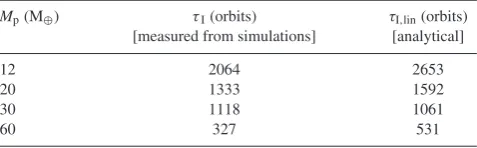
Table 1. Table showing the migration time-scale,τI, as measured from the simulations and the analytical values given by equation (8). The measured values are within a factor of 2 of the analytical estimates.
Mp(M⊕) τI(orbits) τI,lin(orbits)
[measured from simulations] [analytical]
12 2064 2653
20 1333 1592
30 1118 1061
60 327 531
approach is similar to that of the planet migrating freely, though it is worth mentioning that equation (7) starts to deviate from the
actual migration tracks for higher planet masses (60 M⊕). While
this could, in principle, affect the pressure profile for the 60 M⊕
planet, and hence the dust collection, the main qualitative results presented in this paper are unaffected by the use of a prescribed migration (see end of this section). Unless specified, all simulations are performed with the planet migrating at a prescribed rate that is roughly equivalent to the Type I rate though we also run some simu-lations with different migration rates. We confirm that the values of
τIare within a factor of 2 of the values expected from linear theory,
τI,lin, (Table1) using
τI,lin=
R2 ppMp
2p
, (8)
wherepis the Keplerian velocity evaluated at the planet’s location
and
p=
1 γ
−2.5−1.7β+0.1α+1.1
3
2−α
+7.9ξ
γ
×q h
2
pRp4 2
p (9)
is the torque exerted on the planet evaluated using equation (47) of
Paardekooper et al. (2010), whereγ is the ratio of specific heats,
−αand −β are the slopes of the disc surface mass density and
temperature profiles respectively, andξ=β−(γ −1)α.
Given our choice to specifically explore the effects of Type I migration, we essentially assign these simulations a scale, though note that these simulations are in fact valid for any disc mass for the migration rate prescribed in our simulations. The main results pre-sented in this paper involve simulations where the planet is placed in the disc at the specified mass and allowed to migrate immediately at the prescribed rate. We also tested planets that are held on a fixed orbit before migrating as well as those allowed to freely migrate un-der the disc’s natural torques and confirm that the qualitative result presented in this paper still holds.
3 R E S U LT S
3.1 The effect of migration on the gas
Here, we consider how migration affects the pressure profile around
the planet. For St<1 there are two ways in which the perturbed
pressure profile can give rise to rings and gaps in the dust density, as
identified by Rosotti et al. (2016). First, if the pressure perturbation
is strong enough to create a local maximum in the pressure profile, then dust drifting towards the maximum will be trapped there as the sign of the radial drift velocity, given by
vdrift= −
ηvk
St+St−1 =
H R
2
vk
∂logP ∂logR
1
St+St−1, (10)
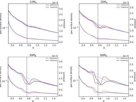
Figure 1. Gas surface density (solid lines) and pressure (dashed lines) profiles for 12, 20, 30, and 60 M⊕planets atRp=0.75. The stationary planet is in red and the migrating planet is in blue. The dotted line shows the initial surface density profile. The effect of migration is first to reduce the effect of the planet’s perturbation on the gas disc exterior to the planet, and secondly to modify the pressure perturbation interior to it for low-mass planets. The magenta line in the top right panel shows the gas profile for a planet migrating approximately three times faster than the Type I rate.
changes at the pressure maximum.3The Keplerian velocity is given
byvk. Secondly, there can be a point of inflection where the pressure
perturbation is too small to create a pressure maximum but is where the absolute pressure gradient is a minimum and thus the dust drift velocity is the slowest as the dust migrates inwards. If the flow is in a steady state, mass conservation implies that the density will reach a maximum there. This phenomenon was termed a ‘traffic jam’ by
Rosotti et al. (2016).
Fig. 1shows the gas surface density and pressure profiles for
the migrating and stationary planet simulations, and shows that migration affects the pressure profile inside and outside the planet in different ways. First, the pressure maximum outside the planet is weaker. Secondly for low-mass migrating planets (12, 20, and 30
M⊕), the point of inflection in the pressure profileinteriorto the
planet is more pronounced than in the stationary planet simulations
(this is most obvious in the case of the 20 and 30 M⊕planets).
Fig.2shows the position of the pressure maximum or point of
inflection in the outer and inner discs with respect to the planet’s position (and normalized by the planet’s position, since the planet’s
3This equation breaks down when the deviation of the gas angular velocity from Keplerian is dominated by the planet, rather than the pressure gradient, which occurs within a few Hill radii of the planet. This also assumes steady state, which is reasonable for St<1 (Dipierro & Laibe2017).
semimajor axis also influences the location). A horizontal line on this graph would show that the pressure trap moves with the planet.
With the exception of the 30 and 60 M⊕ cases at the start of the
simulations, the pressure traps are located within 25 per cent of the
distance for stationary planets (Rosotti et al.2016), and mostly are
quite close to the stationary planet estimates.4Given that Rosotti
et al. (2016) show that the gap width (and hence location of the
pressure perturbation) scales asM1/3
p , this suggests that the planet
mass estimates based on stationary planets are not likely to be wrong
by more than a factor of two. Note that while Rosotti et al. (2016)
determined their planet mass estimates based on the locations of
pressure maxima with respect to the planet, Fig.2shows that the
mass estimates determined from a dust maximum associated with a point of inflection would be similar. However, there is also a trend with radius, which points to some scale height dependence in
this regime. In addition, we show in Fig.3that the distance of the
pressure perturbation is not as sensitive to the migration speed. In addition to the main pressure maximum that follows the planet,
Fig. 2also shows hints of a secondary pressure maximum that
initially forms outside the location of the planet atR≈1.13, which
can be seen by comparing the location of the pressure maximum to
4At small radii, the results are affected by the resolution and inner boundary.
Figure 2. Relative distance between the location of the planet and the pressure perturbation exterior (left) and interior (right) to the planet for various mass planets migrating fromRp=1. Crosses show times when the planet creates a full pressure maximum, while dots denote times where the magnitude of the pressure gradient is a minimum, but not zero, i.e. a point of inflection exists in the pressure profile. The solid lines show the results determined from fits to non-migrating planets (Rosotti et al.2016) and the dashed black line shows how a fixed maximum atR=1.13 would appear in this plot. For most of the simulation, the pressure perturbations remain with the planet.
Figure 3. As with Fig.2, but for a 20 M⊕planet migrating at the Type I migration rate (green) as well as four times faster (red) and three times slower (blue). Crosses show times when the planet creates a full pressure maximum, while dots denote times where the magnitude of the pressure gradient is a minimum, but not zero, i.e. a point of inflection exists in the pressure profile. The pressure perturbation remains with the planet irrespective of the migration speed.
theRmax≈1.13 line for the 30 and 60 M⊕planets. Note that since
we allow the planet to begin migrating immediately, the feature is not simply a residual gap or pressure maximum opened before the planet starts to migrate. This extra pressure maximum can be seen
clearly in Fig.4, which forms outside the initial location of the
planet, slowly disappearing over time by evolving into a point of inflection. We explain the origin of this feature in Appendix A.
Despite the weaker pressure maximum formed in the outer disc with migrating planets, we find that the planet mass required to produce a maximum in the pressure profile does not change
dra-matically for typical disc masses. Rosotti et al. (2016) found the
minimum mass for creating a pressure maximum in exactly the
same disc set-up as ours to be between 12 and 20 M⊕atH/R=0.05
for non-migrating planets. Similarly, Lambrechts, Johansen &
Mor-bidelli (2014) reported a critical mass of 20(H /(0.05R))3M
⊕, typically called the ‘pebble isolation mass’ because it is the mini-mum mass that forms a pressure maximini-mum exterior to it and
pre-vents the flux of pebbles into the inner disc. Bitsch et al. (2018) and
Ataiee et al. (2018) produce refined criteria for the pebble isolation
mass considering the disc aspect ratio and turbulence. Bitsch et al.
(2018) also include a dependence on the disc’s initial pressure
pro-file. Our results are consistent with the pebble isolation mass from
Lambrechts et al. (2014) and the gas-only simulations (i.e.
equiva-lent to what we present in this section) of Bitsch et al. (2018) and
Ataiee et al. (2018). Fig.1shows that the 20 M⊕planet still forms
an exterior pressure maximum when it migrates at the Type I rate. However, we note that varying the migration rate can change this
– as shown by the red line in the left-hand panel of Fig.3which
shows that a migration rate a few times faster than our standard model results in a point of inflection instead of a maximum.
The flared structure used in our simulations means that the pebble isolation mass varies with radius, and all of the planets eventually create a pressure maximum in the disc once they reach small enough
radii. We demonstrate this for the 12 M⊕ planet in Figs5and2
(left-hand panel), where the transition occurs when the planet is
at aboutR=0.55, whereH/R=0.04. We note that while this is
[image:5.595.61.534.305.486.2]Figure 4. Graph showing how the gas profile changes in the presence of a 60 M⊕planet migrating at the Type I rate. Initially, a single density maximum forms but over time a second density maximum forms, while the first develops into a point of inflection. The dotted lines show the planet location. The planet is initially atRp=1. The axes are in code units.
Figure 5. Time evolution of the pressure profile (normalized by the unper-turbed value atR=1) for the 12 M⊕planet. As the planet migrates inwards, it transitions from creating a point of inflection (traffic jam) to a pressure maximum (dust trap) exterior to the planet due to the decrease in the disc aspect ratio (see Section 3.1). The vertical dashed lines show the location of the planet.
consistent with the pebble isolation mass from Lambrechts et al.
(2014), Bitsch et al. (2018), and Ataiee et al. (2018), this cannot
hold for migrating planets in general. As an example in the 20 M⊕
case, the radius at which the external pressure profile transitions from a point of inflection to a pressure maximum is smaller for
larger migration rates (see Fig.3, left-hand panel). This suggests
that although the effect on the pebble isolation mass is rather minor in the cases studied here, this may not necessarily be the case and so an additional criterion factoring in the migration rate needs to be included into the pebble isolation mass, somewhat analogous to the gap-opening time-scale criterion required for migrating planets
(Lin & Papaloizou1986; Malik et al.2015), and more so for very
fast migrating planets (e.g. in the Type III regime). Furthermore, we note that although more massive planets migrate more quickly in the Type I regime, they still open deeper gaps than less massive planets. This is a consequence of torques exerted on the disc by the
planet scaling asq2, while the migration speed scales withq. Thus
more massive planets open up deeper gaps, even when their faster migration rate is taken into account.
3.2 The effect of migration on the dust
3.2.1 Overview of dust evolution in the presence of migrating planets
Fig.6shows the surface density of the dust in the presence of a 30
M⊕planet, comparing both the migrating and stationary planet cases
for each dust species considered, as well as the pressure profile. The
behaviour for the 12, 20, and 60 M⊕simulations are similar to the
30 M⊕simulation and where relevant we include additional figures
in Appendix B. The bottom panel of Fig.6and Section 3.1 show
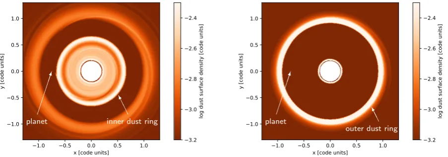
pressure perturbations both interior and exterior to the planet and thus dust can potentially collect in both locations in the migrating planet simulations. This is confirmed by inspecting the dust surface density plots. The large dust sizes always show a peak exterior to the planet. For the smallest dust sizes, there is barely a peak in the dust density exterior to the migrating planet, whereas there is always a peak for the stationary planet case. However, the dust peak interior to the planet is more prominent for the migrating planet simulations. The presence of a ring interior to the planet in small
sizes and exterior to it in large sizes is further highlighted in Fig.7,
which shows the 2D dust surface density distributions for different dust sizes.
Furthermore Fig.8shows that in the migrating planet simulations,
different dust species have their dust density maxima at slightly different locations, whereas for stationary planet simulations the dust maxima are all in a similar location and mostly coincident with the location of the pressure maximum.
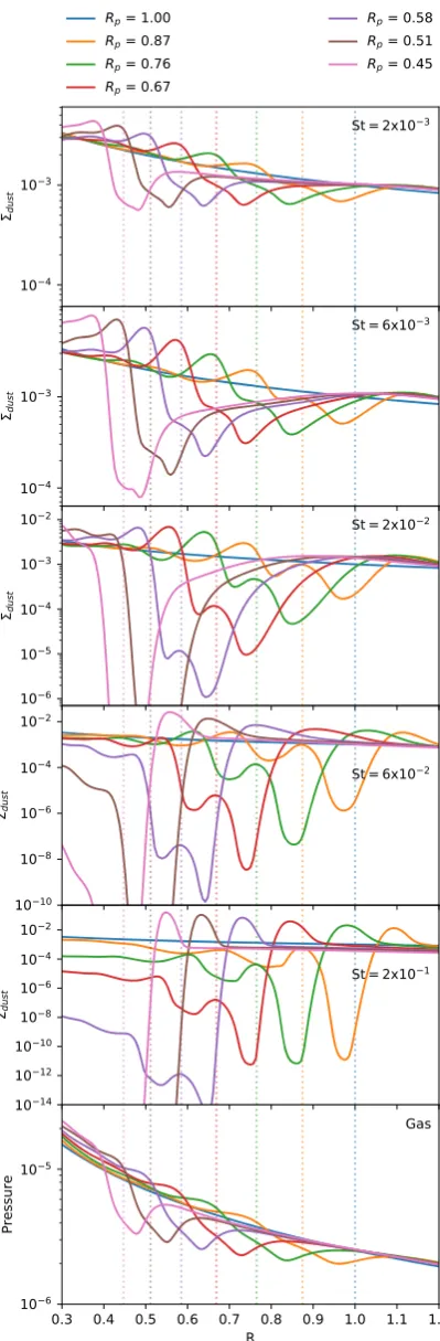
The behaviour of the dust in the presence of a migrating planet
is more obvious when looking at Fig. 9 which shows the time
evolution of each dust size. First, it is clear that for low Stokes
numbers (St<<1), the dust ring is interior to the planet while
for larger Stokes numbers (St∼0.1) it is exterior. Note that an
interior dust ring is not seen in the equivalent stationary planet
simulations. As the particle size increases (from St=2×10⁻³to
2×10⁻²), the amount of dust trapped in the inner ring increases.
As the particle size increases further the amount of dust trapped in the inner ring decreases substantially, while the dust trapping in the exterior ring increases with particle size. Comparing these graphs to
the equivalent for the 12, 20, and 60 M⊕planets in Appendix B, the
transition from a dominant inner dust ring to a dominant outer dust ring happens at smaller sizes for low-mass planets. This is because the Type I migration rate is slower for lower mass planets and so the behaviour is closer to the non-migrating case (i.e. only an exterior ring) for a wide range of Stokes numbers. We also note that though these simulations are for planets that migrate at a prescribed rate, this key result is also seen in simulations where the planet migrates freely under the influence of the disc’s torques.
3.2.2 Explanation for the switch between inner and outer ring with grain size
We can understand the switch in location of the dust density max-imum by considering the relative speeds of the dust and pressure perturbations (both interior and exterior to the planet). Since the interior and exterior pressure perturbations are moving with
veloci-ties close to that of the planet (Fig.2), this boils down to the relative
[image:6.595.54.281.301.473.2]Figure 6. Dust density profile for the migrating 30 M⊕planet simulation (blue) compared to the stationary planet simulation (red). In both cases, the planet is atRp=0.75. The top five panels show the dust profiles for various different Stokes numbers, while the lower panel shows the pressure profiles. The migrating planet simulation shows an additional pressure trap interior to the planet in the form of a point of inflection (atR≈0.6). The exterior pressure trap is weaker in the migrating planet simulation which results in less dust being trapped. The snapshots of each simulation are at identical times (t=320 orbits at the planet’s initial location).
values of the planet and dust velocities, given byvplandvdust,
re-spectively. Fig.10shows the dust velocity (determined from the
simulations) for each size compared to the planet velocity when the
planet is atRp=0.75, which gives rise to the dust density profile
shown in Fig.6(blue line) and the top panel of Fig.8.
The behaviour of the dust in the outer disc is different
depend-ing on whether|vdust|>>vpl,|vdust| ∼vplor|vdust|<<vpl.
In the outer disc if|vdust|>>vpl, the dust can catch up with the
moving pressure maximum or point of inflection, resulting in a dust density enhancement that we see in the stationary planet
simula-tions (Fig.6). However for|vdust|vpl, the dust cannot keep up
with the pressure maximum or point of inflection so an external dust enhancement does not form. Since the radial drift velocity is larger for particles with larger Stokes numbers, these particles have |vdust|>>vpland can therefore catch up with the moving pressure
perturbation more easily, resulting in a higher density in the dust
trap (this is the case for St=6×10⁻²and 0.2 in the presence of a
30 M⊕migrating planet).
In the inner disc if|vdust|<<vpleverywhere, the dust cannot
keep up with the moving pressure maximum or point of inflection. The dust simply passes by the planet. This occurs for our smallest dust size which has too small a radial drift velocity to keep up with the moving pressure profile. The dust surface density of these particles closely resembles that of the gas since these dust sizes are
well coupled to it. This is expected for these sizes since St∼αvisc,
i.e. the viscous flow and drift are comparable (Jacquet, Gounelle &
Fromang2012). As the particle size is increased, the dust in a small
region interior to the planet travels faster than the planet due to the steep pressure gradient. This clears a gap near the planet, pushing dust away from it. At the same time, the fast moving dust moves inwards towards the point of inflection, while the slow moving dust interior to the point of inflection ends up close to the point of inflection as the planet moves inwards. As a result the planet acts as a snowplough, collecting the dust close to the point of inflection.
This occurs for dust with St=6×10⁻³in the presence of a 30 M
⊕ migrating planet. As the particle size is increased further all the dust interior to the planet travels faster than the planet. Therefore, the dust moves inwards past the point of inflection, creating a weak density maximum in the form of a traffic jam before continuing
towards the star (which occurs for St=2×10⁻², 6×10⁻², and
0.2).
These behaviours in the outer and inner discs occur simultane-ously and it is the net effect of both of these that determines the ring location.
In summary, a pronounced outer ring is seen for higher Stokes numbers where dust is migrating fast enough to pile up in the exterior pressure maximum, as in the non-migrating case. A pro-nounced inner ring is seen for low to moderate Stokes numbers when the migrating planet is driving a region of more rapidly in-flowing dust into slow moving interior dust (the snowplough effect) or the pressure perturbation is such that a traffic jam occurs in the inner disc. This is aided by the fact that these slow-moving dust particles cannot form a pronounced ring in the outer disc. There is a narrow range of Stokes numbers for which a pronounced ring is seen both interior and exterior to the planet. This corresponds to the
case wherevdustin the outer disc exceedsvplby a factor of a few
and where the minimum velocity of the dust interior to the planet
is∼vpl. For the 30 M⊕ planet, this corresponds to St=6×10⁻²
when the planet is atRp=0.75 but the critical Stokes number falls
somewhat as the planet moves in. For higher (lower) mass plan-ets, the critical Stokes number is higher (lower) at a given planet location.
Figure 7. Dust density rendered simulation image of the disc with a 30 M⊕migrating planet atRp=0.75 for dust with Stokes numbers of 0.02 (left) and 0.2 (right). The small dust forms a ring interior to the planet, while the large dust forms a ring exterior to it.
Figure 8. Dust density profile for the migrating (top panel) and stationary (bottom panel) 30 M⊕planet simulations for particles of various Stokes numbers. The dashed line shows the planet location, while the dotted lines show the location of the pressure perturbations. For stationary planets, the peak in the dust occurs close to the same location for all sizes which is close to the location of the pressure maximum. However, for migrating planets, dust maxima interior and exterior to the planet do not necessarily line up exactly for different grain sizes.
We note the presence of small oscillations in the dust velocity at small radii for small dust sizes. These oscillations are transient and only appear over a limited time interval in our simulations. To investigate this further, we perform a resolution test which shows that the oscillations completely disappear, and more importantly, that the key result presented in this paper remains unchanged (see Appendix C for the resolution test).
Having considered the dust dynamics at an instantaneous
snap-shot in time when the planet is atRp=0.75, we can use Fig.9to
un-derstand the evolution of the dust rings. The behaviour we describe earlier remains broadly the same at all times: most of the Stokes numbers remain either inner or outer ring dominated throughout the simulation. There is, however, one exception. The figure shows that
for St=6×10⁻², there are equally prominent inner and outer rings
at an earlier time (see green line), whereas at later times, the dust density becomes increasingly outer ring dominated as the planet continues migrating inwards. This is due to the fact that the planet velocity decreases as it migrates inwards (with our prescription, it reduces linearly with radius), while the dust radial drift velocity in
the outer disc remains constant. Therefore over time the dust moves faster than the planet, and collects in the pressure maximum exte-rior to it to form an outer ring in preference to an inner ring. This is consistent with the above-mentioned velocity explanation as to why there is a switch between the inner and outer rings with grain size. This shift in the relative dominance of the planet migration and the dust drift speed over time means that there is a small shift (of order unity) in the Stokes number at which the two rings are equally prominent.
Finally, as noted earlier, a transition from a dominant inner dust ring to a dominant outer one happens at smaller sizes for low-mass planets (Appendix B). This occurs because the Type I migration rate is slower for the lower mass planets and so the smaller dust in the outer disc is able to keep up with the pressure perturbation (maximum or point of inflection).
3.2.3 Complex gap profiles
While the main feature associated with migrating planets is the transition between an inward lying ring to an outward lying ring as the grain size increases, there are further complexities with the gap profiles. First, it is important to note that the planet location is not in the centre of the gap as it is in the stationary planet simulation
(also see D¨urmann & Kley2015), thus affecting the estimates of
the planet mass according to Rosotti et al. (2016) (see Section 4.2).
Secondly, for intermediate Stokes numbers (St∼0.01 for the
30 M⊕ planet), the dust profile exterior to the planet shows an
elongated profile where the dust density gently increases with radius and there is no dust enhancement close to the pressure maximum. This occurs because the dust in that region is not being replenished: the dust in the outer disc migrates slower than or approximately equal to the planet’s velocity, while the dust in the inner disc is prevented from passing by the planet either due to the snowplough effect or because it migrates in faster than the planet. This results in the region behind the planet slowly becoming depleted in dust.
Finally, any complexities associated with the ‘outer bump’ seen in high planet mass simulations are discussed in Appendix B1.
4 D I S C U S S I O N
4.1 Observational signatures of planetary migration
Our results clearly show that the location of the ring varies with dust size with the biggest change occurring when there is a switch
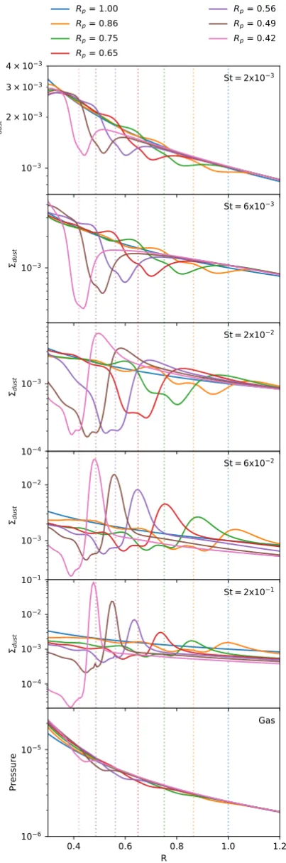
[image:8.595.51.282.256.424.2]Figure 9. Time evolution of the dust density profile for the 30 M⊕migrating planet simulation for particles of various Stokes numbers (top five panels) as well as the time evolution of the pressure profile (bottom panel). The dotted lines show the planet locations. For smaller dust sizes, the dust ring is interior to the planet, while at larger sizes, the dust ring is exterior to it.
Figure 10. Dust velocity (solid line) against disc radius compared to the instantaneous planet velocity (horizontal dotted line) when the planet is at Rp=0.75 for various Stokes numbers. The relative values of the planet velocity compared to the dust velocity (both interior and exterior to the planet) determine whether the dust ring is likely to be prominent interior or exterior to the planet. The locations of the planet and the interior and exterior pressure perturbations are marked with vertical dashed and dotted grey lines, respectively. Note that the oscillations in the inner disc for small Stokes numbers are transient and do not affect the key result.
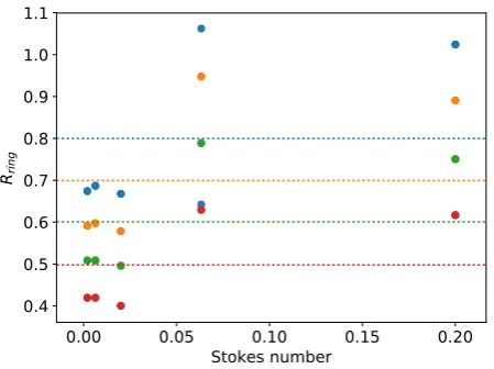
Figure 11. Location of the peak dust density against Stokes number at various times in the simulation of a migrating 30 M⊕planet when the planet is atRp=0.8 (blue), 0.7 (orange), 0.6 (green), and 0.5 (red). The dotted lines show the location of the planet. At small Stokes numbers, the dust peak is interior to the planet and roughly at the same location while at higher Stokes numbers, the peak is exterior to the planet. As the Stokes number (and hence dust size) increases, the location of the peak dust ring sharply moves to larger radial distances. Note that when the planet is atRp=0.8, the dust density interior and exterior to the planet are roughly equal for St=6×10⁻², so two dust rings are evident (as can be seen by the orange and green lines in the fourth panel of Fig.9).
from a dominant inner to a dominant outer ring.5Consequently,
since the wavelength of peak emission depends on the dust size, multiwavelength imaging of the disc mid-plane could in principle indicate planetary migration through a variation of ring morphology with wavelength (i.e. a shift to a more prominent outer ring at longer
wavelengths). This is illustrated in Fig.11which shows how the
location of the dust density maximum varies with Stokes number
(or equivalently, dust size) as the 30 M⊕planet migrates inwards.
In particular, the peak location is roughly independent of Stokes number at small dust sizes, but as the dominant peak shifts from interior to exterior to the planet, a big change in the location of
the dust ring peak will be seen – by as much as a≈50 per cent
change in radial location. As the dust size is increased further, the location of the peak once again varies only a little with dust size. Observing such a rapid change at intermediate dust sizes may well indirectly indicate the presence of a migrating planet. We note that in reality it is not as straightforward as this since grains of various sizes contribute to the flux at any one wavelength. While we expect that the relative intensities of the inner and outer rings should vary with wavelength, it remains to be seen if this shift towards larger grain sizes being concentrated in the outer ring would in practice be detectable via spatially resolved observations of the spectral index in the sub-millimetre (sub-mm) regime (we are investigating this in a separate paper). We note that based on our simulation results, the switch from an inner dominant to an outer dominant dust ring
for a 30 M⊕planet occurs at≈mm sizes at 30 au, assuming silicate
grains (with density 1 g cm−3) in a 0.01M
disc extending out to
100 au, making this result particularly applicable to discs observed by ALMA (see Section 4.3 for a discussion on the transition dust size).
5This signature is distinct from the recent results of Bae, Zhu & Hartmann (2017) where planets produce multiple rings at the same locationsfor all dust sizes, in low viscosity discs.
Furthermore since an interior dust peak is never seen in stationary planet simulations, if a single gap is observed in a disc with a bright inner ring, even at a single wavelength, this is strongly indicative of a migrating planet.
4.2 Planet mass estimates
Rosotti et al. (2016) identified several different ways of
estimat-ing the planet mass from observations. Since they kept the planet fixed on circular orbits, it is important to consider how migration affects their estimates. They showed that quantitative measurements of the planet mass require measuring either the gap width in
scat-tered light images,gap(see their fig. 16 which gives the relation
Mp∝(gap/Rp)3/1.143), or both the position of the bright ring outside
the planet in sub-mm imagesandthe gap width in scattered light
im-ages (see their fig. 17 which gives the relationMp ∝(ring/Rp)1/0.32,
whereringis the distance between the planet and the exterior ring).
We notice that assessing the full impact of planet migration on these criteria would require simulated observations, which we postpone to a future paper; in what follows we simply sketch the possible implications.
Using single wavelength observations and assuming that the ring is exterior to the planet, we can try to understand the errors in the planet mass estimates if one was to use the aforementioned rela-tions derived for stationary planets. In Section 3.1, we show that the position of the pressure maximum is not significantly displaced by migration, which would lead at most to a factor of 2 difference
in planet mass. It has to be noted, however, that Fig.8shows that
in the migrating case there is some shift between the pressure max-imum location and the maxmax-imum in the dust surface density. The effect is minimal for large dust and increases for smaller sizes (see
also Fig.11). As an example, for Stokes numbers of 0.2 and 0.06,
the difference is≈15 per cent, i.e. comparable or slightly smaller
than the shift in the pressure maximum position due to migration,
which would lead to a difference in planet mass of≈50 per cent.
Therefore, to be on the safe side one would need to observe the disc at wavelengths as long as possible in order to use the relations by
Rosotti et al. (2016) to accurately determine the planet mass.
To obtain the gap width from the scattered light observations, the
plots in Fig.1show that the gap shape is affected by migration:
the gap is now asymmetric, and the planet, rather than lying at the centre of the gap, is relatively close to the inner edge of the gap.
For the expression obtained from fig. 17 of Rosotti et al. (2016),
the planet mass is likely to be underestimated as ring will be
underestimated whileRpwill be overestimated. For the expression
obtained from fig. 16 of Rosotti et al. (2016), it is unclear how
this will translate quantitatively to the planet mass criterion without analysing simulated observations. Nevertheless, the fact that the planet is not in the centre of the gap is likely to have the most substantial impact on the mass estimates. Measurements of the planet mass will therefore need to fold in the fact that the planet is migrating.
An error in the planet mass calculation could also occur with the
case we highlight for the 60 M⊕planet, where a secondary bright
ring could be produced close to the planet starting location (see Appendix B). If this maximum is incorrectly used it would lead to a serious overestimate of the planet mass, since the planet has now moved significantly far from it.
On the other hand, if the ring is interior to the planet we cannot
use the relations by Rosotti et al. (2016) to estimate the planet mass.
If there is only a single ring that is interior to a gap then this is a strong indication that planet migration is happening (as stated in
Section 4.1). However if there are multiple rings and gaps in a disc, it may not be so obvious whether the ring is interior or exterior to a planet. One might then obtain not only an incorrect planet mass but also an incorrect planet location.
If a sub-mm ring is suspected to be interior to a planet, further observations at longer wavelengths (dominated by emission from grains with larger Stokes numbers) could be carried out to see if the bright ring then moves exterior to the planet location. The properties of the newly found exterior ring could then be used with
the Rosotti et al. (2016) estimates to determine a planet mass. In this
case, migration can be included in the modelling to aid the accurate determination of the planet mass.
4.3 Threshold size for interior/exterior dust ring
In Section 3.2.2, we show that the external density enhancement can
only occur if|vdust|>>vpl, while for|vdust|vplthe external
dust ring does not form. Therefore, an approximate criterion for the threshold size at which the switch between the dominant inner and
outer rings occurs is|vdust| = |vpl|. Using equation (10), recognizing
that we are concerned with St<1 so that St+St−1∼St−1, and
omitting order unity factors, we find that
vdust≈
H R
2
Stvk
∂logP
∂logR. (11)
Equation (7) can be differentiated to give the planet velocity
vpl∼
Rp
τI
, (12)
where the analytical expression forτI is given by equation (8).
Equating these two velocity terms gives expressions for the thresh-old Stokes number and dust size as
St∼ 2|p|
RppMp
H R −2 1 vk ∂∂loglogPR
−1 (13) and
a∼ |p|
RppMp
ρs H R −2 1 vk ∂logP
∂logR
−1, (14) respectively. Note that since this is essentially a comparison of the planet velocity and the velocity of the dust being supplied to the pressure perturbation external to the planet, the quantities marked with a subscript ‘p’ are evaluated at the planet’s location while all other quantities are evaluated further out in the disc. Using equation (9) and assuming surface mass density and temperature
profiles ofR−1andR−1/2, respectively, as modelled in this paper,
these expressions become
St∼0.03
5 gcm−2
R 30 au
2
Mp
30 M⊕
M M −2 × H /R
0.04
−4
(15)
and
a∼0.7
5 gcm−2
2
R 30 au
2
Mp
30 M⊕
M M −2 × H /R
0.04
−4
ρs
1 gcm−3
−1
mm (16)
whereρsis the internal density of the dust grains. As mentioned
in Section 4.1, this critical grain size at which the ring should switch between interior and exterior to the planet (assuming silicate
grains with density 1 g cm−3 at a radial location of 30 au in a
0.01Mdisc extending out to 100 au with a surface density slope
of ∝ R−1, aspect ratio given byH/R = 0.04(R/R
0)1/4and a
30 M⊕ planet) is a≈mm. Since equation (14) has a quadratic
dependence on the disc surface mass density, a quartic dependence on the disc aspect ratio and a linear dependence on the planet mass, this expression for the threshold dust size is highly dependent on the
disc and planet properties. We evaluate equation (15) for our 30 M⊕
simulation and find that the threshold Stokes number is≈0.022.
This analytically determined expression is in agreement with our
simulations which show a threshold between St=0.02 and 0.06
(Fig.9).
4.4 Caveats
Initial set-up: in our simulations, we migrate the planet as soon as we place it in the disc, while often in planet–disc interaction simulations, planets are held on a fixed circular orbit at the initial location for several orbits before being allowed to migrate. However, we choose not to do this as we do not want the planet to artificially create a pressure trap as a result of this and we want to see that any dust trapping that occurs is real in the presence of a migrating planet. Note that the feature of the calculations that is particularly sensitive to this initial set-up is the extra bump exterior to the planet. However, this only has a significant effect on the dust density distribution in
the case of the 60 M⊕planet.
Planet growth:we also do not grow the planet’s mass over time, while in reality, the planet would grow slowly initially and then undergo runaway accretion. Ideally self-consistent calculations with a planet growing at a realistic rate that starts to migrate as it grows (assuming the growth time-scales are not slow compared to the migration time-scale) are needed to determine the robustness of these results. However, it is important to note that the regime that we explore, i.e. without accretion on to the planet, is still relevant because it has been shown that (i) the critical core mass for runaway
gas accretion can be as much as 60M⊕ (Rafikov2006), and (ii) it
is no longer clear what conditions runaway accretion occurs under
(Ormel, Kuiper & Shi2015; Cimerman, Kuiper & Ormel2017;
Ormel, Shi & Kuiper2015; Lambrechts & Lega2017), and (iii) there
are many rocky super-Earths with only a 5–10 per cent hydrogen envelope (in mass), suggesting that gas accretion is slow (Hadden &
Lithwick2017).
Backreaction:we do not include backreaction of the dust on the gas in these simulations. While this can be potentially important
for dust-to-gas ratios of∼1, for our parameters backreaction only
significantly affects the gas velocity for St>0.1 and thus we do
not expect it to be a major factor (see Appendix D). We point out, though, that in cases where the dust-to-gas ratio becomes large, de-tailed modelling should include this effect, which may be important for interpreting observations.
Dust growth:since the dust growth time-scale is comparable to or shorter than the radial drift time-scale (Birnstiel, Klahr & Ercolano
2012), to complete the picture of dust evolution one should consider
the growth and fragmentation of dust in the simulations.
Migration direction: this study only considers the effect that inward migration has on dust rings when planets migrate at the Type I rate. It is possible that for part of a planet’s radial evolution, it may
migrate in an outward direction (Lyra & Klahr2011; Ayliffe & Bate
2010,2011; Bitsch & Kley2010,2011; Bitsch et al.2013,2014a,
2014b; Paardekooper & Mellema2006,2008) or end up in a zero torque location with no net migration with respect to the rest of
the disc (Lyra & Klahr2011; Bitsch & Kley2011; Bitsch et al.
2013,2014a). If the planet ends up in a zero torque location, we expect that the formation and evolution of dust rings follow what we already know from stationary planet simulations: i.e. that a ring only forms exterior to the planet’s location. In the case of outward migration, we expect the ring to form exterior to the planet for all dust sizes considered, though further studies are needed to address this scenario.
5 C O N C L U S I O N S
We perform 2D hydrodynamical simulations using gas and dust to understand the formation and evolution of dust rings in the presence
of low-mass (12–60 M⊕) migrating planets. We find that the gas
pressure profile is significantly different compared to that in the presence of stationary planets: the pressure perturbation exterior to the planet is weaker while that interior to the planet becomes more important for migrating planets. Dust can therefore be enhanced both interior and exterior to the planet and the result is governed by the relative values of the planet and dust velocities. For small sizes, the dust velocity in the outer disc is too small to keep up with the moving pressure maximum, while in the inner disc, it moves faster and can collect forming a dust density enhancement interior to the planet. On the other hand, for large sizes, the dust velocity in the exterior disc is large enough to keep up with the pressure perturbation (maximum or point of inflection), resulting in a dust density enhancement exterior to the planet. Consequently, the location of the dust ring varies for different dust sizes, varying
by as much as ≈50 per cent. There is also an intermediate size
where the density enhancement is comparable interior and exterior to the planet. The switch between a dominant inner to a dominant exterior bright ring occurs when the velocity of the dust in the outer disc is roughly equivalent to the planet velocity. We predict that the location of the dust ring in the disc mid-plane observed at different wavelengths will shift outwards significantly at a particular wavelength. Therefore in principle, it may be possible to use the location of dust rings in order to detect planetary migration, although the feasibility of this measurement is yet to be established.
AC K N OW L E D G E M E N T S
FM acknowledges support from The Leverhulme Trust, the Isaac Newton Trust, and the Royal Society Dorothy Hodgkin Fellowship. GR, RB, and CC are supported by the DISCSIM project, grant agreement 341137 funded by the European Research Council un-der ERC-2013-ADG. This work was unun-dertaken on the COSMOS Shared Memory system at DAMTP, University of Cambridge oper-ated on behalf of the STFC DiRAC HPC Facility. This equipment is funded by BIS National E-infrastructure capital grant ST/J005673/1 and STFC grants ST/H008586/1 and ST/K00333X/1. This work also used the DiRAC Data Centric system at Durham University, operated by the Institute for Computational Cosmology on behalf
of the STFC DiRAC HPC Facility (www.dirac.ac.uk). This
equip-ment was funded by a BIS National E-infrastructure capital grant ST/K00042X/1, STFC capital grant ST/K00087X/1, DiRAC Oper-ations grant ST/K003267/1, and Durham University. DiRAC is part of the National E-Infrastructure. This research was also supported by the Munich Institute for Astro- and Particle Physics of the DFG cluster of excellence ‘Origin and Structure of the Universe’. This
paper made use ofNUMPY(Travis2006),SCIPY(Jones, Oliphant &
et al. 2001), and MATPLOTIB(Hunter2007). We also thank the
referees for their comments.
R E F E R E N C E S
Alexander R., Pascucci I., Andrews S., Armitage P., Cieza L., 2014, Proto-stars and Planets VI, Univ. Arizona Press, Tucson, AZ, p. 475 Alexander R. D., Armitage P. J., 2009,ApJ, 704, 989
Alibert Y. et al., 2006,A&A, 455, L25 ALMA Partnership et al., 2015,ApJ, 808, L3 Andrews S. M. et al., 2016,ApJ, 820, L40
Ataiee S., Baruteau C., Alibert Y., Benz W., 2018,A&A, 615, A110 Ataiee S., Pinilla P., Zsom A., Dullemond C. P., Dominik C., Ghanbari J.,
2013,A&A, 553, L3
Ayliffe B. A., Bate M. R., 2010,MNRAS, 408, 876 Ayliffe B. A., Bate M. R., 2011,MNRAS, 415, 576 Bae J., Zhu Z., Hartmann L., 2017,ApJ, 850, 201 Baruteau C. et al., 2014, Protostars and Planets VI, 667 Benisty M. et al., 2015,A&A, 578, L6
Ben´ıtez-Llambay P., Masset F. S., 2016,ApJS, 223, 11
Biddle L. I., Johns-Krull C. M., Llama J., Prato L., Skiff B. A., 2018,ApJL, 853, L34
Birnstiel T., Andrews S. M., Pinilla P., Kama M., 2015,ApJ, 813, L14 Birnstiel T., Klahr H., Ercolano B., 2012,A&A, 539, A148
Bitsch B., Crida A., Morbidelli A., Kley W., Dobbs-Dixon I., 2013,A&A, 549, A124
Bitsch B., Kley W., 2010,A&A, 523, A30 Bitsch B., Kley W., 2011,A&A, 536, A77
Bitsch B., Lambrechts M., Johansen A., 2015,A&A, 582, A112
Bitsch B., Morbidelli A., Johansen A., Lega E., Lambrechts M., Crida A., 2018,A&A, 612, A30
Bitsch B., Morbidelli A., Lega E., Crida A., 2014a,A&A, 564, A135 Bitsch B., Morbidelli A., Lega E., Crida A., Kretke K., Crida A., 2014b,
A&A, 570, A75
Chiang E., Laughlin G., 2013,MNRAS, 431, 3444 Ciardi D. R. et al., 2015,ApJ, 809, 42
Cimerman N. P., Kuiper R., Ormel C. W., 2017,MNRAS, 471, 4662 Clarke C. J., et al. 2018,ApJ, 866, L6
Crida A., Morbidelli A., Masset F., 2006,Icarus, 181, 587 David T. J. et al., 2016,Nature, 534, 658
de Val-Borro M., Artymowicz P., D’Angelo G., Peplinski A., 2007,A&A, 471, 1043
de Val-Borro M. et al., 2006,MNRAS, 370, 529 Dipierro G., Laibe G., 2017,MNRAS, 469, 1932 Dipierro G. et al., 2018,MNRAS, 479, 4187 Donati J. F. et al., 2016,Nature, 534, 662 Dong R., Fung J., 2017,ApJ, 835, 38
Dong R., Rafikov R. R., Stone J. M., 2011,ApJ, 741, 57
Duffell P. C., Haiman Z., MacFadyen A. I., D’Orazio D. J., Farris B. D., 2014,ApJ, 792, L10
Dullemond C. P., Penzlin A. B. T., 2018,A&A, 609, A50 D¨urmann C., Kley W., 2015,A&A, 574, A52
D’Angelo G., Lubow S. H., 2010,ApJ, 724, 730 Ercolano B., Rosotti G., 2015,MNRAS, 450, 3008
Ercolano B., Rosotti G. P., Picogna G., Testi L., 2017,MNRAS, 464, L95 Fedele D., et al., 2018,A&A, 610, A24
Fedele D. et al., 2017,A&A, 600, A72 Fressin F. et al., 2013,ApJ, 766, 81
Garaud P., Barri`ere-Fouchet L., Lin D. N. C., 2004,ApJ, 603, 292 Goldreich P., Tremaine S., 1980,ApJ, 241, 425
Gonzalez J.-F., Laibe G., Maddison S. T., 2017, MNRAS, 467, 1984 Hadden S., Lithwick Y., 2017,AJ, 154, 5
Hallam P. D., Paardekooper S.-J., 2017,MNRAS, 469, 3813 Hunter J. D., 2007,Comput. Sci. Eng., 9, 90
Isella A. et al., 2016,Phys. Rev. Lett., 117, 251101 Jacquet E., Gounelle M., Fromang S., 2012,Icarus, 220, 162 Johns-Krull C. M. et al., 2016,ApJ, 826, 206
Jones E., Oliphant T., Peterson P., et al., 2001, SciPy: Open Source Scientific Tools for Python, available at:https://www.scipy.org/citing.html
Juh´asz A., Benisty M., Pohl A., Dullemond C. P., Dominik C., Paardekooper S.-J., 2015,MNRAS, 451, 1147
Kanagawa K. D., Tanaka H., Muto T., Tanigawa T., Takeuchi T., 2015, MNRAS, 448, 994
Kley W., Nelson R. P., 2012, ARA&A, 50, 211 Kratter K., Lodato G., 2016, ARA&A, 54, 271
Lambrechts M., Johansen A., Morbidelli A., 2014,A&A, 572, A35 Lambrechts M., Lega E., 2017,A&A, 606, A146
Lee M. H., Peale S. J., 2002,ApJ, 567, 596
Lin D. N. C., Bodenheimer P., Richardson D. C., 1996,Nature, 380, 606 Lin D. N. C., Papaloizou J., 1986,ApJ, 309, 846
Lissauer J. J. et al., 2011,ApJS, 197, 8 Lithwick Y., Wu Y., 2012,ApJ, 756, L11 Long F., et al., 2018, ApJ
Lyra W., Klahr H., 2011,A&A, 527, A138
Machida M. N., Kokubo E., Inutsuka S.-I., Matsumoto T., 2010, MNRAS, 405, 1227
Malik M., Meru F., Mayer L., Meyer M., 2015,ApJ, 802, 56 Mayor M. et al., 2011, preprint (arXiv)
Montesinos M., Perez S., Casassus S., Marino S., Cuadra J., Christiaens V., 2016,ApJ, 823, L8
Morton T. D., Johnson J. A., 2011,ApJ, 738, 170
Okuzumi S., Momose M., Sirono S.-i., Kobayashi H., Tanaka H., 2016,ApJ, 821, 82
Ormel C. W., Kuiper R., Shi J.-M., 2015,MNRAS, 446, 1026 Ormel C. W., Shi J.-M., Kuiper R., 2015,MNRAS, 447, 3512
Paardekooper S.-J., Baruteau C., Crida A., Kley W., 2010,MNRAS, 401, 1950
Paardekooper S.-J., Baruteau C., Kley W., 2011,MNRAS, 410, 293 Paardekooper S.-J., Mellema G., 2004,A&A, 425, L9
Paardekooper S.-J., Mellema G., 2006,A&A, 459, L17 Paardekooper S.-J., Mellema G., 2008,A&A, 478, 245 Petrovich C., Rafikov R. R., 2012,ApJ, 758, 33
Pinilla P., Flock M., Ovelar M. d. J., Birnstiel T., 2016,A&A, 596, A81 Pinilla P., Pohl A., Stammler S. M., Birnstiel T., 2017,ApJ, 845, 68 Rafikov R. R., 2002,ApJ, 569, 997
Rafikov R. R., 2006,ApJ, 648, 666
Rapson V. A., Kastner J. H., Millar-Blanchaer M. A., Dong R., 2015,ApJ, 815, L26
Rasio F. A., Ford E. B., 1996,Science, 274, 954
Reg´aly Z., Juh´asz A., S´andor Z., Dullemond C. P., 2012,MNRAS, 419, 1701
Rosotti G. P., Booth R. A., Clarke C. J., Teyssandier J., Facchini S., Mustill A. J., 2017,MNRAS, 464, L114
Rosotti G. P., Juhasz A., Booth R. A., Clarke C. J., 2016,MNRAS, 459, 2790
Ruge J. P., Flock M., Wolf S., Dzyurkevich N., Fromang S., Henning T., Klahr H., Meheut H., 2016,A&A, 590, A17
Shakura N. I., Sunyaev R. A., 1973, A&A, 24, 337
Takeuchi T., Miyama S. M., Lin D. N. C., 1996,ApJ, 460, 832 Travis E. O., 2006, A Guide to NumPy. Trelgol Publishing, USA van der Marel N. et al., 2013,Science, 340, 1199
van der Plas G. et al., 2017,A&A, 597, A32 van Eyken J. C. et al., 2012,ApJ, 755, 42
Wagner K., Apai D., Kasper M., Robberto M., 2015,ApJ, 813, L2 Walsh K. J., Morbidelli A., Raymond S. N., O’Brien D. P., Mandell A. M.,
2011,Nature, 475, 206
Zhu Z., Stone J. M., Rafikov R. R., Bai X.-n., 2014,ApJ, 785, 122
A P P E N D I X A : T OY M O D E L F O R T H E O U T E R G A S B U M P C AU S E D B Y H I G H - M A S S P L A N E T S
Here, we investigate the origin of the second pressure maximum, which appears just outside the initial location of the highest mass
planet (Fig.4) with a toy model designed to qualitatively explain
the behaviours seen in the simulations. We consider the influence of the torques exerted by the planet on the disc modelled in the framework of a 1D viscous evolution model.
We assume that the angular momentum evolution of the disc driven by the planet can be modelled locally, and with a torque profile that is not too different to the linear one acting on the planet. For the torque density profile, we use
(R, Rp)=f()2pR 2 pq 2 Rp Hp 4 , (A1)
whereqis the planet-to-star mass ratio,=(R−Rp)/0.9Hp, and
f()=0.075
exp
−(−0.2)2 2
−exp
−(+0.2)2 2
.
(A2)
Quantities with a subscript ‘p’ are evaluated at the location of the planet. This profile has a similar shape to the torque density exerted
by the disc on the planet found by D’Angelo & Lubow (2010), but
the factor 0.075 results in an amplitude that is about a factor of two smaller. Assuming that the gas remains on circular orbits and neglecting viscosity, the torque gives rise to a radial velocity of the gas,
vr=
2(R, Rp)
R . (A3)
In the toy model, we takeH/R=0.05 and the planet mass to be
60 M⊕.
The top panel of Fig.A1shows the evolution of radius of
differ-ent fluid elemdiffer-ents under this torque, assuming the planet migrates according to equation (7) with a migration time-scale of 327 orbits, and the middle panel shows the resulting surface density. This shows that torques from the planet naturally create both the gap near the planet and the secondary maximum outside of the planet’s initial location. The upper panel demonstrates why the interior maximum and secondary maximum external to the planet form: most fluid el-ements that are initially inside the planet’s location (highlighted in blue) experience a net inward migration. This is because they either only move inwards, or first undergo an inward migration until the planet catches up with them then undergo an outward migration after the planet has passed. However, those elements that start very close and interior to the planet location or just outside it only un-dergo a net outward migration (highlighted in red), resulting in a large net outward motion. Since those fluid elements that are ini-tially located far outside the location of the planet hardly move at all, this inevitably leads to the formation of an additional bump in the density exterior to the planet. This effect is not seen for lower
mass planets simply because it is weaker: the torque depends onq2,
while the Type I migration time-scale is ∝ q−1, resulting in the net
motion of the gas scaling asq. Similarly, the gap depth in the toy
model increases as the planet migrates because the migration time
of thegasscales asR/vr∝−p1, while we have taken the migration
time-scale of the planet to be fixed. Thus, the net motion of the gas is relatively larger at smaller radii.
Finally, in the bottom two panels, we show the surface density with the effects of viscosity included. To do this, we solve the viscous evolution equation with the addition of the torque from the planet:
∂
∂t = 1 R
∂ ∂R
3R1/2 ∂
∂R(νR
1/2
)−2(R, Rp)−1
, (A4)
takingν=αvisccsHandαvisc=10−3. This shows that the addition of
viscosity causes the secondary maximum to spread and weaken over time, and also reduces the depth of the primary planet induced gap. Note that the absence of the extra structure in the gas density close to the planet in the toy model is evidence that the shape of the real