First passage and first hitting times of Lévy flights and Lévy walks

PAPER

First passage and

fi

rst hitting times of Lévy

fl

ights and Lévy walks

Vladimir V Palyulin1 _{, George Blackburn}2,3_{, Michael A Lomholt}4_{, Nicholas W Watkins}3,5,6,7_,

Ralf Metzler5 _{, Rainer Klages}2,8,9 _{and Aleksei V Chechkin}5,10

1 _{Centre for Computational and Data-Intensive Science and Engineering, Skolkovo Institute of Science and Technology, Nobelya Ulitsa 3,} Moscow, 121205, Russia

2 _{Max Planck Institute for the Physics of Complex Systems, Nöthnitzer Straße 38, D-01187, Dresden, Germany} 3 _{Centre for Fusion, Space and Astrophysics, University of Warwick, Coventry, United Kingdom}

4 _{MEMPHYS—Centre for Biomembrane Physics, Department of Physics, Chemistry, and Pharmacy, University of Southern Denmark,} DK-5230, Odense M, Denmark

5 _{Institute for Physics & Astronomy, University of Potsdam, D-14476 Potsdam-Golm, Germany}

6 _{Centre for the Analysis of Time Series, London School of Economics and Political Sciences, London, United Kingdom} 7 _{Faculty of Science, Technology, Engineering and Mathematics, Open University, Milton Keynes, United Kingdom} 8 _{Institut für Theoretische Physik, Technische Universität Berlin, Hardenbergstraße 36, D-10623, Berlin, Germany} 9 _{Queen Mary University of London, School of Mathematical Sciences, Mile End Road, London E1 4NS, United Kingdom}

10 _{Akhiezer Institute for Theoretical Physics National Science Centre‘Kharkov Institute of Physics and Technology’, Kharkov 61108,} Ukraine

E-mail:[email protected]

Keywords:Lévyflights, Lévy walks,first-passage time,first-hitting time

Abstract

For both Lévy

fl

ight and Lévy walk search processes we analyse the full distribution of

fi

rst-passage and

fi

rst-hitting

(or

fi

rst-arrival)

times. These are, respectively, the times when the particle moves across a

point at some given distance from its initial position for the

fi

rst time, or when it lands at a given point

for the

fi

rst time. For Lévy motions with their propensity for long relocation events and thus the

possibility to jump across a given point in space without actually hitting it

(‘leapovers’), these two

de

fi

nitions lead to signi

fi

cantly different results. We study the

fi

rst-passage and

fi

rst-hitting time

distributions as functions of the Lévy stable index, highlighting the different behaviour for the cases

when the

fi

rst absolute moment of the jump length distribution is

fi

nite or in

fi

nite. In particular we

examine the limits of short and long times. Our results will

fi

nd their application in the mathematical

modelling of random search processes as well as computer algorithms.

1. Introduction

When a stochastic processx(t)first reaches a given threshold value in many scenarios follow-up events are triggered: shares are sold when their value crosses a pre-set target amount, or chemical reactions occur when two reactive particles encounter each other in space. The timetat which this triggering eventfirst occurs, is either called thefirst-hitting(first-arrival)or thefirst-passage time, as defined below[1–3]. While the physical analysis offirst-passage time problems has a long history, notably the seminal works by Smoluchowski[4]as well as Collins and Kimball[5], even for the long-studied case of standard Brownian motion[6]significant progress has been achieved within the last decade[2,7–9]. In particular, forfinite domains interesting results were unveiled for the mean and global meanfirst passage times and their geometry-control[7,10]. The often minute particle concentrations inside biological cells and the related concept of the few-encounter limit[11–13]motivated studies to obtain the full probability density function(PDF)offirst-passage times in generic geometries, demonstrating strong defocusing(large spread offirst-passage times)and an intricate interplay between geometry- and reaction-control[13,14].

For non-Brownian stochastic processes additional complications in the determination offirst-passage and

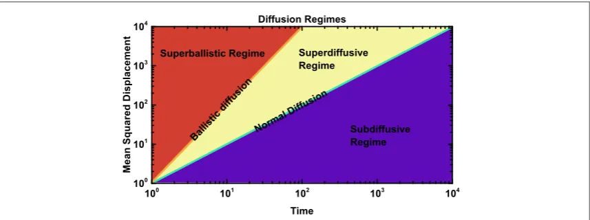
first-hitting times arise. Conceptually, suchanomalous diffusion processesare distinguished according to the value of the anomalous diffusion exponentνin the long time limit of their mean squared displacement(MSD)

x t2

_ò

á ( )ñ = ( )  n n, defined as ensemble average ofx2over the particle PDFP(x,t)[15–20]: the OPEN ACCESS

RECEIVED

26 April 2019

REVISED

23 August 2019

ACCEPTED FOR PUBLICATION

5 September 2019

PUBLISHED

11 October 2019

Original content from this work may be used under the terms of theCreative Commons Attribution 3.0 licence.

Any further distribution of this work must maintain attribution to the author(s)and the title of the work, journal citation and DOI.

range 0<ν<1 corresponds tosubdiffusion(or dispersive transport), while 1<ν<2 is referred to as

superdiffusion(or enhanced transport). Beyond the regimeν=2 of ballistic transport, we encounter

superballistic motion. Sometimes the range 3<ν<5 is calledhyperdiffusion[21]. Examples for anomalous diffusion processes include turbulentflows[22], charge carrier transport in amorphous semiconductors[23], human travel[24], light waves in glassy material[25], biological cell migration[26–29], or transport of

submicron tracer particles andfluorescently labelled molecules inside biological cells and their membranes[18, 30–32]. Figure1shows a schematic representation of the various regimes.

In anomalous diffusion the mentioned complications may arise due to long-ranged correlations, for instance, in the increments of Mandelbrot’s fractional Brownian motion[33], whose strongly non-Markovian character precludes the application of standard analytic methods to determine thefirst-passage dynamics[34–36]. Non-standardfirst-passage andfirst-hitting properties also arise forLévyflight (LF) and Lévy walk (LW)processes, that are in the focus of this study. LWs and LFs are among the most prominent models for the description of superdiffusive processes[15–17,20,37–39]. Both models represent special cases of continuous time random walks[3,40], in which relocation lengths are drawn from a long-tailed Lévy stable distribution with diverging variance. The difference between them is that LFs are Markovian processes in which jumps occur at typical time intervals. Therefore, the resulting LF process is characterised by a diverging MSD_áx t2_{( )ñ[3,15,40,41]. LWs, in contrast, include a}

spatiotemporal coupling between jump lengths and waiting times, penalising long jumps with long waiting times, effectively introducing afinite velocity[42]. Jump lengths and waiting times may be coupled linearly, such that the resulting LW moves in a given direction with a constant speed until velocity reversal after a given waiting time, the velocity model[43], or the space-time coupling may have a power-law type[40]. The velocity may also be considered to change from one step to another[44,45]. Interestingly, for certain parameters even Lévy walks have an infinite variance, namely, when there is a distribution of velocities associated with different path lengths[45]. LFs and LWs are non-ergodic in the sense that long time and ensemble averages of physical observables are different[19,20,45–49]. The linear response behaviour and time-averaged Einstein relation of LWs have been studied, as well[50,51]. We note that LFs and LWs have also been formulated in heterogeneous environments[52,53].

While for Brownian motion the events offirst-passage andfirst-hitting(orfirst-arrival)are identical because space is being explored continuously[54], the possibility of long, non-local jumps lead to‘leapovers’[55,56], single jumps in which a given point is overshot by some leapover length, as illustrated infigure2: for random walk processes with diverging variance of the jump length PDF, the event offirst-passage becomes

fundamentally different from that offirst-hitting, and it is intuitively clear thatfirst-hitting a target is harder

(less likely)than thefirst-passage.

LFs and LWs have been studied for considerable time, however, the systematic comparison of some of their

first passage properties started only recently[57]. We here systematically investigate thefirst-passage andfi rst-hitting properties of LFs and LWs in one dimension by drawing generic conclusions on their differences and similarities. This is an importantfirst step in the assessment of these two fundamental random search processes. Further applications of non-local, Lévy-type search are found in computer algorithms such as simulated annealing[58]. In higher dimensions the comparison is more complicated due to various possible definitions of LWs and LFs[59,60]. In particular, so far studies of LFs and LWs mostly focused on the long-time features. However, in all search processes the short-time properties do contribute to the efficiency of the search[61], and

For normal diffusion the MSD grows linearly with time. However, other types of‘anomalous diffusion’are widely observed, for which the MSD grows as_áx t2_{( )ñ}tn_{, where the anomalous diffusion exponentνdiffers from unity.‘Subdiffusion’is slower than normal} diffusion, corresponding toν<1. Faster diffusion splits into the regimes of‘superdiffusion’with 1<ν<2,‘ballistic motion’with

in the light of the aforementioned scenarios of the few-encounter limit become even more relevant. We therefore pay considerable attention to the characteristics of the short-timefirst-passage andfirst-hitting properties of LFs and LWs.

Our paper is organised as follows. In section2we briefly review the rôle of LFs and LWs in random search processes, followed by setting thefirst-passage andfirst-hitting scenarios in section3. Section4reports thefi rst-passage properties of LFs and LWs, thefirst-hitting properties of both processes are then investigated in section5. A summary and discussion is provided in section6, and details of the mathematical derivations are deferred to the appendices.

2. The role of L

é

vy

fl

ights and walks in random target search

The term LF was coined by Benoît Mandelbrot in honour of his advisor, the French mathematician Paul Lévy, at École Polytechnique in Paris. In his famed treatise on the fractality of nature[62], Mandelbrot studied random walk processes with scale-free jump length distributions, leading to fractal trajectories of clusters of local motion interspersed with long relocations, on all scales.

As mentioned above LFs are Markovian and possess a diverging MSD. In that sense they are in most cases

‘unphysical’, as they appear to possess an infinite speed. While spatiotemporally coupled LWs provide a‘ non-pathological’description withfinite speed, LFs do have their justification in the following senses:first, when the process involves long-tailed jump lengths in some‘chemical’co-ordinate but local jumps in the physical, embedding space, the argument about a diverging MSD does not hold. An example is the random search of proteins on a DNA chain that is represented as a fast-folding chain in three dimensions[63]. Second, when we solely speak about the spatial trajectory described by the searcher yet are oblivious of the corresponding time trace, it is legitimate to speak of LFs. Third, the observed motion may be considered scale-free only within a limited range of relocation lengths, beyond which cutoffs may exist[64–66]. Fourth, we note that only very rarely have experimental foraging studies really tested for LWs[20,67]. Fifth, in some physical systems the measured data indicate a divergence of the kinetic energy[68]. Finally, LWs represent a much harder

mathematical problem than LFs while the LF assumption may already provide valuable insight into the system. For these reasons we study LFs and LWs in parallel, and we point out their commonalities and differences.

Interest in both LF and LW models in physics arose in the context of simple one-dimensional deterministic maps that generate superdiffusive motion encountered within the context of phase diffusion in Josephson junctions[69,70]. It was then shown that diffusion in these maps could be understood in terms of LWs[43, 69–71]. Further motivation to investigate LFs and LWs was sparked by a remark of Michael Shlesinger and Joseph Klafter, that scale-free motion may present a more efficient means for exploring space in one and two dimensions as compared to Brownian motion[72]. The argument goes that while Brownian dynamics features repeated returns to already explored regions causing oversampling[3,63], scale-free LFs and LWs, in contrast, avoid these returns and, hence, yield a more efficient search strategy11.

Figure 2.Illustration of the difference between an event offirst-passage(top), when the walker crosses a target atx=0 in a single jump event and overshoots it by the leapover length[56], and an event offirst-hitting(first-arrival, bottom)at the target. The initial position of the walker isx=x0.

11_{Note that many search processes indeed run off in effectively two dimensions}

LFs and LWs[42,61,78,82–86]. Generally, most of the intermittent and multimodal search strategies can be described as a combination of a local exploration mode and a scale-free(long relocation)mode[78,87], where the frequent, long, relocations are described by Lévy motions[61,82].

Interestingly, there exists a direct connection between the biological strategy of random search for targets and the mathematical problem offirst-passage andfirst-hitting. In foraging theory one distinguishes between cruise and saltatory foragers. While in cruise search the forager looks out for targets during the movements, the forager is blind for its targets when moving for saltatory search, for which the searcher needs to land exactly on

(or very close to)the target to actually detect it[80,88]. A cruise forager searching for a single target, however, is modelled mathematically as afirst-passage problem while saltatory search for a single target corresponds to a

first-hitting problem. Solving these mathematical problems thus sheds light, at least in more simple, abstract settings, on specific aspects of biological foraging.

As a general rulefirst-hitting problems appear in most target search problems whilefirst-passage relates to the crossing of thresholds. The latter problem has been studied for many decades in the context of Markovian processes

(see, for instance[89])and much initial work related to the Gaussian case. Classic applications offirst-passage include vibration[90], sea states, and earthquakes[91]. Thefirst-passage problem also appears in calculating the time to activation in cases like Gerstein’s and Mandelbrot’s model of neurons[92], and resonant activation[93]. Further motivation comes from applications of the area swept out by Brownian motion up to itsfirst passage, where results can be heuristically motivated fromfirst-passage theory scaling results[94]. Recent interest has included transitions from the bull-to-the-bear market infinance, extreme value statistics of temperature records[95], or the diffusion of atoms in a one-dimensional periodic potential[96]as well as problems of escaping an enemy territory. The existence of heavy-tailed log-pricefluctuations infinance, modelled usingα-stable processes in[97]has indeed been a strong initial motivation for the LFfirst passage problem.

3. Setup of the system: determining

fi

rst-passage and

fi

rst-hitting times

The problem offirst-passage consists in the determination of boundary crossing dynamics of a searcher. In the general casefirst-passage properties can be studied for any kind of domains[1,2,10,13,14]. In this paper we consider the classical 1D setting. We are interested in the event when a searcher crosses the origin for thefirst time after initially being released at positionx0>0(figure2, upper part). For LFs thefirst-passage time corresponds to the moment in time when the searcherfirst hits a coordinate on the negative semi-axis. For LWs thefirst-passage time is defined as the time needed for a particle to reach the origin, that is, only the fraction of the last relocation event(from the arrival point of the previous relocation to crossing the origin)is included in the computation.

Afirst-hitting event occurs when the end point of a jump arrives exactly at the origin. In physics literature the

first-hitting is often also called thefirst arrival[80,98]. Here we will use the term hitting throughout the text to avoid possible ambiguities. Similar to thefirst-passage the event offirst-hitting may be defined for a domain of any shape. Here we concentrate on point-like targets. Thus, in the case of LFs thefirst-hitting corresponds to an exact landing at the target coordinate. For LWs in our 1D scenario an event offirst-hitting occurs when the last relocation ends at the target, that is, in the LW case this corresponds to a searcher who cannot identify the target while crossing it during the relocation event.

Our results are either derived from the fractional Fokker–Planck equation[15,41,52]or are obtained from simulations of the discrete Langevin equation

for the searcher’s positionxn, whereξα(n)is a set of random variables sampled from a symmetric Lévy stable

distribution with the characteristic functionexp( ∣ ∣ )-ka . The time step is chosen asδt=0.001 for LFs in all cases but those which required higher time resolution. In that caseδt=0.0001 was used(figure10). While we keep the generalised diffusion coefficientK_αof dimensioncma sin our analytical results, we set it to unity in the numerical analyses. The noisex_a( )n was computed following the method described in[100]. For LFs the time dependence is then simply obtained by adding the time stepδtto a counter at each jump. The set of landing points for LFs exactly corresponds to the set of end-of-relocation points for LWs and, hence, the same simulation procedure was used for both processes. For LWs, in turn, the parameterδtis not related to the time resolution any longer, but rather describes the width of the jump length distribution. We thus useKadt=0.001for the

first passage of LWs andKadt =0.0005for thefirst hitting problem. In order to compute the time-dependent characteristics for LWs the durations of relocations were calculated from a given relocation length via the speed

v0of the walk that we take as a constant value. In our simulation of LWs the direction at the beginning of each

relocation event is changed with likelihood1

2(that is, the searcher continues in the same direction with

probability1

2), as the jump lengths are taken from the symmetric distribution of theξαentries.

In all cases considered in this paper a searcher eventually crosses the boundary orfinds the target with unit probability. Hence, thefirst-passage andfirst-hitting properties can be characterised by the properly normalised PDFs. We will denote them asÃPF( )t andÃPW( )t for thefirst-passage of LFs and LWs, respectively, andÃHF( )t

andÃHW( )t for thefirst-hitting of LFs and LWs.

4. First-passage properties of L

é

vy

fl

ights and L

é

vy walks

In this section we focus on thefirst-passage dynamics of LFs and LWs. First we analyse the case of LFs. In the following subsection for LWs we compare the results with the LF case.

4.1. First-passage for Lévyflights

Thefirst-passage of LFs, due to their Markovian character and the symmetric jump length distribution is necessarily characterised by the Sparre Andersen-scaling[1,98]in the long time limit. The analytical expression for this limiting behaviour reads[56]12

t x

K 2 t , 2

PF 0

2

3 2

a p a

à ~

G a

a

-( )

( ) ( )

in terms of the initial positionx0and the stable indexαof the jump length PDF. Here and in the following, the

symbol∼denotes asymptotic equality,;means asymptotically equal up to a prefactor(scaling equality), and

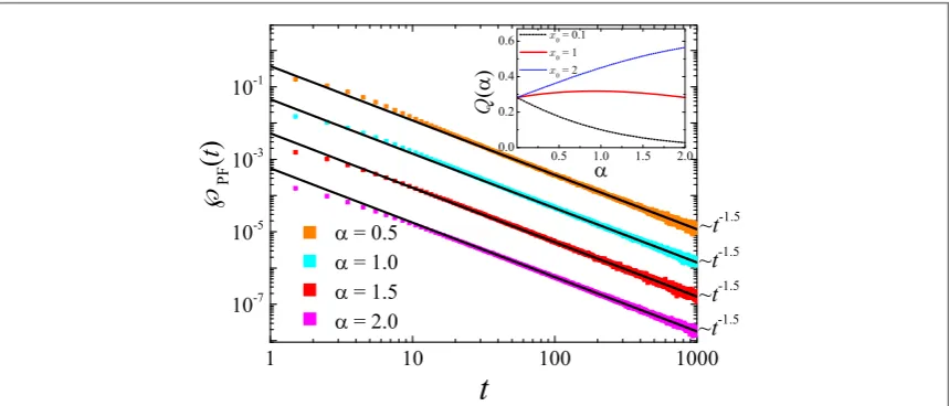
≈means approximately equal. Figure3illustrates that the simulations results(coloured squares)are in perfect agreement with the Sparre Andersen-scaling(2)shown by the black lines forαvalues that are smaller and larger than unity. Note the shift by constant factors between the different results.

Considering the corresponding short time behaviour infigure4one immediately realises that only for the case of Brownian motion(α=2)the PDF increases smoothly with time from the value zero att=0. For LFs withα<2 thefirst-hitting PDF exhibits a non-zero value att=0. For smallαvalues(see the curve forα=0.5 infigure4)the PDF decreases monotonically with time, while for largerαvalues an initial increase is observed, leading to a maximum beyond which the PDF crosses over to the long time Sparre Andersen-scaling. LFs with smallerαvalues have a higher propensity for long jumps, while forα→2 the behaviour converges to the known Lévy–Smirnov law for Brownian motion. The abrupt increase ofÃ( )t att=0 thus stems from LFs that directly overshoot the origin with theirfirst jump away from their initial positionx0. The associated probability

pjumpcan be estimated from the survival probability of the searcher(for the full derivation see appendixA),

p K

x

sin 2

. 3

jump

0

pa a p

» a G

a

( ) ( )

( )

For theαvalues considered infigure4we obtain the concrete values

p

0.178,

0.064, 1

0.017 8,

, 4

K x

K x K

x

jump 2

1 2

2 2

3 2

1 2

0

1 0

3 2

03

a

a

a

»

» =

» =

» =

p

p

p

⎧

⎨ ⎪ ⎪

⎩ ⎪ ⎪

( )

where we usedx0=5 andK_α=1. These values are in perfect agreement with the simulations data infigure4.

12

Analytically one can also obtain the derivative of the PDFÃPF( )t for LFs in the short time limit(appendixA).

It turns out that the monotonic decrease for smallαvalues changes to the initial increase of the PDF at the value

α=2/3, seefigure4. We note that in[101]the‘limited space displacement’of the trajectory corresponding to the Cauchy-Lorentz distribution for relatively low noise intensities at short times was discovered and analysed.

4.2. First-passage for Lévy walks

As laid out before, LWs spatiotemporally couple each relocation distancexwith a time costt=x/v0.

Nevertheless, starting from a Lévy stable jump length distribution, the points of visitation of an LW are identical with those of an LF with the same entries for the sequence of jumps—only the time counter for reaching the points of visitation differs for both processes. Hence, many properties of LWs can be understood from a subordination approach[102]: In some sense, to be specified below, an LW process can be considered as an LF with transformed durations of individual jumps. The PDF for the relocation times for LWs follows from the jump length PDF of LFs, as we show in appendixB. From the point of view of subordination one has to

Figure 3.PDFs offirst-passage times for LFs illustrating the universal Sparre Anderson-scaling(2)valid in the long time limit. Results for four different stable indices_αare shown, as indicated in the graph. Simulations data₍coloured squares₎were obtained from

N=107runs with initial position of the searchersx0=2 and the generalised diffusion coefficientKα=1. Black lines are obtained from equation(2). Note that for the better visual comparison of the PDFs to the exact asymptotic scaling, their values are divided by a factor of 10 forα=1, of 100 forα=1.5, and of 1000 forα=2. The inset shows the behaviour of the prefactor of the long-time dependence;t−3/2,Q( )a =x0a 2 [a pKaG(a 2)]from equation(2), for differentx0and withKα=1. Largerαvalues lead to more pronounced differences in the values ofQ(α).

Figure 4.Short time behaviour of thefirst-passage time PDF for LFs, demonstrating that the change of the slope att=0 occurs for

α=2/3(for which we observe a horizontal tangent). Herepjumpis the probability that the boundary is immediately crossed with the first jump. Number of runs:N=107_{, initial position:x}

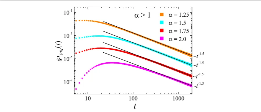
discriminate the two casesα>1 andα„1. Namely, forα>1 the average duration of a jump isfinite, and thus in the limit of a large number of jumps the time characteristics of LWs and LFs will only differ by a prefactor but should have the same scaling in time. From this scaling argument we expect the Sparre Andersen-scaling

t t , 1 5

PW 3 2 a

à _{( )} - / > _{( )}

to hold for the PDFÃPW( )t of thefirst-passage of LWs, as long as 1<α„2. Indeed, the simulations results

presented infigure5for 4 different values ofαnicely corroborate the Sparre Andersen -3

2scaling(5).

The problem of escape of LFs and LWs forα>1 was studied in[57]. The latter paper also proposes a formula for the effective diffusion coefficient for LWs expressed through the LW speedv0, the scaling factorσ0or

the Lévy stable jump length PDF, and the stable indexα(equation(55)in[57]). We derive this formula exactly in appendicesBandC. Having an expression for the effective diffusion coefficientKaLWof LWs it seems pertinent to apply expression(2)to the LW dynamics. However, the numerical values obtained in this vein do not coincide with the simulation results. The values from the analytical results underestimate the simulations data in the limit of longt. This discrepancy is caused by the differences in theshort-time behaviourbetween LFs and LWs. Namely, until the front of an LW reaches the boundary, the PDF offirst-passage has a strictly zero value, due to thefinite propagation front of LWs[20]. Modelling LWs by a rescaled LF process obviously neglects this important short-time feature. Hence a model LF process will exceed the real LW PDF at short short-times and, for reasons of

normalisation, underestimate the PDFÃPW( )t at long times.

For LWs withα„1 the observed long-time scaling deviates from the Sparre Andersen-scaling, as evidenced by the simulations data shown infigure6. Thefitted scaling exponents are consistent with the long time scaling

t t , 1 6

PW 2 1 a

à _{( )} -a - _{( )}

considered in[103]which can also be rationalised in subordination terms. Indeed, the survival probability of an LF in the case of afirst-passage scenario is inversely proportional to the square root of the numbernofflights, that is,SLF( )n n-1 2. Forα<1 the number of jumps scales likenta, such thatSLF( )t ~t-a 2. This

scaling is equivalent to that obtained from the subdiffusive fractional diffusion equation[104]. Since thefi rst-passage time PDF is the negative of thefirst derivative of the survival probability, we getÃPW( )t t-a 2 1-. A

strict derivation of this exponent for LWs can be found in[105], where the general result forÃPW( )s is shown to

be a function of the step length distribution in Laplace space. This general expression produces both the Sparre Andersen-scaling forα>1 and the exponent−1−α/2 forα<1.

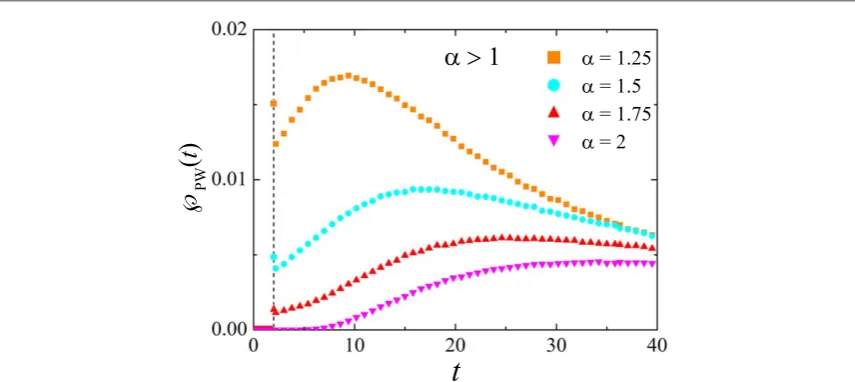
The short-time limit of thefirst-passage time PDFs of LWs shown infigures7and8is noticeably different from the behaviour of LFs(comparefigure4). Namely, for LWs the spatial spreading is limited by a front which travels with the constant speedv0, while for the LF case the PDFÃPF( )t has non-zero values at any non-zero time.

Before the front of an LW reaches the origin the PDF offirst-passage times is identically zero. At exactly

t=x0/v0we observe a jump in the value of thefirst-passage PDF. This jump corresponds to all those walkers

which did not change the direction even once since the process started. Then, similarly to LFs, the function decays monotonically for smallαor has an intermediate maximum.

We notice that in the limitα=2 of Gaussian relocations the resulting motion performed with a constant speed is similar to the model of immortal creepers[106]. For this type of motion thefirst-passage behaviour was

Figure 5.Long time scaling behaviour of thefirst-passage PDFÃPW( )t of LWs for differentα>1. All curves nicely follow the predicted Sparre Andersen-scaling(5). Number of runs:N=107_{, with initial positionx}

0=2. Speed of the LW:v0=1. Note that for the better visual comparison of the PDFs their values are divided by factors of 10 forα=1.5, of 100 forα=1.75 and of 1000 for

studied. However, in the model considered in[106]the creepers change direction with a waiting time PDF

t e t

creeper

y _{( )}=w -w_{, whereωis the characteristic turning frequency. In our case one has to compute the} distribution of relocation times from the Gaussian characteristic function of the process. Forα=2 in our case

(compare appendixB),

v v

v

1

exp

4 ,

2

. 7

0 0

02 2 0 2

0 0

y t

p s

t s t

s p

= ⎛- á ñ =

⎝

⎜ ⎞

⎠ ⎟

( ) ( )

Hence the equation(56)for the survival probability derived in[106]is not directly applicable in our case. Generally, the jump ofÃPW( )t occurs at the very moment when the propagation front, the fraction of

particles having moved the distancevtwithout direction changes, passes through the boundary. This front corresponds to a delta peak with decreasing amplitude, moving with the wave variable∣ ∣x v t0 (appendixD).

Formally, that is, the value of the PDF at the time when this peak reaches the boundary is infinite,

t x v PW 0 0 0

à ( = ) ¥, as the survival probability changes as a step function13. In the simulations the PDF

values are obtained from collecting crossing events infinite bins whose size represents the time resolution. Hence, thefinite numerical values att0are an artefact of the binning, and afiner mesh will produce larger values

Figure 6.Long time scaling of thefirst-passage PDFÃPW( )t of LWs for differentα„1. Thefitted scaling exponents are in nice agreement with the prediction of equation₍6₎. The results are obtained fromN_=107_{runs with initial positionx}

0=2, and relocation speedv0=1. Note that for the better visual comparison of the PDFs their values are divided by a factor of 10 forα=0.5, of 100 for

α=0.75 and of 1000 for_α=1.

Figure 7.Short-time behaviour of thefirst-passage PDF of LWs for differentα„1. The results are averaged overN=107_{runs with} initial position wasx0=2 and LW speedv0=1.

13

ofÃPW( )t (att=2 for the simulations parameters used forfigure8). We verified that this is indeed the case, as

demonstrated by table1.

The difference in behaviour of thefirst-passage PDF between the casesα„1 andα>1 as shown in

figures7and8can be explained by the difference in the shape of the LW propagators(comparefigureH1). In fact, forα>1 the position PDF of LWs has a front(smaller spikes infigureH1)producing the jump in thefi rst-passage PDF, then the main, bell-shaped part of the PDF arrives, and thefirst-passage PDF grows gradually. For

α<1, in contrast, the fronts are the only maxima in the position PDF, and thus the PDF offirst-passage has a non-zero value and then decays monotonically.

5. First-hitting properties of L

é

vy

fl

ights and L

é

vy walks

In order to observefirst-hitting events in a one-dimensional setting, we necessarily need to require that thefirst absolute momentá ñ∣ ∣x of the jump length PDF exists, corresponding to the requirementα>1[61,81]. For the opposite case of 0<α<1 the associatedfirst-hitting time PDF vanished identically to zero. We do not consider the latter case here. For LWs an event offirst-hitting in our setting occurs when the end point of a relocation with speedv0hits the target.

5.1. First-hitting properties of Lévyflights withα>1

The probability offirst-hitting(seefigure2)clearly depends on the exact target size[107]. Here we will

concentrate on the case of point-like targets. Detailed studies of thefirst-hitting properties of LFs were presented in[80,81,98]. Analytical derivations are based on the fractional Fokker–Planck equation[15,52]with a sink term,

f x t

t K

f x t

x t x

, ,

, 8

HF d

¶

¶ =

¶

¶ - Ã

a a

a

( ) ( )

∣ ∣ ( ) ( ) ( )

where the fractional derivative is defined in terms of its Fourier transform,

ò

-¥ ¥

( )[ ( ) ∣ ∣ ]

k f k t,

-_{∣ ∣}a _{( ), wheref(k,t)is the Fourier transform off(x,t). Equation(8)can be easily modified to include an}

Figure 8.Short-time behaviour of thefirst-passage PDF of LWs for differentα>1. The results are averaged overN=107runs, the initial position wasx0=2, and the LW speed isv0=1. The bin size was chosen as 0.1.

Table 1.Values of the LWfirst passageÃPW( )t att=2 for two differentαvalues and different bin sizes.

external drift[81], to the case of multiple point-like targets[82], or to include an additional Brownian or Lévy component with different stable indexa¢[61,82]. We consider here a perfectly absorbing sink. The case of a

finite absorption strength can be found in[108]. Equation(8)can be solved in Laplace space for the initial conditionf x( , 0)=d(x-x0)[98], yielding

s

k k

d

d . 9

s K k

s K k

HF

e 1

kx

i 0

ò

ò

à = -¥

¥ +

-¥ ¥

+

a a

a a

( ) ∣ ∣ ( )

∣ ∣

From inverse Laplace transform of this expression we obtain a new result for thefirst-hitting time PDF in time

(see appendixE),

t sin K t d cosk kx E K k t , 10

HF

1

1 1

0 0 1,1

ò

a p a p

à = a a a

-a a a

- ¥

( ) ( ) ( ) ( ) ( )

whereE1,1 a(-K k ta a)is a two-parameter Mittag-Leffler function, which can be defined by its series expansions [109]

Figure 9.First-hitting time PDF for LFs with different_αillustrating the long time scaling law₍12₎, here represented by the black lines with slopes predicted by the analytical expression. The coloured symbols depict the simulations results. Note that for better visual comparison the PDFs are divided by a factor of 10 forα=1.5, of 100 forα=1.75, and of 1000 forα=2. We choseKα=1.

E z z

k z k z

1

, 0 11

k

k

k

k

k

,

0 1

1

å

å

- =

-G + ~

-G - >

a b

= ¥

=

¥ +

( ) ( )

( )

( )

( ) ( )

around zero and infinity, respectively. From the latter expansion we immediately recover the well-established power law asymptotic for thefirst-hitting time PDF of LFs[98],

t t 12

HF 1 2

à _{( )} a- _{( )}

at long times(compare equation(E.7)and its derivation in appendixE). We here also derive the short time scaling law

t t 13

HF 1

à _{( )} a _{( )}

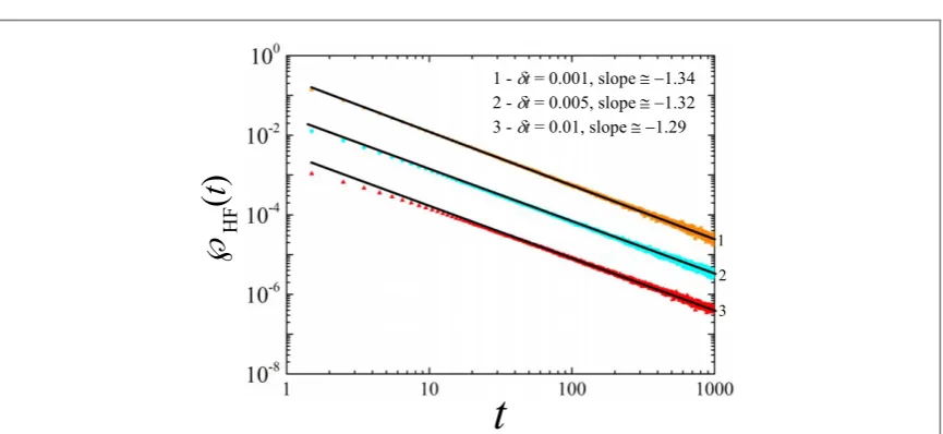
in appendixF. The full expression(10)can be evaluated numerically to plot the analytical solution of(8). To determine thefirst-hitting time PDF from simulations of a searcher jumping according to a Lévy stable jump length distribution, we need to endow the target with afinite sized. This size needs to be large enough to guarantee sufficiently many events for proper statistics, however, it should be small enough to vouchsafe the point-like character of the target and thus warrant consistency with equation(8). This correct size also depends on the time resolution and the time cutoff of the simulation run but not on the number of runs(see appendixG). As a criterion for the choice of the target size we checked agreement with both the expected long-time power law

(12)and the short-time power law(13). We found that for the integration time stepδt=0.001 and the time limit 103for every run the proper target sizes ared=0.06 forα=2(Brownian motion),d=0.035 for

Figure 11.Long-time behaviour of thefirst-hitting time PDF of LWs. The exponents derived from the simulations coincide with those for LFs calculated above, within the error margin. The target sizes were the same as for the LFs. Parameters:x0=1 andv0=1.

Figure9shows the long-time behaviour of thefirst-hitting time PDF for LFs. The PDFs obtained from simulations(coloured symbols)are wellfitted by the theoretical result(E.7). Infigure10we illustrate the corresponding short-time behaviour for thefirst-hitting time PDF. The black curves show the exact analytical solution computed from equation(10). Orange triangles are the simulation results. The correspondence between the analytical expression and the simulations is excellent. The blue curves correspond to thefirst term in the expansion(F.2)proportional tot1/α, which apparently works better for smallerα. Forα=2 all coefficients in expansion(F.2)become equal to zero, that is, it does not work for the Brownian case. Generally, the terms of the expansion depend on time astk+1 a_{withkbeing the degree of the expansion. Once more terms of the}

expansion are added the quality of the approximation improves substantially(red curves infigure10).

5.2. First-hitting probability for Lévy walks withα>1

Infigure11we show the numerical data for this case in the limit of long times. The numerically determined scaling exponents nicely coincide with those obtained analytically and numerically for LFs(comparefigure9). The reason for this similarity is the same as for the case offirst-passage: in the long time limit forα>1 both processes have the same scaling behaviour due to the existence of afinite scale of the jumps in the processes. The only difference is that the prefactors in both cases may differ, corresponding to a renormalisation of the mean step time.

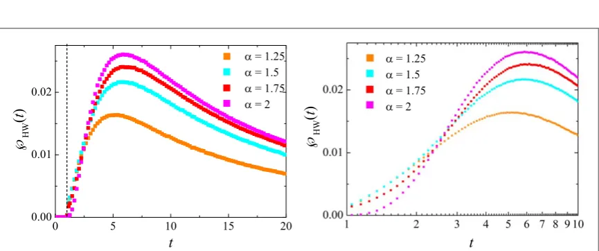
Naturally, the short-time properties of thefirst-hitting behaviour depicted infigure12for LWs differ from the corresponding shape for LFs, in analogy to our observations for thefirst-passage case. Namely, nofi rst-hitting event can occur before the LW front reaches the target. Then a jump in the value occurs att=x0/v0.

Similar to our discussion of thefirst-passage time PDF we attempted to insert an effective diffusion coefficient

KaLWin the known long-time expressions for LFs, equation(E.7). Given that this did not succeed for thefi rst-passage scenario, it is not surprising that an effective description in terms of LFs cannot approximate the LW behaviour.

6. Conclusions

LFs and LWs are broadly used models for efficient random search processes. In this paper we systematically analysed and compared thefirst-passage andfirst-hitting properties for two different models of Lévy motion, namely, LFs and LWs. We demonstrated that forα>1 the results of these two models are qualitatively identical at long times due to thefinite average length of a relocation. The situation drastically changes forα<1 when the scaling of the PDFs heavily depends on the exact model(see the summary in table2). This difference does not come as a surprise in view of the strong difference of the propagators of the two models, particularly, thefinite propagation front of LWs. Nevertheless, having quantitative data for the associatedfirst-passage andfirst-hitting time PDFs is valuable for any concrete analysis of search models based on LFs and LWs.

itself through a strong dependence of the value of the PDF at this instant on the time resolution of the simulations. In essence we showed that it is important to know the entirefirst-passage orfirst-hitting PDF in order to reach fully quantitative conclusions.

It will be interesting to extend the results reported herein to higher dimensions and/or multiple target scenarios. Higher-dimensional LFs and LWs can be defined in different ways[59,60], and it is nota prioriclear whether the difference in definitions modifies the behaviour for thefirst-passage andfirst-hitting time PDFs. In the case of multiple targets, for instance, disks distributed randomly in a plane, the associatedfirst-passage and

first-hitting time PDFs to locate these disks would move this problem closer to biological reality. One might think of, as an example, a bee searching forflowers, a situation amenable to experiments[110]. Measuring the

first-passage andfirst-hitting time PDFs may help to put the LF foraging hypothesis on more rigorous theoretical grounds, which is a long-standing open problem.

Another interesting direction to study is the combination of Lévy-type processes with resetting, as studied, for instance, for meanfirst passage and arrival times in[111]. Moreover, it will be interesting to explore in more detail the impact of a bias on thefirst-passage andfirst-hitting time PDFs similar to the analyses in[80,81]. Biologically this would relate to the problem of chemotaxis when cells migrate according to a chemical concentration gradient tofind inflammation sites[112]. Similarly, extensions of the present results in general external potentialfields[113]should be studied, including phenomena such as barrier crossing, stochastic resonant activation, and noise-enhanced stability phenomena[114]. Further applications to pursue include population dynamics and biophysical models[115], as well as the modelling of the dynamics in Josephson junctions[116], to mention but a few stray examples. We moreover note that it should be analysed how

distributed transport parameters(such asK_α)may modify the results forfirst-passage andfirst-hitting, similar to what happens for Brownian processes[117]. Finally, it will be interesting to study more complex, many-body scenarios such as hunting inflocks[118].

Acknowledgments

VVP acknowledges fruitful discussions with Olivier Bénichou. RM and AVC acknowledgefinancial support

from Deutsche Forschungsgemeinschaft(Grant numbers ME 1535/6-1 and ME 1535/7-1). RM also acknowledges an Alexander von Humboldt Honorary Research Scholarship from the Foundation for Polish Science. NW and GB were funded at Potsdam and Dresden, respectively, by ONR Global NICOP grant N62909-15-1-N143 to the CFSA, University of Warwick, and they wish to thank the PI, Sandra Chapman. RK thanks Sabine Klapp and Holger Stark, TU Berlin, for their hospitality as a guest scientist as well as ONR Global for

financial support. He also acknowledges funding from the London Mathematical Laboratory, where he is an

External Fellow. We acknowledge the support of Deutsche Forschungsgemeinschaft(German Research

Foundation)and Open Access Publication Fund of Potsdam University.

Appendix A. Short-time behaviour of the

fi

rst-passage of L

é

vy

fl

ights

Thefinite valuepjumpof the jump in the short-time behaviour of LFs(figure4)can be estimated by computing

the survival probability at short times by using the asymptotic expression for largex. For the purpose of this derivation we assume that the starting position is atx=0 while the boundary is atx=x0, which is physically

identical to our original setting. The survival probability at short times reads

t x0 f t x, d ,x A.1

S =

ò

( ) ( ) ( )

where the symmetric Lévy stable PDF in the limit∣ ∣x  ¥is[37,56]

f t x C K t

x C

, 1 a ₁ , 1a 1sin 2 1 . A.2

p pa a

~ = G +

a( ) ( )_{∣ ∣}a+a ( ) ( ) ( ) ( )

Thefirst-passage time density is the negative derivative of the survival probability,

t t

t

d

d . A.3

PF S

à ( )= - ( ) ( )

Conversely,

t f t x x C K t x

1 , d . A.4

x

1 0

0

S

ò

a

- = _a = a

a ¥

p dx f t x f, t x, d .x A.7

x

x x

2 1 1 1 2 2 2

0

0 1

ò

ò

= _a D _a D

-¥

-¥

( ) ( ) ( )

For simplicity we assume thatΔt1=Δt2. Then,

p x f t x f t x x

x f t x f t x x

x f t x f t x x

x f t x f t x x

x f t x f t x x

x f t x f t x x

p p x f t x f t x x

d , , d

d , , d

d , , d

d , , d

d , , d

d , , d

d , , d . A.8

x x

x x x

x

x x x

x x

x x x

x

x

x x x

2 1 1 1 1 2 2

1 1 1 1 2 2

1 1 1 1 2 2

1 1 1 1 2 2

1 1 1 1 2 2

1 1 1 1 2 2

1 1 2

1 1 1 1 2 2

0 1

0 0 1

0

0 1

0

0 0

0 0 1

0 0 0 1 0

ò

ò

ò

ò

ò

ò

ò

ò

ò

ò

ò

ò

ò

ò

= D D

- D D

= D D

+ D D

- D D

- D D

= - + D D

a a a a a a a a a a a a a a -¥ ¥ -¥ ¥ -¥ -¥ ¥ ¥ -¥ ¥ -¥ ¥ ¥ --¥ -( ) ( ) ( ) ( ) ( ) ( ) ( ) ( ) ( ) ( ) ( ) ( ) ( ) ( ) ( )

The latter integral can be computed analytically as follows,

x f t x f t x x

C K t

d , , d

1 . A.9

x

x x x

x x

x _{x x} x

x x

C K t x

x

x _x

x x

C K t x

x

x x

1 1 1 1 2 2

1 1 2 d d

1 d 1 1 d 1 d 1 1 0 0 1 0 0 1 11 0 1 0 2 21

1 12

02 1 11 1 2 21

1 12

02

1

11 1

ò

ò

ò

ò

ò

ò

ò

a a a

a

a a a

+ + + + +

(

)

In order to get an analytical result for the last integral we will split it into two parts from-¥to 0 and from 0 to 1. Thefirst part without the prefactor is

z z

z z z z B

1

1 d

1 d 2 , , A.10

x x x y y y y z 0 d 1 1 0

d 1 1 1 0 1 1 1 1 0 2 1 1

11 1

1

ò

ò

ò

ò

-= = -= + - = -¢ ¢ ¢ a

a a a

-¥ -¥ _{- +} + ¥ -+ ¥ - - -a a a a a a + +

(

)

(

)

(

)

y y zy y zu

F z

1

1

lim 1

lim 1 1 d 1

lim 1 , 1 , 2 ; , A.11

x x x y y y z y zy y

z z u

u

z z z z

0 1 d 1 1 0 1 d 1 1 1 0 1 _d 1 1 1 0 1

1 1 2 1 1 1 1

0 1

1 1 2 2 1

1 1 1 1 1 1 1 1 1 1

ò

ò

ò

ò

a a a

-= -= -= - - - -= + - - - + ¢ ¢ ¢

a a a a

a a

a

a a a

- - - + - - - -= =  G

-G -

-a a a a a a a + + + ⎧ ⎨ ⎩ ⎫ ⎬ ⎭

(

)

(

)

(

)

{

}

where2 1F(1+a, 1-a, 2-a;z)is the hypergeometric function obtained through the integral definition

which is valid in this case forα<1. This hypergeometric function can be transformed according to 15.3.6 from

[120]as follows

F z F z

z F z

1 , 1 , 2 ; 1 , 1 , 1 ; 1

1 1 2 , 1, 1 ; 1 . A.12

2 1 2 _{1 2} 2 1

2

1 1 2 1

a a a a a a

a a

+ - - = + - +

-+ - - -

-a a

a

a a a

a a

G - G G

-- G - G

G + G

-( ) ( ) ( ) ( ) ( ) ( ) ( ) ( ) ( ) ( ) ( ) ( )

Forz→1 the hypergeometric functions in the last expression will converge to 1. Assembling all of the pieces we obtain the following formula,

x x x d 1 1 1 1 1 1 2

1 4 1

1 2 . A.13

0 1

1

ò

G - =

-G -G -a a a + ⎛ ⎝ ⎜ ⎞ ⎠ ⎟ ( ) ( ) ( ) ( ) ( ) ( ) ( )

Finally, collecting all the contributions top2we get

p p p p

p p

p p

1

. A.14

2 1 1 2

1

2 4 1

1 2 1 2 1 1 2 4 1 2 1 2 1 1

2 4 1 2 cos 1 2 sin 2

3 2 = - + - -= + -= -p a a a a a p a a

a

a a

a

p pa

a a pa

G

-G

-G - G G G

-G

-G - G G +

G - G

a a a

(

)

(

)

The last expression clearly shows that with decreasingαatα=2/3 the probability to cross the boundary within an interval of time(Δt1, 2Δt1)gets lower thanp1due to the change in sign of the second term in(A.14). Thus,

t

PF

à ( )decreases forα<2/3 at shorttand atfirst grows forα>2/3.

Appendix B. Derivation of the average time of jump, the jump duration distribution and

its long-time expansion for L

é

vy walks, 1



<

α

„



2

In order to estimate the effective diffusion coefficient of LWs one has to know the distribution of durations of the jumps, the average jump duration as well as its long-time behaviour. The characteristic function of a symmetric Lévy stable process is

k exp ₀k . B.1

f_{( )}= ₍-sa_{∣ ∣ )}a _{( )}

The distribution of the jump lengths can be expressed in terms of FoxH-functions as[15,121]

f x k kx

xH x

d

cos e 1

2

1, 1

, , 1, .

k

0 12

11 0

1

2 2 2

0

ò

= =

a s

a

a a a a

¥

- a a ⎡

⎣ ⎢ ⎢ ⎤ ⎦ ⎥ ⎥

(

) (

)

The jump duration is coupled to the jump length distribution, x x

v0

t( )= . Then the relocation time

distribution reads

x x f x x f x

x f x x f x

x f x v f v

d d

d d

2 d 2 . B.2

x v x v x v x v 0 0

0 0 0

0 0 0 0

ò

ò

ò

ò

ò

y t d t t d t

d t d t

d t t

v

v v

2 2 , 1 1 1

1 1

4 2

1 1 , B.4

0 2 2 0 0 1 1 2 0 0 a p s a a p s s p a

= G +

-= G

-G - = G

-a a a a a a ⎜ ⎟ ⎛ ⎝ ⎜ ⎞_⎠⎟ ⎡ ⎣ ⎢ ⎢ ⎤ ⎦ ⎥ ⎥ ⎛ ⎝ ⎞⎠

( )

( )

using the properties of theH-function[121]. Our result exactly coincides with equation(54)in[57], where it was derived as an approximate formula. We show here that it is actually an exact expression(the factorv0missing in

the corresponding equation of[57]is just a misprint there). From the distribution we obtain the exact form in Laplace space and expand it at smallscorresponding to long times. The Laplace transform of equation(B.2) reads[121]

s H

H v s

H

v s

1, 1

, , 1,

2 2

1, , 1, 1

, , 1,

2 2 , , 0,

0, , 0, 1

. B.5

v

2

1211 ₂ 1

2 2 2

2212 0 0

1

2 2 2

2221 0 0

1

2 2 2

0

0

Ly t y L t

p s a p s a = = = =

p t s a a a

a

a a a a a

a a a a a a -a a a ⎛ ⎝ ⎜ ⎜ ⎡ ⎣ ⎢ ⎢ ⎤ ⎦ ⎥ ⎥ ⎞ ⎠ ⎟ ⎟ ⎡ ⎣ ⎢ ⎢ ⎤ ⎦ ⎥ ⎥ ⎡ ⎣ ⎢ ⎢ ⎤ ⎦ ⎥ ⎥

(

) (

)

(

) (

)

(

) (

)

The expansion of the latterH-function fors0has a ratio of nominally infinite values due to the presence of zeros among the coefficients. In order to solve this problem we introduce the infinitesimal parameterεand treat theH-function as a limit of anotherH-function with non-zero coefficientsε, namely,

H

v s H v s

2 , , 0,

0, , 0, 1

lim 2 , , ,

, , , 1

. B.6

2221 0 0

1

2 2 2

0 22 21 0

0

1

2 2 2

s

a

s e

e a e

= a a a a a a e a a a a a a  ⎡ ⎣ ⎢ ⎢ ⎤ ⎦ ⎥ ⎥ ⎡ ⎣ ⎢ ⎢ ⎤ ⎦ ⎥ ⎥

(

) (

)

(

) (

)

The expansion of the latterH-function reads([119,121]),

H z k k k z k k k k z k , , ,

, , , 1

2 ₁ 2 ₁ , B.7 k k k k k k 2221 1

2 2 2

0 1 1 2 1 2 1 2 0 1 2 1 2 1 2

å

å

e e e

p e e a

e a e e

p e e

= G - + G + +

G - +

-+ G - + G + +

G - +

-a a

a e a

e = ¥ + = ¥ + ⎡ ⎣ ⎢ ⎢ ⎤ ⎦ ⎥ ⎥

(

) (

)

(

) (

)

(

)

(

)

(

)

wherez=2a a as0s (v0a). Using the known behaviour of the Gamma function for small arguments,Γ(ε)∼1/ε,

we obtain the following expansion,

s 1 s As , B.8

y_{( )}~ - á ñ +t a+¼ _{( )}

where 1 has contributions from zeroth orders of both sums,á ñt is given by expression(B.4), andAreads

A

v v

2 1 2 2

2 cos 2 . B.9

1 0 0 0 0 s p a a a s pa

= - G - G +

G - =

a a a a a + _{( ) ( )} ( ) ∣ ( )∣ ( )

Appendix C. Derivation of the effective long-time diffusion coef

fi

cient of

LWs, 1



<

α

„



2

Let us start from equation(29)in[20],

P k s s kv s kv P k s kv s kv

, i i

2 i i , C.1

0

y y

= Y + + Y

-- + +

-( ) [ ˜ ( ) ˜ ( )] ( )

[ ( ) ( )] ( )

whereY˜ ( )s is the Laplace transform of the survival probability and can be expressed throughψ(s)as

s 1 y s s

Y˜ ( ) =[ - ( )] , and for long times(smalls)we havey( )s ~ - á ñ +1 t s Asa. Hence,

P k s P k A s kv s kv

s A s kv s kv

, 2 i i

2 i i . C.2

0 t 1 1

t

~ á ñ - + +

-á ñ - + +

-a a

a a

-

-( ) ( )[ (( ) ( ) )]

(( ) ( ) ) ( )

The expressions in the round brackets can be expanded,

s kv k v s

kv

i e 1

i . C.3

0

i

2 a

 a ~ pa a a 

⎜ ⎟ ⎛ ⎝ ⎞ ⎠ ( ) ∣ ∣ ( )

The last expansion assumes the conditions∣ ∣k v01. After neglecting higher powers insone gets

P k s P k

s A k v

,

cos

. C.4

0

0 ₂ t

=

- a a

_{( )}

( ) ( )

∣ ∣

( )

Alternatively,

P k s P k s K k

, , C.5

LW

0

=

+ _a a

( ) ( ) ∣ ∣ ( ) where K , C.6 Av v

LW cos 2 sin 1 cos sin 1 cos

1

0 ₂ 0 _{2 2}

0 1 _{2 2} 0

1 0 = = = = a _t

s a a

p t

s a a

s t

á ñ

G - G + á ñ

G - G +

G

-á ñ

a pa a pa pa

a pa pa

a a

-( )

( )

( )

( )

( )

(

)

whereá ñt is given by equation(B.4). The last result is exactly the intuitive definition of the diffusivity from a continuous time random walk perspective. The second line in equation(C.6)corrects the formula(55)in[57].

Appendix D. Estimation of the jump in the

fi

rst-passage time PDF of LWs

The jump in thefirst-passage time PDF of LWs corresponds to the probability stored in the ballistically moving front peak of the position PDF[20]. The density of particles in these peaks reads(equation(32)in[20])

G x t, 1 t x vt x vt

2 . D.1

front( )= Y( )( (d - )+d( + )) ( )

From the equations above we can compute the survival probability as a function of time. In Laplace space

s 1 y s s

Y˜ ( )=[ - ( )] . From expression(B.5),

s

s sH v s

2 2 , , 0,

0, , 0, 1

. D.2

2221 0 0

1

2 2 2

y

p

s

a

= ⎡ a a_a a a a

⎣ ⎢ ⎢ ⎤ ⎦ ⎥ ⎥

(

) (

)

Its inverse Laplace transform reads[121],

H t

H v t

, , 0, , 1,

0, , 0, 1

2 2

1, , 1, 1

, , 1, , 0, . D.3

s

s v

1 2

3221 2

1

2 2 2

2312 0 0

1

2 2 2

0 0 L a a p s a a = = y p

s _a a a

a

a a a a a

- a a

front

the series(D.5)converges quite fast.

Appendix E. Derivation of the long-time limit of the

fi

rst-hitting time PDF of

LFs, 1



<

α

„



2

We start from equation(9). The integral in the numerator can be computed analytically and reads

k

s K k

s K

d 1 2

sin . E.1

1 1 1

ò

a a a aa -¥ ¥ -∣ -∣ ( ) ( )

Hence equation(9)can be rewritten as

s K k s

s K k kx

sin

d cos . E.2

HF 1 0 1 1 0

ò

a p a p

à =

+

aa a

a a

¥

-( ) ( )

∣ ∣ ( ) ( )

From the relation(1.80)in[122]we know that

t E at s

s a, E.3

1

, - ¸

+ b

a b a

a b

a

- _{( )} - _{( )}

where÷stands as a notation for the Laplace transform pair andEα,β(t)is the two-parameter Mittag-Leffler

function. Hence, we get equation(10),

t sin K t d cosk kx E K k t . E.4

HF

1

1 1

0 0 1,1

ò

a p a p

à = a a a

-a a a

- ¥

( ) ( ) ( ) ( ) ( )

This equation clearly shows that forα=1 the PDF offirst-hitting the target is exactly zero,ÃHF=0(the prefactor is equal to zero in this case). Now we consider the long-time limitt ¥. Rewriting the previous equation as

t t kE K k t

t k kx E K k t

d

d 1 cos . E.5

K

K

HF sin 1 1

0 1,1 sin _{1 1}

0 0 1,1

1

1

ò

ò

à =

-- -

-a p a

p a a a a

a p a

p

a

a a a

- ¥ - ¥ aa aa ( ) ( ) ( ( )) ( ) ( ) ( ) ( )

Consider separately thefirst and the second contribution. Thefirst integral is zero,

kE K k t K t k E k

K t y E y y

y E y y

z E z

z

d d

d

lim d

lim

lim 0, E.6

z z z z z 0 1,1 1 0 1,1 1 1 0 1 1 1,1 0 1 1 1,1 1 1,1 1 1 1

ò

ò

ò

ò

a a a a a a a

a a a a a

a a a a a ¥ - ¥ - ¥ -¥ -¥ + ¥ ( ) ( ) ( ) ( ) ( ) ( ) ( ) ( )

where we used formula(1.99)in[122]. In the second integral the Mittag-Leffler function can be substituted by its large argument limit,E1,1 a(-K k ta a ) -1 [K k ta aG(1 a-1)], because at small values ofkthe expression

kx

1-cos 0

t k

x K t

x K t

d , E.7 K t kx k HF sin

1 1 ₀

1 cos sin

1 1

2 sin 1 0

1 1 1 1 2 sin 2 sin

1 0

1 1 1 1 2

1 1 1 2 0 2 2

ò

à =

= -= a p a a p a a a a

aa a

a

p a

a

a a a

G -¥ -G G -- - G -G - - -p a aa

a a p a pa p a pa

-( )

( )

( )

( )

( )

which exactly coincides with result(A.9)in[61]and is equivalent to the corresponding expression in[98].

Appendix F. Derivation of the short-time limit of the

fi

rst-hitting time PDF of LFs

Here we compute the power-law of thefirst-hitting time PDF of LFs in the limit of short times. It is again convenient to start from equation(10). We change the variable asy ₌k K t 1

a a

( ) . Hence,

t t y yx

K t E y

sin

d cos . F.1

HF 1

0

0 1 1,1

ò

a p a p

à =

-a a a

a - ¥ ⎛ ⎝ ⎜ ⎞ ⎠ ⎟ ( ) ( ) ( ) ( ) ( )

Introducing the notationl=x0 (K ta )1 aand using the definition of the Mittag-Leffler function,

t t y y

t y y I t

d cos

d cos , F.2

n y n n y n n n

HF sin 1

0 ₀ 1

sin 1

0 0 1 0

n n

ò

ò

å

å

å

a p a

p a

a p a

p a - ¥ = ¥ -G + -= ¥ ¥ -G + = ¥ a a ( ) ( ) ( ) ( ) ( ) ( ) ( ) ( ) ( ) ( ) ( )

whereIn(t)is thenth term of the expansion ofÃHF( )t in a power series. With the help of equation(2.25)for

improper integrals in[123],

k

e d 1 e F.3

k k k 0 i 1 1 i 1 2

ò

w

= G +

wt p ¥ -+ - + ( ) ( ) ( )

we compute the terms one by one. For convenience we use the shorthand notationC( )a = asin_p(p a). Then,

I t C t y y

I t C t

C t

C t

C t

d cos 0,

Re i

Re exp 1

sin

, F.4

K x

0 1 ₁1

0

1 1 ₁ 1₁ 1 1

1 1 1 1 1 i 2 1 1 1 1 1 2 1 sin 2

1 1 1 1 1 1 1 1 0 1

ò

G + ₊

- -G + G + - -G + G + G + G + a a a a a a + + + + + ⎡ ⎣

(

)

( )

I t C K

x t

2 1

2 1 sin , F.5

2

2 1 02 1

1 1

a a

a pa

= G +

G +

-a a a a + + + ( ) ( ) ( ) ( )( ( )) ( )

I t C K

x t

3 1

3 1 sin 3 2 . F.6

3

3 1 03 1

2 1

a a

a pa

= G +

G +

-a a a a + + + ( ) ( ) ( ) ( )( ( )) ( )

Appendix G. The target size selection in the simulations

Our theoretical framework for LFs includes the notion of a point-like target. However, in the simulations the target size should be non-zero if the target is to be successfully located. Thus the target should not be too small such that it can actually be hit successfully. At the same time it should not be too large, otherwise this would result in the scenario of thefirst-passage, and thus the scaling exponent would converge to the universal Sparre-Andersen result. One has to choose the target size correctly. From the theory the asymptotic behaviour at long times is known to beÃHF( )t t1 a-2[98]. InfigureG1we show how the exponent at long times depends on the

target size for the time resolutionδt=0.001. For very small targets the exponent is closer to−1(data 1 infigure G1)and the Sparre-Andersen limit can be obtained when large targets are considered(data set 4 infigureG1 corresponds to the case in which the starting point was distance 1 away from the boundary of the target with