Fusion of Landsat 8 OLI and Sentinel-2 MSI data
Qunming Wang a, George Alan Blackburn a, Alex O. Onojeghuo a, Jadu Dash b, Lingquan Zhou b, Yihang Zhang c,d, Peter M.
Atkinson b,e,f
a Lancaster Environment Centre, Lancaster University, Lancaster LA1 4YQ, UK
b Geography and Environment, University of Southampton, Highfield, Southampton SO17 1BJ, UK c Institute of Geodesy and Geophysics, Chinese Academy of Sciences, Wuhan 430077, China
d University of Chinese Academy of Sciences, Beijing 100049, China
e Faculty of Science and Technology, Engineering Building, Lancaster University, Lancaster LA1 4YR, UK f School of Geography, Archaeology and Palaeoecology, Queen's University Belfast, BT7 1 NN, Northern Ireland, UK
E-mail: wqm11111@126.com
Abstract: Sentinel-2 is a wide-swath and fine spatial resolution satellite imaging mission designed for data continuity and enhancement of the Landsat and other missions. In this paper, a new approach is presented for fusion of Landsat 8 and Sentinel-2 data to coordinate their spatial resolutions for continuous global monitoring. The advanced area-to-point regression kriging (ATPRK) approach was employed for the fusion problem, where the 30 m spatial resolution Landsat 8 bands are downscaled to 10 m using 10 m Sentinel-2 bands as covariates. To account for the land-cover/land-use (LCLU) changes that may have occurred between the Landsat 8 and Sentinel-2 images, the Landsat 8 PAN band was also incorporated in the fusion process. The experimental results showed that the proposed approach is effective for fusing Landsat 8 with Sentinel-2 data, and the use of the PAN band can decrease the errors introduced by LCLU changes. By fusion of Landsat 8 and Sentinel-2 data, more frequent observations can be produced for continuous monitoring, and the observed 30 m Landsat 8 data can be downscaled to a finer spatial resolution of 10 m. The products have great potential for timely monitoring of rapid changes on the Earth’s surface.
Keywords: Landsat 8, Sentinel-2, image fusion, downscaling, area-to-point regression kriging (ATPRK), global monitoring.
1. Introduction
Landsat data have been used widely for global monitoring, due to their free availability and regular revisit capabilities. The Landsat 5 satellite equipped with Thematic Mapper (TM) sensor was launched in 1984, but the TM sensor stopped transmitting in November 2011. As the successor of Landsat 5, the Landsat 7 satellite was launched in April 1999. In May 2003, however, the scan-line corrector (SLC) of the Landsat 7 Enhanced Thematic Mapper Plus (ETM+) sensor failed permanently, resulting in SLC-off images with around 22% dead pixels from May 2003 to present [1]. To cope with the SLC-off issue of the Landsat 7 ETM+ sensor, the new generation Landsat 8 satellite equipped with Operational Land Imager (OLI) and Thermal Infrared Sensor (TIRS) sensors was launched in February 2013 and the sensors are now in operation routinely acquiring global remote sensing data [2]. The limitation of Landsat is that the satellites can only revisit the same area every 16 days. In most cases, the acquired Landsat data for specific areas can be contaminated by cloud and shadow, meaning that obtaining one clean Landsat image per month is considered a good outcome [3]. The temporally sparse time-series Landsat data are, therefore, unsuitable for global monitoring of rapid changes on the Earth’s surface, such as urbanization (especially in highly developed cities, such as Shenzhen in China) [4]-[5], deforestation and forest degradation (such as in the Amazon rainforest) [6], and rapid phenology changes (e.g., due to crop harvesting) [7].
spatio-temporal fusion methods require at least one pair of MODIS-Landsat images acquired on the same day to guide the downscaling process of MODIS on other days [8]-[10]. This can be demanding for a given period. Moreover, from the observed spatial resolution of 500 m to the target resolution of 30 m, the downscaling process involves a large zoom factor of 16, indicating large uncertainties given the ill-posed nature of the problem. In addition, the difference between the geographic coordinate system of MODIS (in the Sinusoidal projection) and Landsat (in the UTM/WGS84 projection) may potentially lead to additional uncertainties in downscaling.
Very recently in June 2015, the Sentinel-2 satellite was launched for data continuity and enhancement of the Landsat and SPOT missions. Sentinel-2 is a wide-swath and fine spatial resolution satellite imaging mission of the European Space Agency (ESA) developed in the framework of the European Union Copernicus programme [14]-[16]. Sentinel-2 data cover 13 spectral bands, with four bands at 10 m, six bands at 20 m and three bands at 60 m spatial resolution. The sensor revisits the same area every ten days with a constant viewing angle. The free access, fine spatial resolution, global coverage and fine temporal resolution make the Sentinel-2 data of great utility for a wide range of applications based on remote sensing.
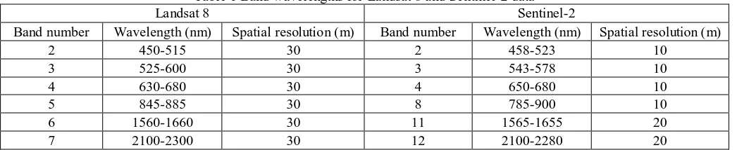
[image:2.612.47.570.363.470.2]The Sentinel-2 bands have corresponding wavelengths to the Landsat bands; see the example for Landsat 8 and Sentinel-2 data in Table 1 [17]. Moreover, the Sentinel-2 products published online have the same geographic coordinate system as Landsat products. The free access of both Sentinel-2 and Landsat data, the same wavelengths, and the same geographic coordinate system provide an excellent opportunity to combine these two types of data for more continuous monitoring at the global scale. As seen from Table 1, however, the spatial resolutions of the two types of data are different and Sentinel-2 has finer spatial resolutions (10 and 20 m) than Landsat (30 m).
Table 1 Band wavelengths for Landsat 8 and Sentinel-2 data
Landsat 8 Sentinel-2
Band number Wavelength (nm) Spatial resolution (m) Band number Wavelength (nm) Spatial resolution (m)
2 450-515 30 2 458-523 10
3 525-600 30 3 543-578 10
4 630-680 30 4 650-680 10
5 845-885 30 8 785-900 10
6 1560-1660 30 11 1565-1655 20
7 2100-2300 30 12 2100-2280 20
In this paper, for the first time, we fuse Landsat 8 and Sentinel-2 data by addressing the incompatibility problem of spatial resolution to achieve potentially continuous monitoring. There are two potential schemes for the fusion task. The first is to upscale the 10 or 20 m Sentinel-2 data to 30 m to match the spatial resolution of Landsat 8. This scheme is straightforward, but wastes the valuable 10 m information obtained by Sentinel-2. The second scheme is to downscale the 30 m Landsat 8 data to 10 m to match the spatial resolution of Sentinel-2. This scheme aims to take full advantage of the available information in both Landsat 8 and Sentinel-2. For global monitoring, analysts always prefer to obtain as much detailed spatial information as possible. In this paper, the second scheme is considered. Specifically, we downscale the 30 m bands 2-7 of Landsat 8 to 10 m, with the aid of 10 or 20 m resolution data in the corresponding Sentinel-2 bands 2, 3, 4, 8, 11 and 12. We suggest that the Sentinel-2 bands provide valuable information at the 10 m target spatial resolution, which can greatly decrease the uncertainty in downscaling Landsat 8 data. This downscaling issue is also termed image fusion in remote sensing. The significance of fusing Landsat 8 with Sentinel-2 data is twofold.
1) It can produce more frequent time-series images for continuous global monitoring. More precisely, in theory, every month Sentinel-2 can provide an additional three observations as supplementary information to the two Landsat observations, thus, increasing the number of observations every month to five.
a finer spatial resolution than the original Landsat data. Many features (e.g., urban fabric, small residential buildings, roads and other linear features) that cannot be observed clearly in the original 30 m Landsat data can be shown more explicitly in the 10 m downscaled products.
Over the past decades, various approaches have been developed for image fusion, such as the intensity-hue-saturation [18], Brovey [19], principal component analysis [20], a trous wavelet transform (ATWT) [21], high-pass filter (HPF) [22], smoothing filter-based intensity modulation (SFIM) [23], and sparse representation [24] methods. There are several reviews of the available image fusion approaches
[25]-[28]. Recently, area-to-point regression kriging (ATPRK) in geostatistics was proposed for image fusion
[29], [30]. ATPRK treats the coarse band as the primary variable and the fine spatial resolution band (hereafter, fine band) as a covariate. It is an advanced image fusion approach which has the appealing advantage of precisely preserving the spectral properties of the observed coarse images (i.e., perfectly coherent). The advantages of ATPRK over other geostatistical approaches (such as kriging with external drift [31] and downscaling cokriging [32]-[34]) have been presented both theoretically and experimentally in our previous research [29], [30]. ATPRK is a user-friendly approach and accounts explicitly for size of support (pixel), spatial correlation, and the point spread function (PSF) of the sensor. Motivated by the advantages and encouraging performance of ATPRK in our previous research, in this paper, ATPRK is employed for fusion of Landsat 8 and Sentinel-2 data.
When fusing Landsat with Sentinel-2 data, land-cover/land-use (LCLU) changes may have taken place during the period of time between the acquisition of both datasets and this can be a critical problem bringing great challenges. This is prominent when abrupt changes occur from Sentinel-2 to (relatively) coarse Landsat images. For example, hypothetically, in a Sentinel-2 image a region may be entirely covered by bare soil, but in a Landsat 8 image some parts of the region may be changed to be mixed with both bare soil and small residential buildings (smaller than 30 m). In this case, the 10 or 20 m Sentinel-2 image of this region cannot provide useful spatial information for downscaling the Landsat data (e.g., downscaling the small residential buildings that cannot be observed by Sentinel-2 at all). Therefore, using only the Sentinel-2 image may sometimes be insufficient for accurately reproducing the LCLU changes that have occurred between the acquisition time of the Landsat and Sentinel-2 data.
It is worth noting that the Landsat 8 OLI sensor also provides a 15 m panchromatic (PAN) band (band 8) covering the same scene with the 30 m multispectral bands. Although coarser than the 10 m target spatial resolution, the PAN band is acquired at the exactly same time with the 30 m multispectral bands and can reveal the changes at a finer spatial resolution than 30 m which may not be observed by the 10 m Sentinel-2 image (e.g., the abrupt changes). In this paper, we fuse Landsat 8 with Sentinel-2 data by taking full advantage of all the available information provided by the two types of sensors. Specifically, based on the advanced ATPRK approach, we propose a new fusion approach to incorporate 10 or 20 m Sentinel-2 and 15m PAN images to downscale 30 m Landsat 8 images to 10 m.
The remainder of this paper is organized as follows. Section 2 first briefly introduces the theoretical basis of ATPRK, and then the principles of the proposed ATPRK-based fusion approach. The experimental results are provided in Section 3 to demonstrate the applicability of the proposed fusion approach. Section 4 provides some further discussions, followed by a conclusion in Section 5.
2. Methods
2.1 ATPRK
Suppose Z xVl( )i is the random vector of pixel V centered at xi (i=1,…,M, where M is the number of pixels)
in coarse band l (l=1,…,L, where L is the number of coarse bands), and k( )
v j
Z x is the random vector of pixel v
centered at xj (j=1,…, 2
MF , where F is the spatial resolution (zoom) ratio between the coarse and fine bands)
in fine band k (k=1,…,K, where K is the number of fine bands). Using the primary variable Z xVl( )i at coarse spatial resolution and covariate Z xvk( j) at fine spatial resolution as inputs, ATPRK aims to predict the target
variable Z xvl( ) for all fine pixels in all coarse bands.
Denoting the predictions of the regression and the ATPK parts as ˆ ( )l1 v
Z x and ˆ ( )l2 v
Z x , the ATPRK prediction is given by
1 2
ˆl( ) ˆl ( ) ˆl ( )
v v v
Z x Z x Z x . (1) At a specific location x0, the regression prediction is a linear combination of the K fine pixels in K fine
bands
0
1 0 0 0
0
ˆ ( ) ( ), ( ) 1
K
l l k
v k v v
k
Z a Z Z
x x x . (2)
Assuming the relation in (2) is invariant with spatial scale, the coefficients {a kkl | 0,..., }K in (2) are
calculated according to the relationship between the observed coarse band l and the upscaled bands ZVk
(k=1,…,K) from the original K fine bands.
0
0
( ) ( ) ( ), ( ) 1
K
l l k l
V k V V V
k
Z a Z R Z
x x x x x (3)
where the coefficients are estimated by ordinary least squares [37]. R xVl( ) is a residual term that needs to be downscaled to the fine spatial resolution in the following.
ATPK is performed in the second-stage to downscale the coarse residuals R xVl( ) in (3) to the target fine spatial resolution. The fine residual at location x0 is predicted as
2 0
1 1
ˆ ( ) ( ), s.t. 1
N N
l l
v i V i i
i i
Z R
x x (4)
in which i is the weight for the ith coarse residual centered at xi and N is the number of neighboring coarse
pixels. The weights {i|i1,..., }N are calculated according to the kriging matrix
1 1 1
1 ( , ) ... ( , ) . . . . . . . . . . . ( , ) ... l l
VV VV N
l l
VV N VV
x x x x
x x 0 1 1 0 ( , ) . . . . . . ( , ) ( , )
1 ... 1
l vV
l N
N N vV N
x x
x x x x
(5)
where VVl ( ,x xi j) is the coarse-to-coarse semivariogram between coarse pixels centered at xi and xj in band
l, vVl (x x0, j) is the fine-to-coarse semivariogram between fine and coarse pixels centered at x0 and xj in
band l, and is the Lagrange multiplier. Suppose s is the Euclidean distance between the centroids of any two pixels and h sVl( ) is the PSF of the sensor. VVl ( )s and vVl ( )s are calculated by convoluting the fine-to-fine semivariogram vvl ( )s with the PSF ( )
l V
h s as follows
( ) ( ) * ( )
l l l
vV vv hV
s s s (6) ( ) ( ) * ( ) * ( )
l l l l
VV vv hV hV
calculated from the coarse residual image R xVl( ). Details on the deconvolution approach can be found in [29].
Based on the hypothesis that the coarse pixel value is the average of the fine pixel values within it, the sensor PSF can be defined as follows [32]-[34]
1
, if ( ) ( )
0, otherwise
V V
V
h S
x x
x (8)
in which SV is the size of pixel V and ( )V x is the spatial support of pixel V centered at x.
2.2 The proposed ATPRK-based approach for fusion of Landsat 8 and Sentinel-2
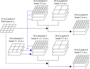
The proposed fusion approach makes full use of the information in 10 or 20 m Sentinel-2 bands, 30 m Landsat 8 multispectral bands and the 15 m Landsat 8 PAN band to produce 10 m Landsat 8 multispectral bands. This section introduces the principle of the ATPRK-based fusion approach.
As seen from Table 1, 20 m Sentinel-2 bands 11 and 12 have the same wavelength as 30 m Landsat 8 bands 6 and 7 and the former will be fused with the latter in downscaling. Obviously, the two 20 m Sentinel-2 bands need to be downscaled to 10 m in advance to provide the 10 m reference for Landsat 8 bands 6 and 7. For the downscaling process, the 10 m information in Sentinel-2 bands 2, 3, 4, and 8 can be used. This process can be achieved using the ATPRK approach, where the 10 m Sentinel-2 bands 2, 3, 4, and 8 are treated as fine bands (covariates). All four 10 m bands can be used straightforwardly in ATPRK by multiple regression in (2) and (3). However, the consideration of all fine bands in the regression model in ATPRK may over-generalize. In this paper, for each of the 20 m bands 11 and 12, a 10 m band with the greatest correlation (quantified by the correlation coefficient (CC)) with it was selected from the 10 m bands 2, 3, 4, and 8 and used as the covariate in ATPRK.
The wavelength of the Landsat 8 PAN band is 500-680 nm, which covers those of Landsat 8 bands 2-4 but not bands 5-7. Thus, compared with 10 m Sentinel-2 images, the Landsat 8 PAN image may not always be able to provide more useful spatial information for downscaling bands 5-7. On the other hand, if the LCLU changes between the Sentinel-2 and Landsat 8 images are large or the acquisition time of the two types of data is very different, using only Sentinel-2 bands 8, 11 and 12 that have the same wavelength with Landsat 8 bands 5-7 may also not be able to provide sufficient textural information at 10 m spatial resolution for the changed areas. Based on this hypothesis, in the proposed fusion approach, Landsat 8 bands 2-4 are downscaled using both Sentinel-2 (corresponding bands 2-4) and Landsat 8 PAN images as auxiliary data. For Landsat 8 bands 5-7, Sentinel-2 images are still used for fusion as they provide spatial information at the desired 10 m spatial resolution, which is particularly valuable for unchanged areas. However, whether the Landsat 8 PAN image should be considered for Landsat 8 bands 5-7 depends on its correlation with them. Fig. 1 illustrates schematically the fusion approach.
For the lth (l=5, 6 and7) band of Landsat 8, we denote the CC between the band and the Landsat 8 PAN band as CC L L( ,l PAN), and the CC between the band and the corresponding kth Sentinel-2 band (k=8, 11 and
12) as CC L S( ,l k). If CC L L( ,l PAN)>CC L S( ,l k), the PAN image is used in fusion; otherwise, the PAN image is not considered as helpful auxiliary data and only the Sentinel-2 images are used. Note that before calculating the CCs, the Landsat 8 PAN band and Sentinel-2 bands 8, 11 and 12 need to be upscaled to 30 m to match the spatial resolution of the Landsat 8 bands 5-7.
The proposed fusion approach is, thus, implemented as follows.
1) Based on ATPRK, the 20 m Sentinel-2 bands 11 and 12 are downscaled to 10 m using the 10 m bands 2, 3, 4, and 8 as covariates. For each 20 m band, a 10 m band with the largest CC is selected from bands 2, 3, 4, and 8.
2) Based on ATPRK, the 30 m Landsat 8 bands 2-4 are downscaled to 15 m using the 15 m Landsat 8 PAN band as the covariate.
4) Treating the 5 m Sentinel-2 bands as covariates, the 15 m pan-sharpening results of step 2) are further downscaled to 5 m using ATPRK. In this process, each 15 m band of Landsat 8 is downscaled using the 5 m band with the same wavelength (see Table 1).
5) The 5 m results of step 4) are upscaled to 10 m to produce the final results for Landsat 8 bands 2-4. 6) For Landsat 8 bands 5-7, the CCs between them and the Landsat 8 PAN band (i.e., CC L L( ,l PAN), l=5, 6
and7) and Sentinel-2 bands 8, 11 and 12 (i.e., CC L S( ,l k), k=8, 11 and 12) are calculated.
7) For the lth of Landsat 8 bands 5-7, if CC L L( ,l PAN)>CC L S( ,l k), the PAN image is used, and the downscaling process for this Landsat 8 band is similar to that for Landsat 8 bands 2-4 (see steps 2-5), where Sentinel-2 band 8, 11 or 12 is involved instead. Otherwise, only the corresponding 10 m Sentinel-2 band is considered as the covariate and fused with the 30 m band to produce the final 10 m downscaling result for this Landsat 8 band.
10 m Sentinel-2 bands 2-4 at t1
30 m Landsat 8 bands 2-4 at t2
10 m Sentinel-2 bands 8, 11, 12 at t1
30 m Landsat 8 bands 5-7 at t2
20 m Sentinel-2 bands 11, 12 at t1
15 m Landsat 8 PAN band at t2
10 m Landsat 8 bands 2-4 at t2
[image:6.612.125.490.234.514.2]10 m Landsat 8 bands 5-7 at t2
Fig. 1 The proposed image fusion approach for downscaling Landsat 8 multispectral bands 2-7 at t2, which
uses both a Sentinel-2 image at t1 and a Landsat 8 PAN image at t2 as auxiliary data. The blue lines indicate
that the Sentinel-2 bands 11 and 12 are downscaled to 10 m using the 10 m Sentinel-2 bands 2, 3, 4 and 8. The dashed line indicates that whether the Landsat 8 PAN image should be incorporated in downscaling Landsat 8 bands 5-7 depends on its correlation with them.
As the spatial resolution ratio between the 15 m PAN and 10 m Sentinel-2 bands is not an integer, step 3) of downscaling and step 5) of backward upscaling are introduced, which means that it is essentially 10 m Sentinel-2 information incorporated in the fusion process. The uncertainty in downscaling in step 3), which involves direct interpolation without auxiliary data, can be eliminated by the upscaling process in step 5).
information at 30 m spatial resolution is precisely preserved. Note that when no LCLU changes occur between Sentinel-2 and Landsat 8 observations, using only Sentinel-2 image as the covariate would lead to almost the same performance as using both Sentinel-2 and Landsat 8 PAN images as covariates.
3. Experiments
3.1 Data and experimental setup
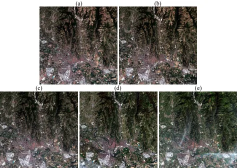
In the experiments, the Landsat 8 and Sentinel-2 datasets used cover a scene in Verona, Italy. The study area has a spatial extent of 18 km by 18 km, and correspondingly, the 30 m Landsat bands contain 600 by 600 pixels, the 15 m Landsat PAN band contains 1200 by 1200 pixels, and the 10 m Sentinel-2 bands contain 1800 by 1800 pixels. The study area is covered mainly by a mix of vegetation and urban fabric. The Sentinel-2 data were acquired on 18 August 2015. They are Level-1C products and provide geo-coded top of atmosphere reflectance with a sub-pixel multispectral registration in the UTM/WGS84 projection [14]. As for Landsat 8 datasets (multispectral bands 2-7 and PAN band 8), we used four observations acquired on 6 September 2015, 5 August 2015, 10 April 2015, and 1 November 2014, respectively. All Landsat 8 datasets are also in the UTM/WGS84 projection. The original digital number was converted to top of atmosphere reflectance using the radiometric rescaling coefficients and Sun angle provided in the product metadata file [38]. The Sentinel-2 and Landsat 8 images are shown in Fig. 2. As observed from the bottom right corner of the five images, obvious LCLU changes exist among all images.
(a) (b)
[image:7.612.69.547.355.691.2](c) (d) (e)
2015). (c) 30 m Landsat 8 image (5 August 2015). (d) 30 m Landsat 8 image (10 April 2015). (e) 30 m Landsat 8 image (1 November, 2014).
The 30 m Landsat 8 bands could be fused with the 10 m Sentinel-2 bands to produce the 10 m Landsat 8 images. However, no reference at 10 m could then be used to examine the performance of downscaling objectively. Thus, for reliable assessment, synthetic datasets were used in the experiments. More precisely, all available data were upscaled by a factor of three. Accordingly, the 30 m Landsat 8 bands, 15 m Landsat 8 PAN band and 10 m Sentinel-2 bands were upscaled to 90 m (200 by 200 pixels), 45 m (400 by 400 pixels) and 30 m (600 by 600 pixels). The objective of Landsat 8 and Sentinel-2 fusion was to reproduce the 30 m Landsat bands with the aid of the 45 m PAN and 30 m Sentinel-2 bands. With this scheme, the 30 m Landsat bands are known perfectly and can be used for objective assessment. This is a scheme used commonly in experimental studies to evaluate downscaling approaches [39].
The HPF [22], SFIM [23] and ATWT [21] methods were used as three benchmark methods for comparison. They fused directly the 90 m Landsat bands with 30 m Sentinel-2 bands to produce 30 m Landsat results. Moreover, three different versions of ATPRK were also implemented. The first one uses only 30 m Sentinel-2 data, while the second one uses only the 45 m PAN band (i.e., the standard pan-sharpening problem). The third one is the proposed fusion approach that uses both the Sentinel-2 and Landsat PAN images. For clarity, we denote the three versions as ATPRK1, ATPRK2, and ATPRK3. For ATPRK2, the 45 m image band with 400 by 400 pixels was first interpolated to 600 by 600 pixels to match the spatial size of the 30 m spatial resolution images. The interpolated PAN image was then fused with the 90 m Landsat 8 multispectral bands to produce 30 m predictions.
Six indices were used for quantitative assessment, including the root mean square error (RMSE), CC, universal image quality index (UIQI) [40], relative global-dimensional synthesis error (ERGAS) [41], spectral angle mapper (SAM) and coherence. For RMSE, CC and UIQI, they were first calculated for each band, and then the values for all bands were averaged. For SAM, values for spectra of all pixels were first calculated and then averaged. Coherence (quantified by the CC) is an index measuring the relation between the observed coarse image and the coarse image obtained by upscaling the sharpened image. For each multispectral band, a coherence value was calculated and the values for all bands were averaged.
3.2 Downscaling Landsat 8 images in the past
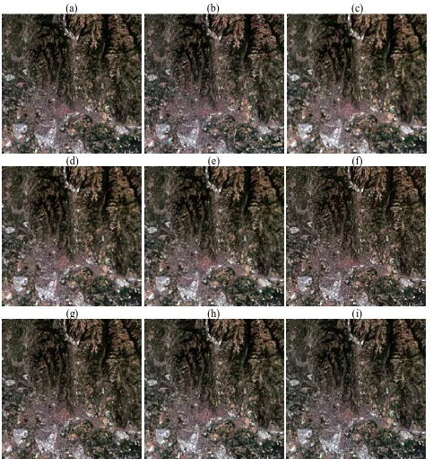
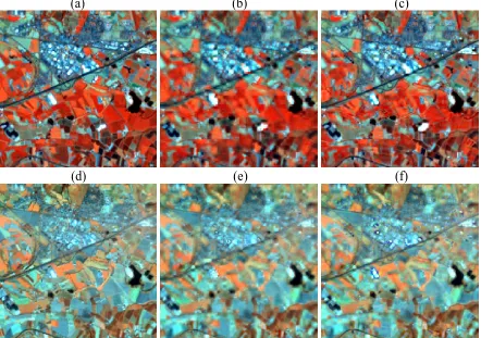
In this section, the 90 m Landsat data of 5 August 2015 were downscaled to 30 m. The acquisition time of the Landsat data is before that of Sentinel-2 (18 August 2015), and thus, can illustrate the performance of the proposed approach for downscaling Landsat images in the past (i.e., acquired earlier than Sentinel-2). The results are shown in Fig. 3 where bands 432 were selected as the RGB composite. For convenience of visual inspection, Fig. 4 shows the results for a 4.5 km by 4.5 km sub-area. From the date of Landsat 8 acquisition to Sentinel-2, the study area was subject to several LCLU changes; see the faint yellow objects in the Sentinel-2 image in Fig. 4(b). As shown in the results, the downscaling results are visually more satisfactory than the original 90 m coarse image in Fig. 4(c) and many details can be reproduced, suggesting the benefits of the fusion methods.
saturation artifacts produced by the LCLU changes and reproduce more accurately the LCLU boundaries (see again the faint yellow objects in the first few columns).
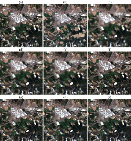
(a) (b) (c)
(d) (e) (f)
[image:9.612.67.550.104.615.2](g) (h) (i)
(a) (b) (c)
(d) (e) (f)
[image:10.612.87.527.106.579.2](g) (h) (i)
Fig. 4 30 m Downscaling results for a sub-area in Fig. 3 (bands 432 as RGB). (a) 30 m Landsat 8 reference (5 August 2015). (b) 30 m Sentinel-2 image (18 August 2015). (c) 90 m Landsat 8 image used as input (5 August 2015). (d) HPF result. (e) SFIM result. (f) ATWT result. (g) ATPRK result produced by fusing the 90 m Landsat image with the 30 m Sentinel-2 image (ATPRK1). (h) ATPRK result produced by fusing the 90 m Landsat image with the 45 m PAN image (ATPRK2). (i) ATPRK result produced by fusing the 90 m Landsat image with the 30 m Sentinel-2 and 45 m PAN images (ATPRK3).
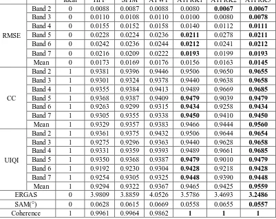
ATPRK3 products are more accurate than ATPRK2. This is because ATPRK2 uses only 45 m Landsat 8 PAN information in the fusion process, but ATPRK1 and ATPRK3 use the Sentinel-2 data which can provide information at the desired 30 m spatial resolution. Furthermore, ATPRK3 has a larger CC and UIQI and smaller RMSE, ERGAS and SAM than ATPRK1. More precisely, ATPRK3 reduces the overall RMSE, ERGAS and SAM by 0.0011, 0.3300, and 0.0001, respectively, and increases both the overall CC and overall UIQI by 0.0094. This demonstrates that incorporation of the Landsat 8 PAN band can enhance the performance of ATPRK in fusing Landsat 8 with Sentinel-2 data. It is noteworthy that ATPRK1 and ATPRK3 have the same performances for Landsat 8 bands 5-7. The reason for this is that the three bands have a larger correlation with Sentinel-2 bands 8, 11 and 12 than for the Landsat 8 PAN band, and according to the principle of the proposed ATPRK3 approach, the PAN band was not considered when downscaling these three bands.
Table 2 Quantitative assessment of the downscaling methods for the entire Landsat 8 image of 5 August 2015 (ATPRK1 uses only the 30 m Sentinel-2 data, ATPRK2 uses only the 45 m PAN band, and ATPRK3 uses both
the 30 m Sentinel-2 and 45 m PAN data; the bold values indicate the most accurate result in each term) Ideal HPF SFIM ATWT ATPRK1 ATPRK2 ATPRK3
RMSE
Band 2 0 0.0088 0.0087 0.0088 0.0080 0.0067 0.0067
Band 3 0 0.0110 0.0108 0.0110 0.0100 0.0080 0.0078
Band 4 0 0.0155 0.0152 0.0158 0.0140 0.0112 0.0111
Band 5 0 0.0228 0.0224 0.0236 0.0211 0.0278 0.0211
Band 6 0 0.0242 0.0236 0.0244 0.0212 0.0241 0.0212
Band 7 0 0.0216 0.0209 0.0222 0.0193 0.0199 0.0193
Mean 0 0.0173 0.0169 0.0176 0.0156 0.0163 0.0145
CC
Band 2 1 0.9381 0.9396 0.9446 0.9506 0.9650 0.9655
Band 3 1 0.9301 0.9324 0.9378 0.9440 0.9638 0.9658
Band 4 1 0.9355 0.9384 0.9413 0.9489 0.9669 0.9685
Band 5 1 0.9368 0.9387 0.9409 0.9479 0.9039 0.9479
Band 6 1 0.9263 0.9299 0.9315 0.9434 0.9258 0.9434
Band 7 1 0.9305 0.9355 0.9338 0.9450 0.9410 0.9450
Mean 1 0.9329 0.9357 0.9383 0.9466 0.9444 0.9560
UIQI
Band 2 1 0.9361 0.9375 0.9432 0.9506 0.9644 0.9654
Band 3 1 0.9275 0.9296 0.9363 0.9440 0.9628 0.9658
Band 4 1 0.9331 0.9359 0.9393 0.9489 0.9661 0.9685
Band 5 1 0.9350 0.9368 0.9387 0.9479 0.9010 0.9479
Band 6 1 0.9192 0.9230 0.9304 0.9428 0.9218 0.9428
Band 7 1 0.9254 0.9305 0.9325 0.9448 0.9390 0.9448
Mean 1 0.9294 0.9322 0.9367 0.9465 0.9425 0.9559
ERGAS 0 3.9809 3.8859 4.0526 3.5786 3.4693 3.2486
SAM(°) 0 0.0628 0.0615 0.0669 0.0558 0.0655 0.0557
Coherence 1 0.9961 0.9964 0.9862 1 1 1
3.3 Downscaling Landsat 8 images in the future
boundaries between the LCLU classes are much clearer than those in the other five results, and it is the closest to the reference in Fig. 5(a).
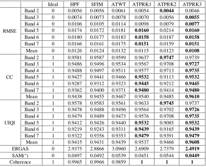
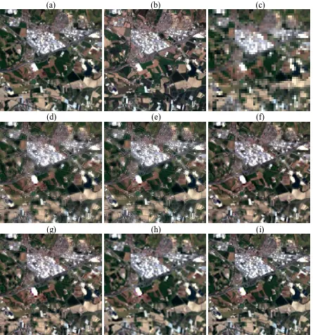
Table 3 displays the accuracies of all tested methods for the entire 18 km by 18 km study area. Similarly to visual inspection, the three ATPRK-based methods are more accurate than HPF, SFIM and ATWT. As for the inter-comparison between the three ATPRK-based methods, ATPRK2 is the least accurate. In this experiment, the Landsat 8 bands 5-7 also have a larger correlation with Sentinel-2 bands 8, 11 and 12 than for the Landsat 8 PAN band and, thus, the PAN band was not used for these three bands. As a result, ATPRK1 and ATPRK3 have the same performances for Landsat 8 bands 5-7. Using both PAN and Sentinel-2 data, however, ATPRK3 increased the overall CC and UIQI by 0.0070 and 0.0071, respectively. The accuracies of both ATPRK1 and ATPRK3 are greater than that in Table 2, and the accuracy gains of ATPRK3 over ATPRK1 is smaller than that in Table 2. This is because fewer LCLU changes occurred between the Sentinel-2 image and the Landsat image used in this experiment. This experiment reveals that the proposed approach also works well for downscaling Landsat images in the future.
(a) (b) (c)
(d) (e) (f)
Fig. 5 30 m Downscaling results for a sub-area of the Landsat 8 image on 6 September 2015 (bands 432 as RGB). (a) 30 m Landsat 8 reference (6 September 2015). (b) 30 m Sentinel-2 image (18 August 2015). (c) 90 m Landsat 8 image used as input (6 September 2015). (d) HPF result. (e) SFIM result. (f) ATWT result. (g) ATPRK result produced by fusing the 90 m Landsat image with the 30 m Sentinel-2 image (ATPRK1). (h) ATPRK result produced by fusing the 90 m Landsat image with the 45 m PAN image (ATPRK2). (i) ATPRK result produced by fusing the 90 m Landsat image with the 30 m Sentinel-2 and 45 m PAN images (ATPRK3). Table 3 Quantitative assessment of the downscaling methods for the entire Landsat 8 image of 6 September
2015 (ATPRK1 uses only the 30 m Sentinel-2 data, ATPRK2 uses only the 45 m PAN band, and ATPRK3 uses both the 30 m Sentinel-2 and 45 m PAN data; the bold values indicate the most accurate result in each
term)
Ideal HPF SFIM ATWT ATPRK1 ATPRK2 ATPRK3
RMSE
Band 2 0 0.0056 0.0056 0.0061 0.0054 0.0044 0.0046 Band 3 0 0.0074 0.0073 0.0078 0.0070 0.0056 0.0055
Band 4 0 0.0106 0.0105 0.0114 0.0098 0.0079 0.0077
Band 5 0 0.0174 0.0172 0.0181 0.0160 0.0214 0.0160
Band 6 0 0.0180 0.0177 0.0183 0.0158 0.0187 0.0158
Band 7 0 0.0166 0.0161 0.0175 0.0151 0.0159 0.0151
Mean 0 0.0126 0.0124 0.0132 0.0115 0.0123 0.0108
CC
Band 2 1 0.9581 0.9587 0.9599 0.9637 0.9747 0.9739 Band 3 1 0.9486 0.9496 0.9534 0.9567 0.9708 0.9727
Band 4 1 0.9488 0.9497 0.9511 0.9577 0.9713 0.9735
Band 5 1 0.9427 0.9441 0.9466 0.9532 0.9113 0.9532
Band 6 1 0.9287 0.9312 0.9323 0.9445 0.9212 0.9445
Band 7 1 0.9362 0.9400 0.9371 0.9480 0.9414 0.9480
Mean 1 0.9438 0.9455 0.9467 0.9540 0.9485 0.9610
UIQI
Band 2 1 0.9578 0.9583 0.9561 0.9633 0.9745 0.9737 Band 3 1 0.9478 0.9488 0.9496 0.9564 0.9702 0.9726
Band 4 1 0.9479 0.9489 0.9473 0.9576 0.9708 0.9735
Band 5 1 0.9412 0.9426 0.9440 0.9532 0.9085 0.9532
Band 6 1 0.9219 0.9243 0.9311 0.9439 0.9165 0.9439
Band 7 1 0.9322 0.9356 0.9353 0.9479 0.9391 0.9479
Mean 1 0.9415 0.9431 0.9439 0.9537 0.9466 0.9608
ERGAS 0 2.9375 2.8866 3.0960 2.6909 2.7379 2.4919
SAM(°) 0 0.0497 0.0492 0.0539 0.0451 0.0544 0.0449
Coherence 1 0.9965 0.9966 0.9859 1 1 1
3.4 Downscaling historical Landsat 8 images
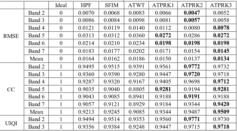
To examine the proposed method for downscaling Landsat 8 images that were acquired long before the Sentinel-2 image, the 90 m Landsat 8 images of 10 April 2015 and 1 November 2014 were downscaled to 30 m. Fig. 6 shows the results for the same 4.5 km by 4.5 km sub-area for the Landsat 8 data of 10 April 2015. Consistent with the observations in the previous two experiments, HPF and SFIM produced speckle artifacts and ambiguous boundaries for changed places, while ATPRK2 cannot provide clear LCLU information at the desired 30 m spatial resolution. The proposed ATPRK3 method can restore most of the boundaries and produced results closest to the reference in Fig. 6(a). The accuracies measured by the six indices in Tables 4 and 5 for the Landsat 8 data of 10 April 2015 and 1 November 2014 (entire 18 km by 18 km study area) also lead to the same conclusion as the visual inspection. More importantly, two further observations can be made from the two tables.
and the Landsat 8 images of 5 August 2015, 10 April 2015 and 1 November 2014 are 13, 125 and 285 days, respectively. Correspondingly, the CCs of ATPRK3 are 0.9560, 0.9527 and 0.9509, respectively.
Second, different from the previous two experiments where the PAN bands were not used for Landsat 8 bands 5-7, in this experiment, the PAN band was used for some of the Landsat 8 bands 5-7 (e.g., bands 6 and 7 of the Landsat 8 data of 10 April 2015). The reason is that as the time interval between the Sentinel-2 image and the Landsat 8 image increases, the changes between the two types of data increase. As a result, the correlation between the Sentinel-2 bands 8, 11 and 12 and Landsat 8 bands 5-7 decreases to be smaller than that between the Landsat 8 PAN and Landsat 8 bands 5-7, and the Landsat 8 PAN band needs to be incorporated into the fusion process to provide more reliable information.
(a) (b) (c)
(d) (e) (f)
[image:14.612.85.530.189.665.2](g) (h) (i)
produced by fusing the 90 m Landsat image with the 45 m PAN image (ATPRK2). (i) ATPRK result produced by fusing the 90 m Landsat image with the 30 m Sentinel-2 and 45 m PAN images (ATPRK3).
Table 4 Quantitative assessment of the downscaling methods for the entire Landsat 8 image of 10 April 2015 (ATPRK1 uses only the 30 m Sentinel-2 data, ATPRK2 uses only the 45 m PAN band, and ATPRK3 uses both
the 30 m Sentinel-2 and 45 m PAN data; the bold values indicate the most accurate result in each term) Ideal HPF SFIM ATWT ATPRK1 ATPRK2 ATPRK3
RMSE
Band 2 0 0.0072 0.0071 0.0077 0.0066 0.0050 0.0051 Band 3 0 0.0094 0.0092 0.0100 0.0087 0.0064 0.0063
Band 4 0 0.0139 0.0136 0.0152 0.0126 0.0090 0.0089
Band 5 0 0.0318 0.0315 0.0370 0.0266 0.0277 0.0266
Band 6 0 0.0225 0.0220 0.0250 0.0207 0.0196 0.0185
Band 7 0 0.0217 0.0211 0.0244 0.0200 0.0176 0.0170
Mean 0 0.0178 0.0174 0.0199 0.0159 0.0142 0.0137
CC
Band 2 1 0.9365 0.9385 0.9340 0.9469 0.9701 0.9693 Band 3 1 0.9245 0.9284 0.9232 0.9379 0.9663 0.9679
Band 4 1 0.9176 0.9210 0.9098 0.9335 0.9662 0.9674
Band 5 1 0.9039 0.9055 0.8786 0.9333 0.9274 0.9333
Band 6 1 0.9030 0.9081 0.8876 0.9183 0.9274 0.9350
Band 7 1 0.9054 0.9114 0.8883 0.9208 0.9392 0.9433
Mean 1 0.9152 0.9188 0.9036 0.9318 0.9494 0.9527
UIQI
Band 2 1 0.9352 0.9373 0.9324 0.9469 0.9697 0.9692 Band 3 1 0.9221 0.9262 0.9220 0.9378 0.9655 0.9679
Band 4 1 0.9148 0.9184 0.9090 0.9330 0.9654 0.9674
Band 5 1 0.9016 0.9033 0.8783 0.9321 0.9247 0.9321
Band 6 1 0.8950 0.9001 0.8875 0.9154 0.9235 0.9325
Band 7 1 0.8989 0.9050 0.8882 0.9186 0.9370 0.9424
Mean 1 0.9113 0.9150 0.9029 0.9306 0.9476 0.9519
ERGAS 0 4.0360 3.9461 4.4960 3.6513 3.1477 3.0496
SAM(°) 0 0.0832 0.0811 0.1038 0.0747 0.0652 0.0648
[image:15.612.106.510.519.742.2]Coherence 1 0.9931 0.9935 0.9743 1 1 1
Table 5 Quantitative assessment of the downscaling methods for the entire Landsat 8 image of 1 November 2014 (ATPRK1 uses only the 30 m Sentinel-2 data, ATPRK2 uses only the 45 m PAN band, and ATPRK3 uses both the 30 m Sentinel-2 and 45 m PAN data; the bold values indicate the most accurate result in each
term)
Ideal HPF SFIM ATWT ATPRK1 ATPRK2 ATPRK3
RMSE
Band 2 0 0.0070 0.0068 0.0083 0.0066 0.0047 0.0052 Band 3 0 0.0086 0.0084 0.0098 0.0081 0.0057 0.0058 Band 4 0 0.0121 0.0119 0.0140 0.0112 0.0080 0.0078
Band 5 0 0.0313 0.0312 0.0360 0.0272 0.0286 0.0272
Band 6 0 0.0214 0.0210 0.0234 0.0198 0.0198 0.0198
Band 7 0 0.0183 0.0177 0.0202 0.0171 0.0154 0.0145
Mean 0 0.0164 0.0162 0.0186 0.0150 0.0137 0.0134
CC
Band 2 1 0.9495 0.9515 0.9391 0.9561 0.9772 0.9732 Band 3 1 0.9360 0.9390 0.9280 0.9447 0.9720 0.9718 Band 4 1 0.9287 0.9320 0.9167 0.9405 0.9698 0.9712
Band 5 1 0.9035 0.9040 0.8805 0.9281 0.9194 0.9281
Band 6 1 0.9043 0.9085 0.8941 0.9188 0.9191 0.9188 Band 7 1 0.9057 0.9121 0.8929 0.9184 0.9344 0.9420
Mean 1 0.9213 0.9245 0.9085 0.9344 0.9487 0.9509
Band 4 1 0.9278 0.9309 0.9145 0.9404 0.9692 0.9712
Band 5 1 0.9005 0.9012 0.8803 0.9269 0.9162 0.9269
Band 6 1 0.8968 0.9005 0.8938 0.9164 0.9141 0.9164
Band 7 1 0.9001 0.9059 0.8926 0.9168 0.9311 0.9402
Mean 1 0.9184 0.9214 0.9069 0.9335 0.9465 0.9499
ERGAS 0 4.1011 4.0103 4.6189 3.7778 3.3606 3.2558
SAM(°) 0 0.0766 0.0754 0.0956 0.0695 0.0677 0.0688
Coherence 1 0.9940 0.9942 0.9749 1 1 1
3.5 Use of the Landsat 8 PAN image in downscaling Landsat 8 bands 5-7
[image:16.612.102.513.49.156.2]The proposed approach determines whether the PAN band should be incorporated into the downscaling of Landsat 8 bands 5-7 according to the correlation between them. This necessitates a comparison between the proposed method (ATPRK3) and the method that uses consistently the PAN band for all Landsat 8 bands 5-7. Fig. 7 shows the results of bands 5-7 for the 4.5 km by 4.5 km sub-area of the Landsat 8 images on 5 August 2015 and 1 November 2014. It is observed clearly that when using the PAN band for all three Landsat bands, the results are ambiguous and some linear features cannot be restored. The results of the proposed approach are visually more satisfactory. The quantitative assessment (in terms of CC) of the two schemes for all four full Landsat 8 observations in Fig. 2(b)-(e) is displayed in Table 6. Although the proposed selective approach sometimes produced smaller CCs for several bands, the CCs for most of the bands as well as the overall accuracies are greater. This experiment validates the rationale of the selective scheme for downscaling Landsat 8 bands 5-7 in the proposed fusion approach.
(a) (b) (c)
(d) (e) (f)
[image:16.612.86.528.363.674.2]bands 5-7. (c) and (f) are ATPRK results produced by fusing the 90 m Landsat image with the 30 m Sentinel-2 and 45 m PAN images using the proposed selective approach.
Table 6 Quantitative assessment (in terms of CC) of the two schemes for downscaling the Landsat 8 bands 5-7 on 5 August 2015 and 1 November 2014 (“All” means considering the PAN band for all bands 5-7, while “Selective” means the proposed selective approach, that is, APTRK3; Y means the PAN band is used for the
Landsat 8 band, while N means not; the bold values indicate the most accurate result in each term) 6 September 2015 5 August 2015 10 April 2015 1 November 2014
All Selective All Selective All Selective All Selective Band 5 0.9178 0.9532 (N) 0.9084 0.9479 (N) 0.9294 0.9333 (N) 0.9220 0.9281 (N) Band 6 0.9347 0.9445 (N) 0.9371 0.9434 (N) 0.9350 0.9350 (Y) 0.9289 0.9188 (N) Band 7 0.9498 0.9480 (N) 0.9471 0.9450 (N) 0.9433 0.9433 (Y) 0.9420 0.9420 (Y)
Mean 0.9341 0.9486 0.9309 0.9454 0.9359 0.9372 0.9310 0.9296 3.6 Results of the 10 m downscaled Landsat 8 images
To reveal the applicability of the proposed fusion approach in practice, we applied it to downscale the observed 30 m Landsat 8 images to 10 m, using the 10 m Sentinel-2 and 15 m PAN images. The results for two Landsat images on 5 August 2015 and 6 September 2015 are shown in Fig. 8. Fig. 9 exhibits the results for the 4.5 km by 4.5 km sub-area, where the results of the method using only the Sentinel-2 information is also provided for visual comparison. The benefits of downscaling are very clear when comparing the 10 m results to the original 30 m Landsat 8 images. For example, the roads, textures of urban fabric and “white” buildings in the 10 m results are obviously much clearer than those in the original 30 m observations. Furthermore, the inter-comparison between the two downscaling approaches (i.e., ATPRK1 and ATPRK3) suggests that by using the 15 m PAN bands, the proposed ATPRK3 approach can produce more satisfactory predictions where more elongated features are present and pixels of LCLU changes are more accurately restored.
(a) (b)
Fig. 8 10 m Downscaling results of the proposed method for Landsat 8 images on (a) 5 August 2015 and (b) 6 September 2015 (bands 432 as RGB).
[image:17.612.97.521.418.638.2](b) (c) (d)
[image:18.612.70.545.50.544.2](e) (f) (g)
Fig. 9 10 m Downscaling results for a sub-area of the Landsat 8 image on 5 August 2015 and 6 September 2015 (bands 432 as RGB). (a) 10 m Sentinel-2 image on 18 August 2015. (b)-(d) are 10 m results for the Landsat image on 5 August 2015, and (e)-(g) are 10 m results for the Landsat image on 6 September 2015. (b) and (e) are the original 30 m Landsat 8 images. (c) and (f) are 10 m ATPRK results produced by fusing the 30 m Landsat images with the 10 m Sentinel-2 images (ATPRK1). (d) and (g) are 10 m ATPRK results produced by fusing the 30 m Landsat images with the 10 m Sentinel-2 and 15 m PAN images (ATPRK3).
4. Discussion
4.1 Contributions
downscaled to 10 m to match that of the Sentinel-2 images. The contributions of this paper lie in the theoretical innovation, technological advancement and application potential.
Theoretically, for each 30 m Landsat 8 band, we borrow the information from the 10 m Sentinel-2 band with the same wavelength and incorporate it into the downscaling process. We also consider the LCLU changes between the Landsat 8 and Sentinel-2 images to increase the accuracy of the downscaled Landsat 8 images. The objective is to take full advantage of all the information provided by the two types of sensors. Technologically, the advanced ATPRK approach is proposed for the fusion task, where the 10 m Sentinel-2 images are treated as covariates and provide valuable fine spatial resolution information. Based on ATPRK, the spectral properties of the original Landsat data can be perfectly preserved. To account for the LCLU changes, a Landsat 8 PAN image is incorporated into the downscaling process for further enhancement. Since the PAN band is always acquired at exactly the same time as the multispectral bands, it encompasses information on changes that cannot be observed by the Sentinel-2 images.
Fusion of Landsat 8 and Sentinel-2 has great potential application value. First, for the Landsat 8 data acquired after the launch date of the Sentinel-2 satellite, they can be downscaled to 10 m and embedded to the available Sentinel-2 time-series data to produce finer temporal resolution data at 10 m spatial resolution, and more continuous global monitoring can be achieved to observe rapid changes on the Earth’s surface. The experimental results in Sections 3.1 and 3.3 where the Landsat 8 data were acquired temporally close to the Sentinel-2 data suggested that the proposed ATPRK-based fusion approach is suitable for coordinating the spatial resolutions of the two types of data for more continuous monitoring. Timely monitoring is critical in a wide range of applications, such as the urbanization process in highly developed cities [4], [5] and deforestation and forest degradation processes (for example in the Amazon rainforest where intervention is needed quickly following the detection of deforestation) [6]. Apart from LCLU changes, the finer temporal resolution Sentinel-2 data will also have great potential in monitoring rapid changes in vegetation phenology, especially in agricultural areas.
Second, the historical Landsat 8 data acquired between February 2013 (the launch time of Landsat 8) and June 2015 (the launch time of Sentinel-2) can also be downscaled to 10 m with the proposed fusion approach. The 10 m products may provide analysts with more explicit LCLU information in these two years than the original 30 m Landsat data. The experimental results in Section 3.4 where the two Landsat 8 datasets were acquired long before the Sentinel-2 data (with time intervals of 125 and 285 days, respectively) revealed that the proposed fusion approach has potential for downscaling historical Landsat 8 data to 10 m.
4.2 Comparison with fusion of Landsat and MODIS data
Fusion of Landsat and MODIS images is an existing solution to provide more frequent fine spatial resolution data for global monitoring, which can synthesize 30 m Landsat-like data at the temporal resolution of the available MODIS data. However, it is substantially different from the fusion problem presented in this paper. The essence of fusing Landsat with Sentinel-2 data is to downscale the 30 m Landsat data to the 10 m Sentinel-2 resolution, while fusing Landsat with MODIS data means downscaling the 500 m MODIS data to the 30 m Landsat resolution. The former involves a zoom factor of only three, but the latter involves a very large zoom factor of 16 and large uncertainties. Moreover, since Landsat and Sentinel-2 data are provided in the same geographic coordinate system (the UTM/WGS84 projection), the geometric registration is more convenient for fusion of the two types of data.
days to five days [42]. Therefore, by fusing Landsat 8 with Sentinel-2 data, up to eight (three for current Sentinel-2A, three for the forthcoming Sentinel-2B and two for Landsat 8) observations can be made per month. Moreover, it would be promising to further consider embedding the 30 m Landsat-like data derived from fusion of Landsat and MODIS data to the coordinated continuous Sentinel-2A, Sentinel-2B and Landsat 8 observations, to provide as frequent data as possible for near real-time global monitoring. Considering the large uncertainties in fusing Landsat and MODIS data, this potential scheme might require pre-processing steps to select out reliable 30 m Landsat-like data in advance.
4.3 Comparison with fusion of Landsat and SPOT data
In some studies, Landsat data were fused with SPOT data to obtain finer spatial resolution Landsat data [43], [44]. This means fusing Landsat multispectral bands with either the SPOT PAN band (e.g., fusion of 30 m Landsat 5 multispectral and 10 m SPOT 4 PAN bands) [43] or SPOT multispectral bands (e.g., fusion of 30 m Landsat 5 multispectral and 10 m SPOT 5 multispectral bands) [44]. This may also be a feasible solution for more frequent monitoring at the global scale. However, SPOT is a commercial satellite imaging mission and the real-time data are generally not freely available. This is not the case for Sentinel-2 data which are available free. If 10 m SPOT 5 data is available, they could be readily considered for incorporation with Sentinel-2 data to downscale the 30 m Landsat 8 data to 10 m, but more importantly, provide more dense real 10 m observations. Recently, the French government space agency opened publicly the SPOT data archive for over five years. This will certainly motivate future research for fusion of Landsat, Sentinel-2 and SPOT data for more continuous monitoring.
4.4 Multiple Sentinel-2 images
In this paper, we consider only one Sentinel-2 image for downscaling Landsat 8 images covering the same area. Based on the ATPRK approach, Sentinel-2 bands are considered as covariates. It would be interesting to use multiple Sentinel-2 images for the fusion problem, on the condition that they are acquired temporally close to the Landsat data of interest. This will become more realistic after the launch of the Sentinel-2B satellite in mid-2016, when the temporal resolution of the Sentinel-2 observations will be increased to five days and more Sentinel-2 images can be included in downscaling Landsat 8 data. Technologically, using multiple Sentinel-2 images is convenient for ATPRK, as the geostatistical approach can readily incorporate multiple covariates by multiple regression.
4.5 Fusion of Landsat 7 and Sentinel-2 images
This paper considers the fusion of Sentinel-2 data with Landsat 8 data. Landsat 7 ETM+ is another sensor in regular operation, but the SLC-off issue hampers its application to some extent. Some approaches have been developed to fill gaps in the Landsat 7 SLC-off images, such as the fundamental localized linear histogram match provided by USGS [45]. When filling SLC gaps, auxiliary full images covering the same area, but acquired at a proximate time, are generally required to provide reference data for the gaps. For example, Landsat 7 SLC gaps can be filled by referring to the Landsat 8 data acquired on proximate days. The gap-filled Landsat 7 data then may be fused with Sentinel-2 data for more continuous monitoring.
of Landsat 7 and Sentinel-2 data. Therefore, in future research it would be worthwhile to develop a more powerful SLC gap-filling procedure and corresponding fusion approaches for combining Landsat 7 with Sentinel-2 data and to study the effect of the PAN band in sharpening the near-infrared band.
4.6 Alternatives for ATPRK
In the proposed fusion approach, ATPRK was used for image sharpening. The experimental results demonstrated consistently that using only the Sentinel-2 image, ATPRK outperforms HPF, SFIM and ATWT. This justifies the use of ATPRK for further incorporating the Landsat 8 PAN band in downscaling Landsat 8 bands 2-7 in the proposed approach. The PAN and Sentinel-2 bands are not fused with the Landsat 8 multispectral bands simultaneously. Specifically, the PAN band is incorporated first and then the Sentinel-2 bands. Because the spatial resolution ratio between the 15 m PAN and 10 m Sentinel-2 bands is not an integer, additional procedures are involved (i.e., steps 3 and 5 in Section 2.2). It would be interesting to develop a one-stage approach that can incorporate the PAN and Sentinel-2 bands simultaneously. Downscaling cokriging may be an appropriate solution to this requirement [32]-[34]. However, this geostatistical solution involves complex cross-semivariogram modeling and the size of the cokriging matrix would be large if both PAN and Sentinel-2 bands are considered.
5. Conclusion
This paper presents a new approach for coordinating the spatial resolutions of 30 m Landsat 8 and 10 m Sentinel-2 data for continuous monitoring. The ATPRK approach was proposed to downscale the 30 m Landsat 8 data to 10 m, treating the 10 m Sentinel-2 bands and 15 m Landsat 8 PAN band as covariates. The proposed fusion approach accounts for the LCLU changes that have occurred between the Landsat 8 and Sentinel-2 image acquisitions. In experiments, we compared the proposed approach with HPF, SFIM, ATWT and another two ATPRK-based approaches that used only Sentinel-2 data and only Landsat 8 PAN data for fusion. The findings from both visual and quantitative evaluation are summarized as follows.
1) ATPRK is more accurate than the HPF, SFIM and ATWT methods, whether or not the Landsat 8 PAN is incorporated in the fusion process.
2) With the aid of the PAN band, ATPRK can satisfactorily account for LCLU changes and produces more accurate downscaling results than the ATPRK approach using only the Sentinel-2 data or only the Landsat 8 PAN band for fusion.
3) ATPRK can perfectly preserve the spectral properties of the original Landsat 8 data.
4) The PAN band may not be useful for downscaling some bands of Landsat 8 bands 5-7, but its value may increase as the LCLU changes between the Sentinel-2 and Landsat 8 data acquisitions increase.
References
[1] T. Arvidson, S. Goward, J. Gasch, and D. Williams, “Landsat-7 long-term acquisition plan: Development and validation,” Photogrammetric Engineering and Remote Sensing, vol. 72, pp. 1137–1146, 2006. [2] D. P. Roy et al., “Landsat-8: Science and product vision for terrestrial global change research,” Remote
Sensing, vol. 145, pp. 154–172, 2014.
[3] F. Gao, T. Hilker, X. Zhu, M. Anderson, J. G. Masek, P. Wang, and Y. Yang, “Fusing Landsat and MODIS data for vegetation monitoring,” IEEE Geoscience and Remote Sensing Magazine, vol. 3, 47–60, 2015. [4] K. C. Seto, “Urban growth in South China: Winners and losers of China’s policy reforms,” Petermanns
[5] M. Castrence, D. H. Nong, C. C. Tran, L. Young, and J. Fox, “Mapping urban transitions using multi-temporal Landsat and DMSP-OLS night-time lights imagery of the red river delta in Vietnam,” Land, vol. 3, pp. 148–166, 2014.
[6] M. C. Hansen, Y. E. Shimabukuro, P. Potapov, and K. Pittman, “Comparing annual MODIS and PRODES forest cover change data for advancing monitoring of Brazilian forest cover,” Remote Sensing of Environment, vol. 112, pp. 3784–3793, 2008.
[7] P. M. Atkinson, C. Jeganathan, J. Dash, and C. Atzberger, “Inter-comparison of four models for smoothing satellite sensor time-series data to estimate vegetation phenology,” Remote Sensing of Environment, vol. 123, pp. 400–417, 2012.
[8] F. Gao, J. Masek, M. Schwaller, and F. Hall, “On the blending of the Landsat and MODIS surface reflectance: Predicting daily Landsat surface reflectance,” IEEE Transactions on Geoscience and Remote Sensing, vol. 44, no. 8, pp. 2207–2218, 2006.
[9] X. Zhu, J. Chen, F. Gao, X. H. Chen, and J. G. Masek, “An enhanced spatial and temporal adaptive reflectance fusion model for complex heterogeneous regions,” Remote Sensing of Environment, vol. 114, no. 11, pp. 2610–2623, 2010.
[10]H. Song and B. Huang, “Spatiotemporal satellite image fusion through one-pair image learning,” IEEE Transactions on Geoscience and Remote Sensing, vol. 51, no. 4, pp. 1883–1896, 2013.
[11]R. Zurita-Milla, G. Kaiser, J. G. P. W. Clevers, W. Schneider, and M. E. Schaepman, “Downscaling time series of MERIS full resolution data to monitor vegetation seasonal dynamics,” Remote Sensing of Environment, vol. 113, pp. 1874–1885, 2009.
[12]T. Hilker, M. A. Wulder, N. C. Coops, J. Linke, J. McDermid, J. G.Masek, F. Gao, and J. C. White, “A new data fusion model for high spatial- and temporal-resolution mapping of forest based on Landsat and MODIS,” Remote Sensing of Environment, vol. 113, no. 8, pp. 1613–1627, 2009.
[13]I. V. Emelyanova, T. R. McVicar, T. G. Van Niel, L. T. Li, A. I.J.M. van Dijk, “Assessing the accuracy of blending Landsat–MODIS surface reflectances in two landscapes with contrasting spatial and temporal dynamics: A framework for algorithm selection,” Remote Sensing of Environment, vol. 133, pp. 193–209, 2013.
[14]M. Drusch et al., “Sentinel-2: ESA’s optical high-resolution mission for GMES operational services,” Remote Sensing of Environment, vol. 120, pp. 25–36, 2012.
[15]O. Hagolle et al., “SPOT-4 (Take 5): Simulation of Sentinel-2 time series on 45 large sites,” Remote Sensing, vol. 7, pp. 12242–12264, 2015.
[16]K. Segl, L. Guanter, F. Gascon, T. Kuester, C. Rogass, and C. Mielke, “S2eteS: An end-to-end modeling tool for the simulation of Sentinel-2 image products,” IEEE Transactions on Geoscience and Remote Sensing, vol. 53, no. 10, pp. 5560–5571, 2015.
[17]Z. Zhu, S. Wang, and C. E. Woodcock, “Improvement and expansion of the Fmask algorithm: cloud, cloud shadow, and snow detection for Landsats 4-7, 8, and Sentinel 2 images,” Remote Sensing of Environment, vol. 159, pp. 269-277, 2015.
[18]T.-M. Tu, S.-C. Su, H.-C. Shyu, and P. S. Huang, “A new look at IHS-like image fusion methods,” Information Fusion, vol. 2, no. 3, pp. 177–186, 2001.
[19]A. R. Gillespie, A. B. Kahle, and R. E. Walker, “Color enhancement of highly correlated images—II. Channel ratio and “Chromaticity” trans-form techniques,” Remote Sensing of Environment, vol. 22, no. 3, pp. 343–365, 1987.
[20]V. K. Shettigara, “A generalized component substitution technique for spatial enhancement of multispectral images using a higher resolution data set,” Photogrammetric Engineering and Remote Sensing, vol. 58, no. 5, pp. 561–567, 1992.
[22]P. S. Chavez Jr., S. C. Sides, and J. A. Anderson, “Comparison of three different methods to merge multiresolution and multispectral data: Landsat TM and SPOT panchromatic,” Photogrammetric Engineering and Remote Sensing, vol. 57, no. 3, pp. 295–303, 1991.
[23]J. G. Liu, “Smoothing filter based intensity modulation: A spectral preserve image fusion technique for improving spatial details,” International Journal of Remote Sensing, vol. 21, no. 18, pp. 3461–3472, 2000. [24]Q. Wei, J. Bioucas-Dias, N. Dobigeon, and J. Tourneret, “Hyperspectral and multispectral image fusion based on a sparse representation,” IEEE Transactions on Geoscience and Remote Sensing, vol. 53, no. 7, pp. 3658–3668, 2015.
[25]C. Pohl and J. L. Van Genderen, “Review article Multisensor image fusion in remote sensing: Concepts, methods and applications,” International Journal of Remote Sensing, vol. 19, no. 5, 823–854, 1998. [26]J. Bioucas-Dias, A. Plaza, G. Camps-Valls, P. Scheunders, N. Nasrabadi, and J. Chanussot,
“Hyperspectral remote sensing data analysis and future challenges,” IEEE Geoscience and Remote Sensing Magazine, vol. 1, no. 2, 2013.
[27]G. Vivone, L. Alparone, J. Chanussot, M. Dalla Mura, A. Garzelli, G. A. Licciardi, R. Restaino, and L. Wald, “A critical comparison among pansharpening algorithms,” IEEE Transactions on Geoscience and Remote Sensing, vol. 53, no. 5, pp. 2565–2586, 2015.
[28]J. Zhang, “Multi-source remote sensing data fusion: status and trends,” International Journal of Image and Data Fusion, vol. 1, no. 1, pp. 5-24, 2010.
[29]Q. Wang, W. Shi, P. M. Atkinson, and Y. Zhao. “Downscaling MODIS images with area-to-point regression kriging,” Remote Sensing of Environment, vol. 166, pp. 191–204, 2015.
[30]Q. Wang, W. Shi, P. M. Atkinson, and E. Pardo-Iguzquiza. “A new geostatistical solution to remote sensing image downscaling,” IEEE Transactions on Geoscience and Remote Sensing, vol. 2016, no. 54, pp. 386–396, 2016.
[31]M. H. R. Sales, C. M. Souza, Jr., and P. C. Kyriakidis, “Fusion of MODIS images using kriging with external drift,” IEEE Transactions on Geoscience and Remote Sensing, vol. 51, no. 4, pp. 2250–2259, 2013.
[32]E. Pardo-Igúzquiza, M. Chica-Olmo, and P. M. Atkinson, “Downscaling cokriging for image sharpening,” Remote Sensing of Environment, vol. 102, no. 2, pp. 86–98, 2006.
[33]E. Pardo-Iguzquiza, V. F. Rodríguez-Galiano, M. Chica-Olmo, and P. M. Atkinson, “Image fusion by spatially adaptive filtering using downscaling cokriging,” ISPRS Journal of Photogrammetry and Remote Sensing, vol. 66, no. 3, pp. 337–346, 2011.
[34]P. M. Atkinson, E. Pardo-Igúzquiza, and M. Chica-Olmo, “Downscaling cokriging for super-resolution mapping of continua in remotely sensed images,” IEEE Transactions on Geoscience and Remote Sensing, vol. 46, no. 2, pp. 573–580, 2008.
[35]P. Kyriakidis and E.-H. Yoo, “Geostatistical prediction and simulation of point values from areal data,” Geographical Analysis, vol. 37, no. 2, pp. 124–151, 2005.
[36]P. C. Kyriakidis, “A geostatistical framework for area-to-point spatial interpolation,” Geographical Analysis, vol. 36, no. 3, pp. 259–289, 2004.
[37]P. Kitanidis, “Generalized covariance functions in estimation,” Mathematical Geology, vol. 25, pp. 525– 540, 1994.
[38]USGS (2015). Using the USGS Landsat 8 Product. Available online at http://landsat.usgs.gov/Landsat8_Using_Product.php.
[39]P. M. Atkinson, “Issues of uncertainty in super-resolution mapping and their implications for the design of an inter-comparison study,” International Journal of Remote Sensing, vol. 30, no. 20, pp. 5293–5308, 2009.
[40]Z. Wang and A. C. Bovik, “A universal image quality index,” IEEE Signal Processing Letters, vol. 9, no. 3, pp. 81–84, 2002.
[42]ESA (2016). Sentinel-2: Operations. Available online athttp://www.esa.int/Our_Activities/Operations/Sentinel-2_operations/(print).
[43]J. Zhou, D. L. Civco, and J. A. Silander, “A wavelet transform method to merge Landsat TM and SPOT panchromatic data,” International Journal of Remote Sensing, vol. 19, no. 4, pp. 743–757, 1998.
[44]H. Song, B. Huang, Q. Liu, and K. Zhang, “Improving the spatial resolution of Landsat TM/ETM+ through fusion with SPOT5 images via learning-based super-resolution,” IEEE Transactions on Geoscience and Remote Sensing, vol. 53, no. 3, pp. 1195–1204, 2015.