warwick.ac.uk/lib-publications
Manuscript version: Author’s Accepted Manuscript
The version presented in WRAP is the author’s accepted manuscript and may differ from the
published version or Version of Record.
Persistent WRAP URL:
http://wrap.warwick.ac.uk/115828
How to cite:
Please refer to published version for the most recent bibliographic citation information.
If a published version is known of, the repository item page linked to above, will contain
details on accessing it.
Copyright and reuse:
The Warwick Research Archive Portal (WRAP) makes this work by researchers of the
University of Warwick available open access under the following conditions.
Copyright © and all moral rights to the version of the paper presented here belong to the
individual author(s) and/or other copyright owners. To the extent reasonable and
practicable the material made available in WRAP has been checked for eligibility before
being made available.
Copies of full items can be used for personal research or study, educational, or not-for-profit
purposes without prior permission or charge. Provided that the authors, title and full
bibliographic details are credited, a hyperlink and/or URL is given for the original metadata
page and the content is not changed in any way.
Publisher’s statement:
Please refer to the repository item page, publisher’s statement section, for further
information.
1Abstract—In this paper, a hydrostatic tidal turbine (HTT) is designed and modelled, which uses more reliable hydrostatic transmission to replace existing fixed ratio gearbox transmission. The HTT dynamic model is derived by integrating governing equations of all the components of the hydraulic machine. A nonlinear observer is proposed to predict the turbine torque and tidal speeds in real time based on extreme learning machine (ELM). A sensor-less double integral sliding mode controller is then designed for the HTT to achieve the maximum power extraction in the presence of large parametric uncertainties and nonlinearities. Simscape design experiments are conducted to verify the proposed design, model and control system, which show that the proposed control system can efficiently achieve the maximum power extraction and has much better performance than conventional control. Unlike the existing works on ELM, the weights and biases in the ELM are updated online continuously. Furthermore, the overall stability of the controlled HTT system including the ELM is proved and the selection criteria for ELM learning rates is derived. The proposed sensor-less control system has prominent advantages in robustness and accuracy, and is also easy to implement in practice.
Index Terms—Tidal turbine; Hydrostatic transmission; Extreme learning machine; Sensor-less control; Double integral sliding control.
I. INTRODUCTION
IDAL currents are becoming an increasingly favorable alternative to conventional energy sources and have the potential to play a valuable role in the future renewable energy generations. The potential of sustainable electrical power generation from tidal currents provides a promising, clean and reliable solution to the huge and ever-increasing demand of modern society. The harnessing of tidal energy requires the conversion of kinetic energy from free flowing tidal currents into a mechanical turbine system which then drives the generator to produce electricity. Tidal turbines are in principle very similar to wind turbines but work in harsh and deep seawater conditions. The main differences are that a tidal turbine is much smaller and spins more slowly than a wind turbine of equivalent power rating, but generates a much larger thrust and predictable power due to the much higher density of the seawater (more than 800 times denser than air) and the predictable features of tidal currents [1]. In addition, the enormous tidal energy generation directly exploits tidal current speeds without requiring large civil engineering structures to build up a water head like a dam.
Tidal turbine technology is still in its infancy. Like wind
1X. Yin and X. Zhao (corresponding author) are with the School of Engineering, University of Warwick, Coventry, CV4 7AL, U. K. (email: [email protected], [email protected]). This work was
turbines, the horizontal-axis tidal turbines constitute the majority of currently available tidal turbines [2]. Recently, the interest has been growing in the demonstration projects of tidal power. A Seaflow horizontal-axis turbine has been developed and installed in North Devon, UK through the marine current turbine (MCT) project [3]. It is rated at 300 kW and has a rotor speed of 15 rpm and a shaft diameter of 2.1 m. MCT’s second project, the Seagen turbine was designed to produce three times the power of Seaflow. Each rotor of Seagen turbine drives a powertrain consisting of a gearbox and a generator rated at around 500 kW. Hammerfest Strøm developed a 300 kW tidal current turbine with blades of 15-16 m [4]. This turbine is able to operate in both tidal directions by using pitch control. Other demonstration projects include the SMD Hydrovision TidEL Project (UK) [5], the Lunar Energy Project (UK) [6], the HydroHelix Energies Project (France) [7], the free flow turbine project developed by Verdant Power Ltd based in the USA and Canada [8]. However, all these demonstration turbines are equipped with speed-increasing mechanical gearboxes. The increased gearbox ratio may require multiple gearbox stages that increase complexity and failure rates. The continuous operations in harsh and highly turbulent working conditions will pose significant challenges with regards to the survivability of these gearboxes that have the longest downtime and the highest maintenance cost among various tidal turbine failure modes [9].
As an alternative, hydrostatic power transmission may provide a more feasible option for a more reliable tidal power production. A hydrostatic tidal turbine (HTT) is constructed by replacing the fixed ratio mechanical gearbox with a hydrostatic power transmission, like the hydrostatic wind turbine (HWT) [10]. The HTT offers fast response and high reliability, and allows continuously variable speed operations. It is capable of maintaining high overall efficiency. The hydrostatic transmission decouples the tidal turbine from the generator, protecting the turbine system from dangerous situations like over-loading or blade failures. In addition, the HTT allows for more modular and flexible layouts. At the moment, there are very limited studies on the HTT concept in the literature. In [11], the feasibility of applying a hydraulic transmission (based
on Digital DisplacementTM technology) in a tidal current
generator was studied. The aim was to investigate the ability of the hydraulic system in coping with short-term stream velocity variations. Its focus was on the hydraulic transmission while the other aspects were not presented in details. The feasibility for
supported by the UK Engineering and Physical Sciences Research Council under grant EP/R007470/1.
Sensor-less Maximum Power Extraction Control
of a Hydrostatic Tidal Turbine Based on
Adaptive Extreme Learning Machine
Xiuxing Yin and Xiaowei Zhao
using hydraulic transmission in developing special low speed directly driven tidal turbines were studied in [12]. In [13], a HTT was adopted to stabilize the generator power output and optimize power capture. A case study based on a 20 kW horizontal axis HTT was undertaken. However, this work does not focus on control aspects.
Due to the technological similarities between HTTs and HWTs, the control and optimization methodology acquired from HWTs e.g., in [14], [15], may be transferred to accelerate the development of HTT technologies. However, there are some fundamental differences in the design and operation between HWTs and HTTs. Unlike HWTs, the rotor of a HTT runs at low rotational speeds and generates correspondingly high levels of torque and power than a HWT with the same rotor size because of the significantly higher density of seawater over air. In addition, the HTTs are subject to relatively very high variations of rotor speed and turbine loads than HWTs of the same power rating. Furthermore HTTs are submerged systems and they have to withstand harsh submerged conditions, such as marine current turbulences and biofouling. All of these pose extra challenges in the control techniques of HTTs.
In order to achieve the maximum power point tracking (MPPT) and guarantee high operation efficiency of the tidal turbines, there is a need for a highly efficient control design. We are not aware of any such literature for HTT. Even in the context of the conventional gearbox based tidal turbines, relatively few works have focused on the MPPT control of tidal turbines. A proportional-integral-derivative (PID) controller was designed in [16] to maximize the power output of a mechanical gearbox based tidal turbine by varying the rotor speed to maintain the optimum tip speed ratio. Whitby et al. developed a linear MPPT controller for a pitch and a stall regulated horizontal variable-speed tidal turbine [20]. Sliding mode control has been proposed in [17] and [18] to increase tidal power generation efficiency. Zhou et al. dealt with power control strategies for a fixed-pitch direct-drive tidal turbine [19]. A flux-weakening strategy and a torque-based control with feedback flux-weakening strategy were then investigated to realize appropriate power control. However these works did not consider system nonlinearities and uncertainties which are important for tidal turbines in harsh tidal conditions.
This paper aims to investigate the design, modelling and sensor-less optimal power extraction control for a 150 kW HTT under time-varying tidal speed conditions. The HTT is designed by coupling a horizontal-axis tidal turbine rotor with a hydrostatic transmission that consists of variable displacement hydraulic machines. The HTT dynamics is modelled by combining the governing equations of the turbine components. An extreme learning machine (ELM) based nonlinear observer is proposed to achieve sensor-less observations of tidal stream speeds and turbine torque. The ELM is a neural network based learning algorithm which aims to efficiently deal with both single-hidden-layer feedforward networks and multi-hidden-layer feedforward networks [21]. Different from traditional learning algorithms, the ELM not only has better universal approximation capability but also has faster learning speed [22]. The conventional ELM achieves the learning capability by
randomly generating weights and biases in hidden neurons. Following the design of the ELM based nonlinear observer, a double integral sliding controller is constructed to maintain the optimal turbine speed and hence to achieve the maximum tidal power extraction regardless of large parametric uncertainties and external disturbances. Design experiments based on Simulink/Simscape are conducted to verify the proposed design, modelling and the ELM based double integral sliding control algorithm. Significantly different from existing works on ELM and tidal turbine controls, the weights and biases in the employed ELM are updated online continuously for real-time power control of the HTT. In addition, this paper not only proves the stability of the sensor-less control system including the ELM, but also derives the selection criteria for ELM learning rates. Furthermore the proposed sensor-less control has significant advantages in robustness and accuracy, and is easy to implement in practice due to its simplicity and low computational burden.
II. THE HYDROSTATIC TIDAL TURBINE
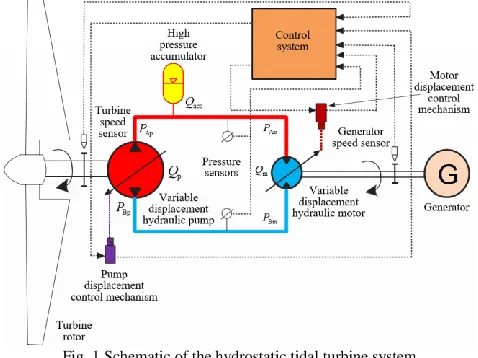
[image:3.612.323.562.431.610.2]As illustrated in Fig. 1, the HTT mainly consists of a turbine rotor, a variable displacement hydraulic pump, a high pressure accumulator, a variable displacement hydraulic motor, an asynchronous squirrel cage induction generator, pump/motor displacement control mechanism and control system. The low speed and variable displacement hydraulic pump is directly driven by the turbine rotor to convert the kinetic input energy into pressurized hydraulic fluid, which then drives the high speed hydraulic motor through hydraulic pipelines. The hydraulic motor is coaxially coupled with the generator which produces electric power.
Fig. 1 Schematic of the hydrostatic tidal turbine system
decoupled dynamics, allowing large power spikes due to tidal gusts and turbulences to be better mitigated and enabling the generator to operate at a constant speed. Therefore, conventional generator side frequency converter can be entirely dispensed in the HTT.
The HTT also allows for multiple-input, single-output tidal turbine configuration in which the hydraulic power generated by multiple individual mechanically coupled turbine rotor and hydraulic pumps are combined to drive a central hydraulic motor/generator unit through a hydraulic pipeline network, allowing for tidal energy collection from multiple turbines. This configuration also allows placing the turbine rotors and hydraulic pumps vertical at the bottom of a tower in the ocean while locating the hydraulic motor/generator unit and additional components on ground level (which are easy to maintain). This will substantially reduce tower mass, and maintenance costs, which stretches the applicability of installing large scale tidal turbines. In addition, other advantages of HTTs over mechanical gearbox based tidal turbines include higher compactness, lighter transmission, faster response, which is attractive for large scale tidal power deployment [23].
III. HTTDYNAMICS MODELLING
The HTT dynamic models are derived by integrating the governing equations of all the turbine components (Fig. 1).
A. Hydrodynamics of the Turbine Rotor
The turbine rotor is featured by its hydrodynamic power/torque-speed characteristics. The tidal power captured by the turbine rotor is given by
3 3 t
t t t p
2
R v
P T C
(1)
where Pt and Tt denote the turbine power and torque inputs,
respectively,
andv
denote seawater density and tidal flowspeed, respectively, R and
t denote the turbine radius androtating speed (also the hydraulic pump speed), respectively,
p
C and are the power capture efficiency coefficient and tip
speed ratio that is a function of tidal stream speed and turbine radius.
t R
v
(2)
The efficiency coefficient Cp depends on the turbine pitch angle and the tip speed ratio and is a monotonic function of the tip speed ratio for the HTT with fixed pitch angle of 0° [24]. Thus,
p
( 0.1)
0.6966sin 0.0037 3 14.94
C
(3)
In practice, the tidal stream speed is measurable and predictable, and is considered to vary between 0 and 3.5 m/s for the HTT. The rated tidal speed is designed as 2 m/s and the power generation under this speed is 150 kW, which suggests the blade radius should be designed as 5 m. The rated turbine speed and torque are respectively 3 rad/s and 50 kNm, which requires a low-speed and high torque hydraulic motor to be
coupled with the tidal turbine.
B. The Hydraulic Pump
Since the hydraulic pump is connected directly to the turbine rotor, the dynamics of the two coupled components is
t p Ap Bp fp t t t
TD P P C J (4)
where PAp and PBp are respectively the inlet and outlet pressures of the hydraulic pump, Cfp and Jt are respectively the friction coefficient and inertia of the two coupled
components, Dp is the pump displacement which can be
continuously varied by using a variable displacement servo control mechanism. The mechanism requires a small electrohydraulic servo for angular positioning and typically consists of an electrohydraulic servo-valve, a piston for actuation, appropriate electrical feedback devices, and electronic error amplifiers [25]. Since the dynamics of servo mechanism is relatively faster than the HTT, it is reasonable to model the mechanism as a proportional element as
p 1 p
D K (5)
where K1 and p are respectively the constant pump
displacement gradient and pump control input.
The pump in–out flowrate Qp is formulated based on
continuity equations [25] as follows
p p t pL Ap Bp
Q D C P P (6)
where CpL is the overall leakage coefficient of the hydraulic pump.
C. The Accumulator
A high-pressure hydraulic accumulator is employed to prevent excessive pressure buildup and hence to maintain a sufficiently high pressure in the suction ports of the hydraulic
machines. Assuming PAp PBp , the flowrate Qacc of the
hydraulic accumulator is written as
Ap acc 1
acc acc
acc Ap acc
Ap
0 if
d
1 if . d
P P
Q P
V P P
t P
(7)
where Vacc and Pacc are respectively the preset volume and
pressure of the hydraulic accumulator,
is a adiabaticcoefficient.
D. The Hydraulic Motor and Pipelines
The in–out flowrate Qm can also be derived by using
continuity equations [26] as follows
o
m m g mL Am Bm Am Bm
e
V
Q D C P P P P
(8)
where PAm and PBm are respectively the inlet and outlet
hydraulic motor and the effective elastic modulus that is a constant 2000 MPa, Dm is the hydraulic motor displacement
that is continuously controllable by using a similar variable displacement servo control mechanism. It is also reasonable to assume a proportional element of the control mechanism due to its relatively faster dynamics compared with the HTT. Thus,
m m m
D K (9)
where Km and m are respectively the constant motor
displacement gradient and hydraulic motor control input. Since the hydraulic motor is rigidly connected to the generator and operates at the same angular speed as the generator, the input torque exerted on the generator shaft is formulated as
m Am Bm g g fg g g
D P P J C T (10)
where Cfg and
J
g are friction coefficient and total inertia of the hydraulic motor driven generator system, respectively, Tg is the reaction torque of the generator.The relationship between the hydraulic pump port pressures and motor chamber pressures can be approximated as
Ap Am pipe Bp Bm pipe
P P P
P P P
(11)
where Ppipe is pressure loss of the pipelines connecting the two hydraulic machines.
Assuming that the in–out flowrate from the hydraulic pump is equal to that of the hydraulic motor,Qp Qm, it is reasonable
to neglect the pipeline pressure drop Ppipe and thus,
Ap Am, Bp Bm
P P P P .
E. The Generator Dynamics
The employed asynchronous induction generator always operates around the synchronous speed of 188 rad/s and offer several advantages including high robustness and low maintenance cost. The generator also has four quadrant active and reactive power capabilities, which lead to lower converter costs and lower power losses. The generator dynamic model is described in the synchronously rotating d/q reference frame with the q-axis aligned with the stator voltage and the stator resistance is neglected [27]. Therefore, the generator dynamics in the d/q reference frame is
2 rd 2
s r r rd r rd s s r r rq
sd
s
rq
2 2
s r r rq r rq s s r r rd
s sd
s
g sd rq
s d 1 1 d d d d 1 1 d . l l l i
M L L L u R i s M L L L i
t M
L t
i
M L L L u R i s M L L L i
t M
s L
M
T p i
L (12)
where i r d, i r q, u r d, u r q denote the d and q-axis rotor currents
and voltages, respectively, R r and L r denote the rotor
resistance and inductance, respectively, L s, M , s d and
p
denote stator inductance, mutual inductance, d-axis stator magnetic flux and pole pair number, respectively, sl and s denote speed slip and synchronous speed of the DFIG, respectively, Tg denotes generator electromagnetic torque.
F. The System Dynamics
The overall dynamics of the HTT can be obtained by combining the above equations from (4) to (10), which can then be described by using a transfer function as follows
2
2 g 1 g 01 g 02 t
g 3 2
3 2 1 0
( ) ( ) ( ) ( )
( )s b T s s b T s s b T s b T s a s a s a s a
(13)
where s is the Laplace operator, and
mL g t pL g t
2
fp pL g p g fg ml t fg pL t
fg fp o 2
m t e
2 2
fg fp mL f t g o 3
e
t fg g fp o 2
e
1
0 g fp pL fp m fg p
;
;
. ;
C J J C J J
C C J D J C C J C C J
C C V D J
C C C C
J J V a
J C J C V
a
a
C
a C C C D D
(14) and t o e f 2 1 01 p 02 o
pL t mL t g
e 2 fp mL fp pl p
m p ; ; ; . J V C V
C J C J T
C C C C D
D b b D b b (15)
As illustrated from (13) to (15), the HTT dynamics can be modelled as high-order ordinary differential transfer function with both the turbine and generator torques as inputs, and the generator speed as output. Since the effective elastic modulus
e
is relatively large (2000 MPa) as compared with Jt, Jg ando
V , it is reasonable to simplify the transfer function (13) as follows
1 g 01 g 02 t
g 2
2 1 0
( ) ( ) ( )
( )s b T s s b T s b T s
a s a s a
(16)
It is obvious from (16) that the hydrostatic transmission functions as a second-order low pass filter without any integrators. Hence, the HTT dynamics can be reliably smoothed and the generator can run at a relatively constant speed regardless of fluctuations of the turbine and generator torques.
IV. MAXIMUM POWER EXTRACTION CONTROL
When the tidal speed is below rated, the HTT seeks to maximize the tidal power generation by maintaining the tip speed ratio at the optimal value opt. As shown in (2) and (4),
it is possible to achieve this target by controlling the hydraulic
pump displacement to keep the speed
t at the optimal valuetopt
partially unknown due to parametric uncertainties and nonlinearities. For instance, the turbine torque input
T
t is generally unknown and uncertain due to the unknown time-varying tidal stream speed. The dynamic model of the HTT is also highly nonlinear and uncertain due to the uncertain leakage, varying oil temperature, variations in control volumes and frictions that cannot be modeled accurately. In addition, there are also un-modeled HTT dynamics and unknown external disturbances. Therefore, in order to achieve the maximum tidal power extraction in the presence of large parametric uncertainties and nonlinearities, a nonlinear observer is proposed herein to observe the turbine torque and tidal speeds in real time based on ELM. Consequently, a double integral sliding mode controller is developed to maintain the optimal turbine speed since the sliding mode control approach is highly efficient and robust in addressing large disturbances and parameter variations of complex nonlinear systems [28].A. ELM Based Nonlinear Observer
A 3-input and 1-output ELM is designed to observe the turbine torque. By multiplying both sides of (4) with
t andusing (1), the following equations are derived
2t t p Ap Bp t fp t t t t 2
p fp t t t t t
t
T D P P C J
P C J
T
(17)
where Pp is the hydraulic pump power that is calculable based
on the product of the pump flowrate and system pressure, Cp
and can be viewed as nonlinear functions of the turbine speed
t under certain tidal speed.As shown in (17), it is natural to approximate the turbine
torque from the hydraulic pump power Pp, pump speed
t, andspeed variations
t by using a 3-input and 1-output ELM. TheELM based observer can achieve sensor-less observations without using expensive physical sensors for measuring tidal stream speeds and turbine torque, thus labelled as "sensor-less" observer. The speed and power of the hydraulic pump are readily measurable with built-in sensors, which are cheaply available as opposed to measurements of the tidal current speed and torque.
As shown in Fig. 2, the employed ELM has a 3-node input layer, an L-node single hidden-layer and a one-node output
layer. Considering N data samples (x, y) with input
T T 31, 2, 3 p, t, t
N
x x x P
x and output 1N
y , the
ELM is mathematically represented as
T
yβ H (18)
where β is the output weight vector, H is the output sigmoid
function matrix [29].
1
1
1 1 1 1
T
1 1
, , , ,
, , , ,
L L
L L
N L L N N L
h b x h b x
h b x h b x
β
ω ω
H
ω ω
(19)
where ωi1 3 and bi are respectively hidden-layer weights and biases, and h
i, ,b xi i
is the sigmoid function.In particular, the turbine torque can be approximated as
*T t
T β H (20)
where is an approximation error, β*Tis the optimal constant
output weight vector.
Given the derived turbine torque in (20), the tidal stream speed is obtained based on (1) and (2). Thus,
1 1
4 4
t t t
2 2
p p
2T 2y
v
R C R C
[image:6.612.316.563.259.449.2] . (21)
Fig. 2 The structure of the employed ELM B. Control Design
By substituting (20) and (5) into (4) and rearranging the resulting equation, one obtains
*T
1 p Ap Bp fp t t
t
K P P C
J
β H (22)
where is lumped uncertainties/uncertain nonlinearities due
to other external disturbances, un-modeled friction forces, and other un-modelled dynamics, and max, where max is the
maximum value of .
By defining the turbine speed tracking error e
topt
t, a double integral sliding surface is defined asi
d
pd
dk
e t k
z
e t k e
(23)where k i, kpand kd are constant control coefficients.
Based on (5) and the sliding surface in (23), the pump control command is designed as
p i d
fp d t t d topt
t t
p
1 d Ap Bp
d sign( )
k e k e t z k
C k
J J y
K P
J k
k P
where is a positive control gain to be specified latter. Instead of using traditional ELM that employs gradient-based learning method and randomly generates hidden-layer weights and biases [30], [31], the weights and biases in this ELM (18) are updated online continuously as follows
1 1 2 3 , , 1, 2,...,i i i i i i
i i i
i i i
b z z
z i L
z
β η H x η β
ω η ω
b η b
(25)
where η η η1, 2, 3L L are constant diagonal learning rate
matrices.
C. Stability Analysis
By utilizing the control command in (24) and the updation law in (25), the closed-loop control system will converge to the sliding surface z in finite time. In order to verify this, a positive definite Lyapunov function candidate is defined as
d
2 T 1 T 1 T 1
1 2 3
t
1 1 1
( ) tr( )
2 2 2 2
V t z
J
k
β η β ω η ω b η b (26)
where * * * 1
, , L
β β β ω ω ω b b b are the
corresponding estimation errors of the weights and biases, ω*
and b* are the optimal constant output weight vector,
hidden-layer weight and bias vectors, respectively, tr( ) denotes the matrix trace of . For brevity, H
i, ,bi x
is denoted as H.Thus, by substituting (24) into the time derivative of (26) and using (22), one obtains
d T T 1
1 t t d t 1 1 3 d T T 2 sign( ) ( ) tr( )
V t z
J J
k
J
k k
z
β H β η β
ω η ω b η b
(27)
Substituting (25) into (27) yields
t
d T T T
t d
( ) sign( ) tr( )
V t z z k k z z z
J J
β β ω ω b b (28)
By using the property of vector norm [32], one obtains
2 2
T T * *
max 2
2 2
max max max
2 2
T T * *
max 2
2 2
max max max
1 1 1 2 4 4 1 1 1 2 4 4
b
b b b
β β β β β β β β β β
β
b b b b b b b b b b
b
(29)
Similarly, due to the property of matrix Frobenius norm [32], one obtains
T
T
*
* 2F F F
2
2 2 2
max max max max
F F F
tr tr
1 1 1
2 4 4
ω ω ω ω ω ω ω ω
ω ω ω
(30)
where max,max,bmax are the maximum values of the norms of the corresponding vectors,
F
ω denotes the Frobenius norm of
ω.
Substituting (29)-(30) into (28) yields
2 2 2
max max ma d t d x t ( ) 4 4 b
V t k k z
J J
. (31)
If the control gain
is selected to satisfy the followinginequality
2 2 2
max max max max
t t d d 4 4 k J J k b
(32)
then, V t( )0. Since V(t) is non-increasing and upper bounded, the designed controller and updation law lead to the closed-loop stable dynamics in which the turbine speed asymptotically converges to the optimal value topt in finite time based on the Barbalat's lemma [33].
D. Selection of Learning Rates
In order to guarantee the convergence of the ELM, the learning rate matrices η η η1, 2, 3 needs to be properly selected.
Hence, a quadratic performance index J k
is defined at timek in the discrete time domain to determine the learning rates.
1 2
2
J k z k . (33)
The time variation of J (k) is
1 2
2
1
2
1 2
2 2
J k z k z k z k z k z k
. (34)
The variations of sliding surface z k
can be expressed in variations of the weights and biases as follows
z z zz k
β β ω ω b b
. (35)
Substituting (25) into (35) gives
1 2 3
T
z z z
z k z k z k z k
z k
η β H η ω η b
β ω b
P ηQ
(36)
where T
T1 2 3
, , , diag , , , , ,
z z z
P η η η η Q β H ω b
β ω b
.
Substituting (36) into (34) gives
22 T 2 T
1 2sign 2
J k z z k z k
P ηQ P ηQ . (37)
To guarantee the convergence of the ELM, we have
0J k
, which requires that the following conditions hold:
1 2 3
1 2 3
1 2 3
2 0, if ( ) 0
, if ( ) 0
0 2, if ( ) 0
z z z
z k
z z z
z k
z z z
z k
η β H η ω η b
β ω b
η β H η ω η b
β ω b
η β H η ω η b
β ω b
(38)
until satisfactory results are obtained.
Significantly different from recent literature on neural network based controls that only consider selections of learning rates and neglect the overall system stability [34], [35], this section not only proves the stability of the overall system including the ELM, but also gives the selection criteria for learning rates.
V. VALIDATIONS AND DISCUSSIONS
The simulation validations of the proposed HTT were conducted by using the credible Simulink/Simscape.
A. Design Experiments
As shown in Fig. 3, the 150 kW HTT Simscape models have been built to conduct the design experiments. The models mainly include a tidal turbine rotor module, ELM, double sliding control, hydrostatic modules and an asynchronous induction generator module.
The tidal turbine rotor module is used to calculate the tidal turbine torque inputs and the optimal turbine speed based on (1)-(3) and by using rotor radius of 5 m and the optimal tip speed ratio opt of 8.
The optimal turbine speed is designed as
opt topt
v R
(39)
The generated turbine torque is set as input for the hydraulic pump via a torque source converter, and the pump speed and its optimal values are fed back into the turbine controller to generate necessary control actions for regulating the pump displacement. The rated operating speed and torque of the hydraulic pump are respectively 3 rad/s and 50 kNm under the tidal stream speed of 2 m/s. Therefore, the rated displacement of the hydraulic pump is calculated as 150 kW/50 MPa/3 rad/s
=0.001 m3/rad. The hydrostatic modules were designed based
on Fig. 1 and include other models such as a replenishing supply, check valves, and a pressure relief valve, pipeline dynamics, flowrate and hydraulic pressure sensors. The setting pressure is kept at 50 MPa by an accumulator. The hydrostatic modules are used to couple the hydraulic motor with the hydraulic pump through necessary pipelines with length of 10 m. Since the hydraulic motor is directly connected with the generator and operates around 189 rad/s, the maximum displacement of the hydraulic motor can be calculated as 150
kW/50 MPa/189 rad/s = 1.6×10⁻⁵ m3/rad. The maximum
pump/motor strokes are 0.005 m and the turbine/generator
inertias are set to be 600 kgm2. The generator is driven by the
hydraulic power that is calculated by using the measured hydraulic pressure and flowrate in the hydrostatic modules. The generator torque and speed are fed back to the hydraulic motor through torque source and angular velocity source so that the hydraulic motor is synchronized with the generator. The generator is modeled by using a WYE-delta starting circuit and runs at the synchronous speed of 189 rad/s, the rated voltage of 440 V, and the rated frequency of 60 Hz. The generator power is optimally captured by torque control through varying the displacement of the hydraulic motor.
Since the generator speed is relatively constant, the optimal torque input for the generator control is derived based on (16).
2
g 2 1 0 02 topt gopt
1 01 5
2 topt 3 popt topt
opt
2
a s a s a b T T
b s b R
T C
(40)
Based on (40), the optimal power control for the hydraulic motor/generator is readily achievable with (40) as reference using a generator side PID controller due to the simple first order hydraulic motor dynamics in (10).
The ELM parameters are calculated and updated online based on (25), and the updated ELM parameters are used as inputs for the ELM module to calculate the turbine torque by using the ELM model in (18). The calculated turbine torque is then fed back into the double sliding turbine controller module to calculate the control signals for the hydraulic pump and estimate the inflow tidal stream speed online by using (21). The proposed turbine controller and ELM model are designed by using MATLAB functions based on the equations in section IV. The proposed controller has also been compared with a conventional PID controller. The key control parameters are
p 3.787
k , ki 1.8 10 3, kd1,
3
1.2 10
, 4
1 m 5 10 m/V
K K ,
L=10.
In order to design the PID controller for comparisons, the model blocks are linearized and a linear analysis is conducted to obtain a linear model in MATLAB. Then, the proportional, integral and derivative parameters of the PID controller are derived based on the linear model by using Ziegler-Nichols tuning method [36].
The ELM training process was conducted by using 106
training samples of realistic tidal pattern before the online implementation of the HTT and controllers. The training of ELM consists of the random mapping and the parameters solving stages. The random mapping stage is used to construct the hidden layer with 10 mapping neurons and randomly generated biases and input weights between -1 and 1, where the mapping is conducted through the sigmoid function. The output weights between hidden neurons and the output nodes, can be
obtained through solving the equation T 1 T
( )
β HH H y , which
can be readily solved by using the MATLAB function pinv. The
obtained ELM parameters are set as the initial values for the online update laws in (25).
The implementation of the HTT also considers the model nonlinearities and uncertainties due to the uncertainties of the damping/friction coefficients, the inertias, and the variations of hydraulic flowrates, and the nonlinearity of the turbine torque and other un-modeled or unknown dynamics. The model uncertainty also includes the mismatch between the HTT model derived in section III and the Simscape model whose source codes are not explicitly obtainable. All of these uncertainties are
lumped into the uncertain term in (22), which can be readily
Fig. 3 The Simscape models of the HTT
B. Results and Discussions
As shown in Fig. 4, the real-world tidal speed varies from 1 m/s to 2 m/s with 5% turbulence intensity, which represents the realistic normal tidal stream conditions. Since the rated tidal speed of the HTT is designed as 2 m/s, the tidal speed sequence in this figure represents the HTT operating conditions when tidal speed is below the rated value. Fig. 4 also shows the tidal speed observer based on ELM and (21) approximates the actual speed very well demonstrating its high effectiveness.
Fig. 4 The tidal turbine speeds
[image:9.612.305.569.59.424.2]As shown in Fig. 5, the observed turbine torque from the ELM agrees well the actual torque generated from actual tidal speed, and thus validates the efficiency of the ELM in observing high-frequency torque fluctuations. As seen from Figs. 4 and 5, sensor-less optimal power control of the HTT is readily achievable without tidal speed and torque sensors.
Fig. 5 The tidal turbine torques
As shown in Fig. 6, tidal turbine speed is better maintained at the optimal values by using the proposed controller, whereas the speed fluctuates significantly when using the conventional controller, particularly between 5.5 s and 10 s when large tidal torque inputs occur. Hence, the proposed controller offer better tracking performance than conventional control.
Fig. 6 The tidal turbine speeds
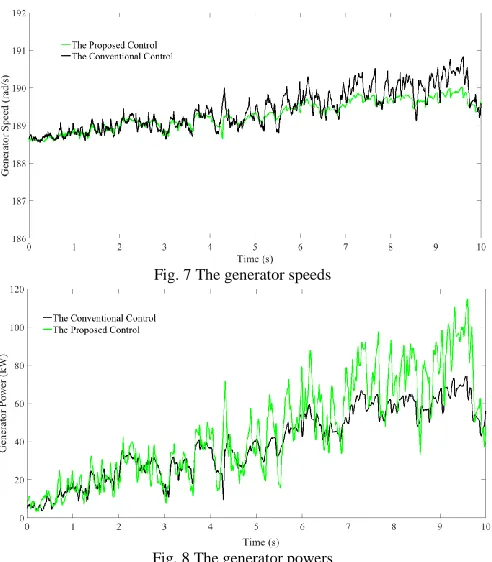
As illustrated in Figs. 7 and 8, the proposed control can better maintain the rated generator speed of 188 rad/s and capture much more generator power due to its intelligent control nature. Thus, the proposed control has much higher effectiveness than the PID control.
0 1 2 3 4 5 6 7 8 9 10
Time (s) 1
1.1 1.2 1.3 1.4 1.5 1.6 1.7 1.8 1.9 2
T
id
al
S
tr
ea
m
S
p
ee
d
(
m
/s
)
[image:9.612.55.301.394.534.2] [image:9.612.318.568.498.634.2]Fig. 7 The generator speeds
Fig. 8 The generator powers
Figs. 9-11 describe the transient behaviors of the ELM parameters including the hidden-layer weights ω10 3 , the biases b10 1 and the output weights β 10 1 . Since the
ELM parameters b and β are all vectors, we use their mean values to represent their dynamic behaviors. For the matrix of
the hidden-layer weights ω10 3 , we use three mean values
1, 2, 3
[image:10.612.319.572.49.326.2]
of the corresponding three columns ofω
to describe the transient behavior of the output weights. A close view to these transient behaviors demonstrates that all the ELM parameters converge to their optimal values quickly and accurately regardless of the model uncertainty and nonlinearity. The accurate convergence can be readily achieved around 0.1 s, which verifies the fast response of the online parameter update laws in section IV-B. Moreover, the convergent values of the ELM parameters can be maintained highly stable despite some very slight drifts due to the variations of the double integral sliding surface z in (23), which further demonstrates the stability of the overall system.Fig. 9 The time evolution of the hidden-layer weights
Fig. 10 The time evolution of the biases
Fig. 11 The time evolution of the output weights
VI. CONCLUSION
This paper has presented the design, modelling and sensor-less optimal tidal power extraction control of a 150 kW HTT. The modelling of the HTT takes into account system nonlinearities and parametric uncertainties associated with hydrostatic dynamics. An ELM based nonlinear observer has been designed to achieve sensor-less observations of tidal stream speeds and turbine torque. Based on the observed parameters, a double integral sliding controller has been proposed for the optimal tidal power extraction. The proposed design, modelling and control of the HTT have been validated by simulations using the credible Simulink/Simscape, which showed that the proposed control systems achieved much better performance than PID control. The design experiments have provided an in-depth insight into the HTT performance evaluations. Further work will focus on the deployment of the sensor-less optimal power control to other experimental platforms including hardware-in-the-loop systems.
REFERENCES
[1] Ouro P, Harrold M, Stoesser T, et al. Hydrodynamic loadings on a horizontal axis tidal turbine prototype. Journal of Fluids and Structures, 2017, 71: 78-95.
[2]https://www.worldenergy.org/wp-content/uploads/2017/03/WEResources_Marine_2016.pdf [3] http://www.marineturbines.com/home.htm
[4]
http://www.aquaret.com/images/stories/aquaret/pdf/cstshammerfeststrm.pdf [5] http://www.reuk.co.uk/wordpress/tidal/tidel-tidal-turbines/
[6] http://www.reuk.co.uk/wordpress/tidal/lunar-energy-tidal-power/ [7] https://hal.archives-ouvertes.fr/hal-00531255/document [8] https://www.verdantpower.com/
[image:10.612.52.575.559.717.2][10] Pedersen N H, Johansen P, Andersen T O. Optimal control of a wind turbine with digital fluid power transmission. Nonlinear Dynamics, 2018, 91(1): 591-607.
[11] Payne G S, Kiprakis A E, Ehsan M, et al. Efficiency and dynamic performance of Digital Displacement™ hydraulic transmission in tidal current energy converters. Proceedings of the Institution of Mechanical Engineers, Part A: Journal of Power and Energy, 2007, 221(2): 207-218. [12] Fraenkel P L. Power from marine currents. Proceedings of the Institution
of Mechanical Engineers, Part A: Journal of Power and Energy, 2002, 216(1): 1-14.
[13] Liu H, Li W, Lin Y, et al. Tidal current turbine based on hydraulic transmission system. Journal of Zhejiang University-SCIENCE A, 2011, 12(7): 511-518.
[14] Banos R, Manzano-Agugliaro F, Montoya F G, et al. Optimization methods applied to renewable and sustainable energy: A review. Renewable and Sustainable Energy Reviews, 2011, 15(4): 1753-1766.
[15] Wang F, Stelson K A. Model predictive control for power optimization in a hydrostatic wind turbine. 13th Scandinavian International Conference on Fluid Power; June 3-5; 2013; Linköping; Sweden. Linköping University Electronic Press, 2013 (092): 155-160.
[16] Ghefiri K, Bouallegue S, Haggege J, et al. Modeling and MPPT control of a Tidal stream generator. International Conference on Control, Decision and Information Technologies. 2017:1003-1008.
[17] Elghali S E B, Benbouzid M E H, Ahmed-Ali T, et al. High-order sliding mode control of a marine current turbine driven doubly-fed induction generator. IEEE Journal of Oceanic Engineering, 2010, 35(2): 402-411. [18] Benelghali S, Benbouzid M E H, Charpentier J F, et al. Experimental
validation of a marine current turbine simulator: Application to a permanent magnet synchronous generator-based system second-order sliding mode control. IEEE Transactions on Industrial Electronics, 2011, 58(1): 118-126. [19] Zhou Z, Scuiller F, Charpentier J F, et al. Power control of a nonpitchable
PMSG-based marine current turbine at overrated current speed with flux-weakening strategy. IEEE journal of oceanic engineering, 2015, 40(3): 536-545.
[20] Whitby B, Ugalde-Loo C E. Performance of pitch and stall regulated tidal stream turbines. IEEE Transactions on Sustainable Energy, 2014, 5(1): 64-72.
[21] Huang G B, Chen L, Siew C K. Universal approximation using incremental constructive feedforward networks with random hidden nodes. IEEE Trans. Neural Networks, 2006, 17(4): 879-892.
[22] Wu S, Wang Y, Cheng S. Extreme learning machine based wind speed estimation and sensorless control for wind turbine power generation system. Neurocomputing, 2013, 102: 163-175.
[23] Güney M S, Kaygusuz K. Hydrokinetic energy conversion systems: A technology status review. Renewable and Sustainable Energy Reviews, 2010, 14(9): 2996-3004.
[24] Ghefiri K, Bouallègue S, Haggège J. Modeling and SIL simulation of a Tidal Stream device for marine energy conversion. Renewable Energy Congress (IREC), 2015 6th International. IEEE, 2015: 1-6.
[25] Merritt H E. Hydraulic control systems. John Wiley & Sons, 1967. [26] Mohammadnejad T, Andrade J E. Numerical modeling of hydraulic
fracture propagation, closure and reopening using XFEM with application to in‐situ stress estimation. International Journal for Numerical and Analytical Methods in Geomechanics, 2016, 40(15): 2033-2060.
[27] Liu C H, Hsu Y Y. Effect of rotor excitation voltage on steady-state stability and maximum output power of a doubly fed induction generator. IEEE Transactions on Industrial Electronics, 2011, 58(4): 1096-1109. [28] Utkin V, Guldner J, Shi J. Sliding mode control in electro-mechanical
systems. CRC press, 2017.
[29] Huang J, Yu Z L, Gu Z. A clustering method based on extreme learning machine. Neurocomputing, 2018, 277: 108-119.
[30] Yao L, Ge Z. Deep Learning of Semisupervised Process Data With Hierarchical Extreme Learning Machine and Soft Sensor Application. IEEE Transactions on Industrial Electronics, 2018, 65(2): 1490-1498.
[31] Wan C, Xu Z, Pinson P, et al. Probabilistic forecasting of wind power generation using extreme learning machine. IEEE Transactions on Power Systems, 2014, 29(3): 1033-1044.
[32] Custódio A L, Rocha H, Vicente L N. Incorporating minimum Frobenius norm models in direct search. Computational Optimization and Applications, 2010, 46(2): 265-278.
[33] Hou M, Duan G, Guo M. New versions of Barbalat’s lemma with applications. Journal of Control Theory and Applications, 2010, 8(4): 545-547
[34] Dai W, Chai T, Yang S X. Data-driven optimization control for safety operation of hematite grinding process. IEEE Transactions on Industrial Electronics, 2015, 62(5): 2930-2941.
[35] Melingui A, Lakhal O, Daachi B, et al. Adaptive neural network control of a compact bionic handling arm. IEEE/ASME Transactions on Mechatronics, 2015, 20(6): 2862-2875.
[36] Åström K J, Hägglund T. Revisiting the Ziegler–Nichols step response method for PID control. Journal of process control, 2004, 14(6): 635-650.
Xiuxing Yin received his Ph. D. in mechatronic engineering from Zhejiang University, Hangzhou, China in 2016. He is now a research fellow at the University of Warwick, U. K. His research interests focus on mechatronics, renewable energy and nonlinear control.