Adaptive Deep Learning Model Selection on Embedded Systems

Adaptive Deep Learning Model Selection on

Embedded Systems

ABSTRACT

The recent ground-breaking advances in deep learning networks (DNNs) make them attractive for embedded systems. However, it can take a long time forDNNsto make an inference on resource-limited embedded devices. Offloading the computation into the cloud is often infeasible due to privacy concerns, high latency, or the lack of connectivity. As such, there is a critical need to find a way to effectively execute theDNNmodels locally on the devices. This paper presents an adaptive scheme to determine whichDNNmodel to use for a given input, by considering the desired accuracy and inference time. Our approach employs machine learning to develop a predictive model to quickly select a pre-trainedDNNto use for a given input and the optimization constraint. We achieve this by first training off-line a predictive model, and then use the learnt model to select aDNNmodel to use for new, unseen inputs. We apply our approach to the image classification task and evaluate it on a Jetson TX2 embedded deep learning platform using the ImageNet ILSVRC 2012 validation dataset. We consider a range of influentialDNNmodels. Experimental results show that our approach achieves a 7.52% improvement in inference accuracy, and a 1.8x reduction in inference time over the most-capable, singleDNNmodel.

CCS CONCEPTS

• Computer systems organization → Embedded

software; • Computing methodologies → Parallel

computing methodologies; ACM Reference Format:

. 2018. Adaptive Deep Learning Model Selection on Embedded Systems. InProceedings of (LCTES ’18).ACM, New York, NY, USA, 12 pages. https://doi.org/10.475/123_4

Permission to make digital or hard copies of all or part of this work for personal or classroom use is granted without fee provided that copies are not made or distributed for profit or commercial advantage and that copies bear this notice and the full citation on the first page. Copyrights for components of this work owned by others than ACM must be honored. Abstracting with credit is permitted. To copy otherwise, or republish, to post on servers or to redistribute to lists, requires prior specific permission and/or a fee. Request permissions from permissions@acm.org.

LCTES ’18, June 2018, Pennsylvania, USA

© 2018 Association for Computing Machinery. ACM ISBN 123-4567-24-567/08/06. . . $15.00 https://doi.org/10.475/123_4

1

INTRODUCTION

Recent advances in deep learning have brought a steep change in the abilities of machines in solving complex problems like object recognition [8, 17], facial recognition [34, 44], speech processing [10], and machine translation [2]. Although many of these tasks are important on mobile and embedded devices, especially for sensing and mission critical applications such as health care and video surveillance, existing deep learning solutions often require a large amount of computational resources to run. Running these models on embedded devices can lead to long runtime and the consumption of abundant amounts of resources, including CPU time, memory, and power, even for simple tasks [5]. Without a solution, the hoped-for advances on embedded sensing will not arrive.

A common approach for accelerating DNN models on embedded devices is to compress the model to reduce its resource and computational requirements [11, 14, 15, 19], but this comes at the cost of a loss in precision. Other approaches involve offloading some, or all, computation to a cloud server [25, 46]. This, however, is not always possible due to constraints on privacy, when sending sensitive data over the network is prohibitive, and latency, where a fast, reliable network connection is not always guaranteed.

This paper seeks to offer an alternative to enable efficient deepinference1on embedded devices. Our goal is to design an adaptive scheme to determine,at runtime, which of the availableDNN models is the best fit for the input and the precision requirement. This is motivated by the observation that the optimum model2_{for inference depends on the input}

data and the precision requirement. For example, if the input image is taken under good lighting conditions and has a simple background, a simple but fast model would be sufficient for identifying the objects in the image – otherwise, a more sophisticated but slower model will have to be employed; in a similar vein, if we want to detect certain objects with a high confidence, an advanced model should be used – otherwise, a simple model would be good enough. Given thatDNNmodels are becoming increasingly diverse – together with the evolving application workload and user requirements, the right strategy for model

1_{Inference in this work means applying a pre-trained model on an input to}

obtain the corresponding output. This is different from statistical inference.

2_{In this work, the optimum model is the one that gives the correct output}

LCTES ’18, June 2018, Pennsylvania, USA

M o b i l e n e t R e s N e t _ v 1 _ 5 0 I n c e p t i o n _ v 2 R e s N e t _ v 2 _ 1 5 2

0 . 0 0 . 5 1 . 0 1 . 5 2 . 0

+

+

*

*

+

*

+

In

fe

re

nc

e

Ti

m

e

(s

) I m a g e 1 I m a g e 2 I m a g e 3

B e s t t o p - 1 s c o r e m o d e l

*

(a) Image 1 _{(b) Image 2 (c) Image 3 (d) Inference time}

Figure 1: The inference time (d) of four CNN-based image recognition models when processing images (a) - (c). The target object is highlighted on each image. This example (combined with Table 1) shows that the best model

to use (i.e.the fastest model that gives the accurate output) depends on the success criterion and the input.

selection is likely to change over time. This ever-evolving nature makes automatic heuristic design highly attractive because the heuristic can be easily updated to adapt to the changing application context.

This paper presents a novel runtime approach forDNN model selection on embedded devices, aiming to minimize the inference time while meeting the user requirement. We achieve this by employing machine learning to

automaticallyconstruct predictors to select at runtime the optimum model to use. Our predictor is first trainedoff-line. Then, using a set of automatically tuned features of theDNN model input, the predictor determines the optimum DNN model for anew,unseeninput, by taking into consideration the precision constraint and the characteristics of the input. We show that our approach can automatically derive high-quality heuristics for different precision requirements. The learned strategy can effectively leverage the prediction capability and runtime overhead of candidateDNNmodels, leading to an overall better accuracy when compared with the most capable DNN model, but with significantly less runtime overhead. Using our approach, one can also first apply model compression techniques to generate DNN models of different capabilities and inference time, and then choose a model to use at runtime. This is a new way for optimizing deep inference on embedded devices.

We apply our approach to the image classification domain, an area where deep learning has made impressive breakthroughs by using high-performance systems and where a rich set of pre-trained models are available. We evaluate our approach on the NVIDIA Jetson TX2 embedded deep learning platform and consider a wide range of influential DNN models. Our experiments are performed using the 50K images from the ImageNet ILSVRC 2012 validation dataset. To show the automatic portability of our approach across precision requirements, we have evaluated it on two different evaluation criteria used by the ImageNet contest. Our approach is able to correctly choose the optimum model to use for 95.6% of the test cases, and never picks a model that would give an incorrect inference

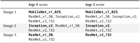
Table 1: List of models that give the correct prediction per image under the top-5 and the top-1 scores.

top-5score top-1score

Image 1 MobileNet_v1_025,

ResNet_v1_50,Inception_v2,

ResNet_v2_152

MobileNet_v1_025,

ResNet_v1_50,Inception_v2,

ResNet_v2_152

Image 2 Inception_v2,ResNet_v1_50,

ResNet_v2_152

Inception_v2,

ResNet_v2_152

Image 3 ResNet_v1_50,

ResNet_v2_152

ResNet_v2_152

output. Overall, it improves the inference accuracy by 7.52% over the most-capable, single model but with 1.8x less inference time.

This paper makes the following contributions:

• We present a novel machine learning based approach to automatically learn how to selectDNNmodels based on the input and precision requirement (Section 3); • Our work is the first to leverage multipleDNNmodels

to improve the prediction accuracy and reduce inference time on embedded systems (Section 5). Our automatic approach allows developers to easily re-target the approach for newDNNmodels and user requirements;

• Our system has little training overhead as it does not require any modification to pre-trainedDNNmodels.

2

MOTIVATION AND OVERVIEW

2.1

Motivation

As a motivating example, consider performing object recognition on a NVIDIA Jetson TX2 platform.

Setup.In this experiment, we compare the performance of

three influential Convolutional Neural Network (CNN) architectures: Inception [23], ResNet [18], and MobileNet [19]3_{. Specifically, we used the following}

3 _{Each model architecture follows its own naming convention.}

MobileNet_vi_j, where i is the version number, and j is a width multiplier out of 100, with 100 being the full uncompressed model.

ResNet_vi_j, whereiis the version number, andjis the number of layers

models: MobileNet_v1_025, the MobileNet architecture with a width multiplier of 0.25; ResNet_v1_50, the first version of ResNet with 50 layers; Inception_v2, the second version of Inception; and ResNet_v2_152, the second version ofResNetwith 152 layers. All these models are built upon TensorFlow [1] and have been pre-trained by independent researchers using the ImageNet ILSVRC 2012

training dataset[39]. We use the GPU for inference.

Evaluation Criteria.Each model takes an image as input

and returns a list of label confidence values as output. Each value indicates the confidence that a particular object is in the image. The resulting list of object values are sorted in descending order regarding their prediction confidence, so that the label with the highest confidence appears at the top of the list. In this example, the accuracy of a model is evaluated using thetop-1and thetop-5scores defined by the ImageNet Challenge. Specifically, for thetop-1score, we check if the top output label matches the ground truth label of the primary object; and for thetop-5score, we check if the ground truth label of the primary object is in the top 5 of the output labels for each given model.

Results.Figure 1d shows the inference time per model

using three images from the ImageNet ILSVRCvalidation dataset. Recognizing the main object (a cottontail rabbit) from the image shown in Figure 1a is a straightforward task. We can see from Figure 1 that all models give the correct answer under thetop-5andtop-1score criterion. For this image,MobileNet_v1_025is the best model to use under

thetop-5score, because it has the fastest inference time –

6.13x faster thanResNet_v2_152. Clearly, for this image, MobileNet_v1_025is good enough, and there is no need to use a more advanced (and more expensive model) for inference. If we consider a slightly more complex object recognition task shown in Figure 1b, we can see that MobileNet_v1_025 is unable to give a correct answer regardless of our success criterion. In this case Inception_v2should be used, although this is 3.24x slower thanMobileNet_v1_025. Finally, consider the final image shown in Figure 1c, intuitively it can be seen that this would be a more difficult image recognition task, this main object is a similar color to the background. In this case the model we should use changes depending on our success criterion. ResNet_v1_50is the best model to use under the top-5

score, completing inference 2.06x faster than ResNet_v2_152. However, if we instead use top-1 for scoring we must useResNet_v2_152to obtain the correct label, despite that it’s the most expensive model. Inference time for this image is 2.98x and 6.14x slower than MobileNet_v1_025 for top-5 and top-1 scoring respectively.

Feature

Extraction Inference

1 2 3 4

Offline Profiling Runs

Memory footprint Training

programs

Model Fitting

Feature Extraction

f Memory function

Feature values

5

Model Selection

Image Labels

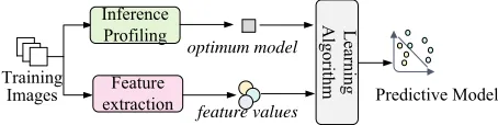
Figure 2: Overview of our approach

Y Model 1 Input

features

Distance

calculation Model 1? N

Model 2?

Model 2 N

Model n?

Model n N

KNN-1 KNN-2 KNN-n

all models will fail

...

Y Y

Figure 3: Our premodel, made up of a series of KNN

models. Each model predicts whether to use an image classifier or not, our selection process for including image classifiers is described in Section 3.2.

Lessons Learned.This example shows that the best model

depends on the input and the evaluation criterion. Hence, determining which model to use is non-trivial. What we need is a technique that can automatically choose the most efficient model to use for any given input. In the next section, we describe our adaptive approach that solves this task.

2.2

Overview of Our Approach

Figure 2 depicts the overall work flow of our approach. While our approach is generally applicable, to have a concrete, measurable target, we apply it to image classification. At the core of our approach is a predictive model (termedpremodel) that takes anew, unseenimage to predict which of a set of pre-trained image classification models to use for the given input. This decision may vary depending on the scoring method used at the time, e.g., eithertop-1ortop-5, and we show that our approach can adapt to different metrics.

The prediction of our premodel is based on a set of quantifiable properties – orfeaturessuch as the number of edges and brightness – of the input image. Once a model is chosen, the input image is passed to the selected model, which then attempts to classify the image. Finally, the classification data of the selected model is returned as outputs. Use of ourpremodelwill work in exactly the same way as any single model, the difference being we are able to choose the best model to use dynamically.

3

OUR APPROACH

Ourpremodelis made up of multiple k-Nearest Neighbour (KNN) classification models arranged in sequence, shown in Figure 34. As input our model takes an image, from which it will extract features and make a prediction, outputting a label referring to which image classification model to use.

4_{In Section 5.2, we evaluate a number of different machine learning}

LCTES ’18, June 2018, Pennsylvania, USA web

content

Parsing

Style Resolution

Layout

Paint

Display

DOM Tree

Style Rules

Render Tree

Training Images

Inference Profiling

Feature extraction

optimum model

feature values

Learning

A

lgorithm

Predictive Model Kernel on

CPU

Kernel on Accelerator

CPU config.

accelerator config.

host CPU config.

Figure 4: The training process. We use the same procedure to train each individual model within the

premodelfor each evaluation criterion.

3.1

Model Description

There are two main requirements to consider when developing an inferencing model selection strategy on a embedded device: (i) fast execution time, and (ii) a high level of accuracy. Having apremodelwhich takes much longer than any single model would outweigh the benefit of using it. We also require high accuracy to choose the optimum inferencing model, therefore reducing the oveall cost.

Following the above goals we chose to implement a series of simpleKNNmodels, where each model predicts whether to use a single image classifier or not. We choseKNNas it has a quick prediction time (less than 1ms) and achieves a high accuracy for our problem. Finally, we chose a set of features to represent each image, the selection process of these features is described in more detail in Section 3.4.

Figure 3 gives an overview of ourpremodelarchitecture. For eachDNNmodel we wish to include in ourpremodel, we use a separateKNNmodel. As ourKNNmodels are going to contain much of the same data we begin ourpremodelby calculating our K closest neighbours. Taking note of which record of training data each of the neighbours corresponds to, we are able to avoid recalculating the distance measurements; we simply change the labels of these data-points.KNN-1is the firstKNNmodel in ourpremodel, through which all input to thepremodelwill pass.KNN-1is used to predict whether the input image should useModel-1 to classify it or not, depending on the scoring criterion thepremodelhas been trained for. IfKNN-1predicts thatModel-1should be used, then thepremodelreturns this label, otherwise the features are passed on to the nextKNN,i.e. KNN-2. This process carries on until the image reachesKNN-n, the finalKNNmodel in our premodel. In the event thatKNN-npredicts that we should not useModel-nto classify the image, the next step will be one of two depending on the user’s declared preference: (i) using a pre-specified model, so the user can have some output to work with; or (ii) do not perform inference and simple informing the user of the failure.

3.2

Inference Model Selection

In Algorithm 1 we describe our selection process for choosing which inference models to include in our premodel. Essentially, this algorithm involves choosing the first model to include, which is always the one which is

Algorithm 1Inference Model Selection Process

Model_1_class=most_optimum_class(data) curr_class.add(Model_1_class)

curr_acc=дet_acc(curr_class)

acc_diff = 100 whileacc_diff>θdo

failed_cases = get_fail_cases(curr_class) next_class = most_acc_class(failed_cases)

curr_class.add(next_class) new_acc=дet_acc(curr_class)

acc_diff = new_acc - curr_acc

curr_acc=new_acc

end while

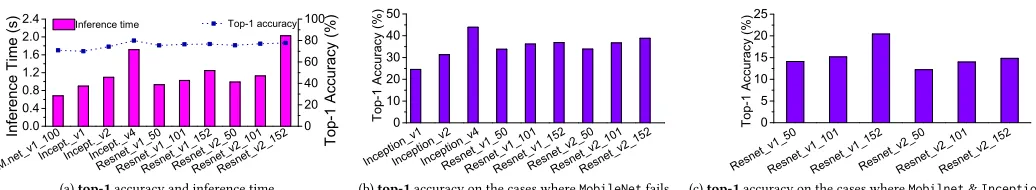
optimal for the most of our training data, then iteratively adding the most accurate model on the remainder of the training data until our accuracy improvement is lower than a thresholdθ. Below we will walk through the algorithm to show how we chose the model to include in ourpremodel. We have chosen to set our threshold value, θ to 0.5, which is empirically decided during our pilot experiments. Figure 5 shows the percentage of our training data which considers each of ourCNNsto be optimal. There is a clear winner here, MobileNet_v1_100is optimal for 70.75% of our training data, therefore it is chosen to beModel-1for our premodel. If we were to follow this convention and then choose the next most optimalCNN, we would choose Inception_v1. However, we do not do this as it would result in ourpremodelbeing formulated of many cheap, yet inaccurate models. Instead we choose to look at the training data on which our initial model (Model-1) fails; the remaining 29.25% of our data.

From here on when adding newCNNsto ourpremodel we exclusively consider the accuracy of each on the currently failing training data. Figure 6b shows the accuracy of our remaining CNNs on the 29.25% cases where MobileNet_v1_100fails. We can see that Inception_v4 clearly wins here, correctly classifying 43.91% of the remaining data; creating a 12.84% increase in premodel accuracy, and leaving 16.41% of our data failing. We then repeat this process, shown in Figure 6c, where we add ResNet_v1_152to ourpremodelseeing an increase in total accuracy of 2.55%. Finally we repeat this step one more time, to achieve apremodelaccuracy increase of <0.5, therefore <θ, and terminate here.

The result of this is a premodel where: Model-1 is MobileNet_v1_100,Model-2isInception_v4, and, finally,

Model-3isResNet_v1_152.

3.3

Training the

premodel

Table 2: All features considered in this work.

Feature Description Feature Description

n_keypoints # of keypoints avg_brightness Average brightness

brightness_rms Root mean square of brightness avg_perceived_brightness Average of perceived brightness

perceived_brightness_rms Root mean square of perceived brightness contrast The level of contrast

edge_length{1-7} A 7-bin histogram of edge lengths edge_angle{1-7} A 7-bin histogram of edge angles

area_by_perim Area / perimeter of the main object aspect_ratio The aspect ratio of the main object

hue{1-7} A 7-bin histogram of the different hues

M . ne t _ v 1 _ 10 0

I n c ep t i o n _ v1 R e sn e t _

v 1 _5 0 I n c ep t i o

n _ v2 R e sn e t _

v 2 _5 0 I n c ep t i o

n _ v3 R e sn e t _

v 1 _1 0 1 I n c ep t i o

n _ v4 R e sn e t _

v 2 _1 0 1 R e sn e t _

v 2 _1 5 2 R e sn e t _

v 1 _1 5 2

0

2 0 4 0 6 0 8 0

%

o

f b

ei

ng

o

pt

im

al

Figure 5: How often aCNNmodel is considered to be

optimal under the top-1 score on the training dataset.

process in detail below, and provide a summary in Figure 4. Generally, we need to figure out which candidate inferecing model is optimum for each of our training example (i.e., images), we then train our model to predict the same for anynew,unseeninputs.

Generate Training Data.Our training dataset consists of

the feature values of a set of images and the corresponding optimum model for each image under an evaluation criterion. To evaluate the performance of the candidateDNN models, they must be applied to unseen images. We choose to use ILVRSC 2012 validation set, which contains 50k images, to generate training data for ourpremodel. This dataset provides a wide selection of images containing a range of topics and complexities. We then exhaustively executed each image on each candidate model, measuring the inference time and prediction results. Inference time is measured on an unloaded machine to reduce noise, and is a one-off cost – it only needs to be completed once. Because the relative runtime of models is stable, training data generation can be performed on a high-performance server to speedup the training data generation process. It is to note that adding a new image classifier, simply requires executing all images on the new image classifier while taking the same measurements described above.

Taking the execution time,top-1, andtop-5results we are able to generate abestimage classifier for each image; that is, the model which achieves the accuracy goal (top-1

ortop-5) in the least amount of time. Finally, we extract the

feature values (described in Section 3.4) from each image, and pair the feature values to the best image classifier for each image, resulting in our complete training dataset.

Building the Model.The training data is used to determine

which classification models should be used and the optimal

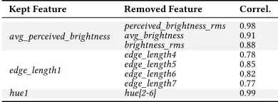
Table 3: Correlation values (absolute) of removed features to the kept ones.

Kept Feature Removed Feature Correl. perceived_brightness_rms 0.98

avg_brightness 0.91

avg_perceived_brightness

brightness_rms 0.88

edge_length4 0.78

edge_length5 0.85

edge_length6 0.82

edge_length1

edge_length7 0.77

hue1 hue{2-6} 0.99

hyper-parameters of the model. Since we chose to useKNN models to construct ourpremodel, the generated training data is used to train our model using a standard supervized learning method. InKNNclassification the training data is used to give a label to each point in the model, then during prediction the model will use a distance measure (in our case we use Euclidian distance) to find the K nearest points (in our case K=5). The label with the highest number of points to the prediction point is the output label.

Training Cost. Total training time of our premodel is

dominated by generating the training data. Generating the training data took less than a day using a NVIDIA P40 GPU on a multi-core server. This can vary depending on the number of image classifiers to be included. In our case, we had an usually long training time as we considered 12DNN models. We would expect in deployment that the user has a much smaller search space for image classifiers. The time in model selection and parameter tuning is negligible (less than 2 hours) in comparison. See also Section 5.5.

3.4

Features

One of the key aspects in building a successful predictor is developing the right features in order to characterize the input. In this work, we considered a total of 30 candidate features, shown in Table 2. The features were chosen based on previous image classification work [16] e.g., edge based features, as well as intuition based on our motivation (Section 2.1), e.g., contrast.

3.4.1 Feature selection.The time spent in making a

LCTES ’18, June 2018, Pennsylvania, USA

M . ne t _ v 1 _ 10 0

I n c ep t . _ v 1 I n c ep t . _

v 2 I n c ep t . _

v 4

R e sn e t _ v 1 _5 0 R e sn e t _

v 1 _1 0 1 R e sn e t _

v 1 _1 5 2 R e sn e t _

v 2 _5 0 R e sn e t _

v 2 _1 0 1 R e sn e t _

v 2 _1 5 2 0 . 0

0 . 4 0 . 8 1 . 2 1 . 6 2 . 0 2 . 4

In

fe

re

nc

e

Ti

m

e

(s

) _{I n f e r e n c e t i m e}

0

2 0 4 0 6 0 8 0 1 0 0

T o p - 1 a c c u r a c y

T

op

-1

A

cc

ur

ac

y

(%

)

I n c ep t i o n _ v1 I n c ep t i o

n _ v2 I n c ep t i o

n _ v4 R e sn e t _

v 1 _5 0 R e sn e t _

v 1 _1 0 1 R e sn e t _

v 1 _1 5 2 R e sn e t _

v 2 _5 0 R e sn e t _

v 2 _1 0 1 R e sn e t _

v 2 _1 5 2

0

1 0 2 0 3 0 4 0 5 0

To

p-1

Ac

cu

ra

cy

(%

)

R e sn e t _ v 1 _5 0 R e sn e t _

v 1 _1 0 1 R e sn e t _

v 1 _1 5 2 R e sn e t _

v 2 _5 0 R e sn e t _

v 2 _1 0 1 R e sn e t _

v 2 _1 5 2

0

5

1 0 1 5 2 0 2 5

To

p-1

Ac

cu

ra

cy

(%

)

(a)top-1accuracy and inference time (b)top-1accuracy on the cases whereMobileNetfails (c)top-1accuracy on the cases whereMobilnet&Inceptionfails

Figure 6: (a) Shows the top-1 accuracy and average inference time of allCNNsconsidered in this work across our

entire training dataset. (b) Shows the top-1 accuracy of allCNNson the images on whichMobileNet_v1_100fails.

(c) Shows the top-1 accuracy of allCNNson the images on whichMobileNet_v1_100andInception_v4fails.

Table 4: The chosen features.

n_keypoints avg_perceived_brightness hue1 contrast area_by_perim edge_length1 aspect_ratio

improving the generalization ability of ourpremodel, i.e.

reducing the likelihood of over-fitting on our training data. Initially, we use correlation-based feature selection. If pairwise correlation is high for any pair of features, we drop one of them and keep the other in order to retain most of the information. We performed this by constructing a matrix of correlation coefficients using Pearson product-moment correlation. The coefficient value falls between−1 and+1. The closer the absolute value is to 1, the stronger the correlation between the two features being tested. We set a threshold of 0.75 and removed any features that had an absolute Pearson correlation coefficient higher than the threshold. Table 3 summarizes the features we removed at this stage, leaving 17 features.

Next we evaluated the importance of each of our remaining features. To evaluate feature importance we first trained and evaluated our premodel using K-Fold cross validation (see also Section 5.5) and all of our current features, and recording premodel accuracy. We then remove each feature and re-evaluate the model on the remaining features, taking note of the change in accuracy. If there is a large drop in accuracy then the feature must be very important, otherwise, the features does not hold much importance for our purposes. Using this information we performed a greedy search, removing the least important features one by one. By performing this search we discovered that we can reduce our feature count down to 7 features (see Table 4) while having very little impact on our model accuracy. Removing any of the remaining 7 features resulted in a significant drop in model accuracy.

3.4.2 Feature scaling.The final step before passing our

features to a machine learning model is scaling each of the features to a common range (between 0 and 1) in order to prevent the range of any single feature being a factor in its importance. Scaling features does not affect the distribution

a s p e c t_ r a t i o n _ k e y p o i n t s_{a v g _ p e} r c . _ b r i gh t . c o n t r a ste d g e _ le n g t h 1

0

5

1 0 1 5 2 0

lo

st

a

cc

ur

ac

y

(%

)

Figure 7: The top five features which can lead to a high

loss in accuracy if they are not used in ourpremodel.

or variance of their values. To scale the features of a new image during deployment we record the minimum and maximum values of each feature in the training dataset, and use these to scale the corresponding features.

3.4.3 Feature analysis.Figure 7 shows the top 5

dominant features based on their impact on ourpremodel accuracy. We calculate feature importance by first training a premodelusing all 7 of our chosen features, and note the accuracy of our model. In turn, we then remove each of our features, retraining and evaluating ourpremodel on the other 6, noting the drop in accuracy. We then normalize the values to produce a percentage of importance for each of our features. It can be seen that each of our features hold a very similar level of importance, ranging between 18% and 11% for our most and least important feature respectively. The similarity of our feature importance is an indication that each of our features is able to represent distinct information about each image. all of which is important for the prediction task at hand.

3.5

Runtime Deployment

4

EXPERIMENTAL SETUP

4.1

Platform and Models

Hardware.We evaluate our approach on the NVIDIA Jetson

TX2 embedded deep learning platform. The system has a 64 bit dual-core Denver2 and a 64 bit quad-core ARM Cortex-A57 running at 2.0 Ghz, and a 256-core NVIDIA Pascal GPU running at 1.3 Ghz. The board has 8 GB of LPDDR4 RAM and 96 GB of storage (32 GB eMMC plus 64 GB SD card).

System Software.Our evaluation platform runs Ubuntu

Ubuntu 16.04.3 LTS with Linux kernel v4.4.15. We use Tensorflow v.1.0.1, cuDNN (v6.0) and CUDA (v8.0.64). Our premodel is implemented using the Python scikit-learn machine learning package. Our feature extractor is built upon OpenCV and SimpleCV.

Deep Learning Models.We consider 14 pre-trainedCNN

models for image recognition from the TensorFlow-Slim library [40]. The models are built upon TensorFlow and trained on the ImageNet ILSVRC 2012 training set.

4.2

Evaluation Methodology

Model Evaluation. We use 10-fold cross-validation to

evaluate our premodel on the ImageNet ILSVRC 2012 validation set. Specifically, we partition the 50K validation images into 10 equal sets, each containing 5K images. We retain one set for testing ourpremodel, and the remaining 9 sets are used as training data. We repeat this process 10 times (folds), with each of the 10 sets used exactly once as the testing data. This standard methodology evaluates the generalization ability of a machine-learning model.

We evaluate our approach using the following metrics: • Inference time (lower is better). Wall clock time

between a model taking in an input and producing an output, including the overhead of ourpremodel. • Energy consumption (lower is better). The energy

used by a model for inference. For our approach, this also includes the energy consumption of the premodel. We deduct the static power used by the hardware when the system is idle.

• Accuracy (higher is better). The ratio of correctly labeled images to the total number of testing images. • Precision(higher is better). The ratio of a correctly predicted images to the total number of images that are predicted to have a specific object. This metric answers e.g., “Of all the images that are labeled to have a cat, how many actually have a cat?".

• Recall (higher is better). The ratio of correctly predicted images to the total number of test images that belong to an object class. This metric answers e.g., “Of all the test images that have a cat, how many are actually labeled to have a cat?".

• F1 score(higher is better). The weighted average of Precision and Recall, calculated as 2×Recal l_{Recal l}×₊P r ecision_{P r ecision}. It is useful when the test datasets have an uneven distribution of object classes.

Performance Report.We report the geometric meanof

the aforementioned evaluation metrics across the cross-validation folds. To collect inference time and energy consumption, we run each model on each input repeatedly until the 95% confidence bound per model per input is smaller than 5%. In the experiments, we exclude the loading time of theCNNmodels as the model only need to be loaded once in practice. However, we include the overhead of our premodelin all our experimental data. To measure energy consumption, we developed a lightweight runtime to take readings from the on-board energy sensors at a frequency of 1,000 samples per second. We then matched the energy readings against the time stamps of model execution to calculate the energy consumption.

5

EXPERIMENTAL RESULTS

5.1

Overall Performance

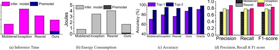
Inference Time.Figure 8a compares the inference time

among individualDNNmodels and our approach.MobileNet is the fastest model for inferencing, being 2.8x and 2x faster than Inception and ResNet, respectively, but is least accurate (see Figure 8c). Ourpremodelalone is 3x faster thanMobileNet. Most the overhead of ourpremodelcomes from feature extraction. The average inference time of our approach is under a second, which is slightly longer than the 0.7 second average time ofMobileNet. Our approach is 1.8x faster thanInception, the most accurate inference model in our model set. Given that our approach can significantly improve the prediction accuracy ofMobilenet, we believe the modest cost of ourpremodelis acceptable.

Energy Consumption. Figure 8b gives the energy

LCTES ’18, June 2018, Pennsylvania, USA

M o b i l e n e t I n c e p t i o n R e s n e t O u r s

0

1

2

In

fe

re

nc

e

Ti

m

e

(s

) i n f e r . m o d e l P r e m o d e l

M o b i l e n e t I n c e p t i o n R e s n e t O u r s

0

1

2

3

4

5 I n f e r . m o d e l P r e m o d e l

Jo

ul

es

M o b i l e n e t I n c e p t i o n R e s n e t O u r s O r a c l e

4 0 6 0 8 0 1 0 0

Ac

cu

ra

cy

(%

) T o p - 1 T o p - 2

P r e c i s i o n R e c a l l F 1 - s c o r e 0 . 0

0 . 2 0 . 4 0 . 6 0 . 8

1 . 0 M o b i l e n e t I n c e p t i o n R e s n e t O u r s

(a) Inference Time (b) Energy Consumption (c) Accuracy (d) Precision, Recall & F1 score

Figure 8: Overall performance of our approach against individual models for inference time (a), energy consumption (b), accuracy (c), precision, recall and F1 score (d). Our approach gives the best overall performance.

C N N K N N D e c i s i o n T r e e s S V M

0 . 0 0 . 2 0 . 4 0 . 6 0 . 8

R

un

tim

e

(s

) R u n t i m e

0

2 0 4 0 6 0 8 0 1 0 0

T

op

-1

A

cc

ur

ac

y

(%

)

T o p - 1 A c c u r a c y

Figure 9: Comparison of alternative predictive

modeling techniques for building thepremodel.

Accuracy. Figures 8c compares the top-1 and top-5

accuracy achieved by each approach. We also show the best possible accuracy given by atheoreticallyperfect predictor for model selection, for which we callOracle. Note that the Oracledoes not give a 100% accuracy because there are cases where all the DNN models fail. By effectively leveraging multiple models, our approach outperforms all individual inference models. It improves the accuracy of MobileNetby 16.6% and 6% respectively for thetop-1and

thetop-5 scores. It also improves thetop-1 accuracy of

ResNet and Inception by 10.7% and 7.6% respectively. While we observe little improvement for thetop-5 score overInception– just 0.34% – our approach is 2x faster than it. Our approach delivers over 96% of the Oracle performance (87.4% vs 91.2% fortop-1and 95.4% vs 98.3%). Moreover, our approach never picks a model that fails while others can success. This result shows that our approach can improve the inference accuracy of individual models.

Precision, Recall, F1 Score.Finally, Figure 8d shows our

approach outperforms individual DNN models in other evaluation metrics. Specifically, our approach gives the highest overall precision, which in turns leads to the best F1 score. High precision can reduce false positive, which is important for certain domains like video surveillance because it can reduce the human involvement for inspecting false positive predictions.

5.2

Alternative Techniques for Premodel

Figure 9 shows thetop-1accuracy and runtime for using different techniques to construct thepremodel. Here, the learning task is to predict which of the inference models, MobileNet,Inception, andResNet, to use. In addition to KNN, we also considerCNNs, Decision Trees (DT) and Support

Vector Machines (SVM). We use the MobileNet structure, which is designed for embedded inference, to build the CNN-based premodel. We train all the models using the same training examples. We also use the same feature set for the KNN, DT, and SVM. For the CNN, we use a hyperparamter tuner [26] to optimize the training parameters, and we train the model for over 500 epochs.

While we hypothesized aCNNmodel to be effectively in predicting from an image to the output, the results are disappointing given its high runtime overhead. We suspect the low accuracy of the CNN is because the size of our cross-validation training set (that contains 45K images) is not sufficient for learning an effectiveCNN. Our chosenKNN model has a overhead that is comparable to theDTand the SVM, but has a higher accuracy. It is possible that the best technique can change as the application domain and training data size changes, but our generic approach for feature selection and model selection remains applicable.

Figure 10 shows the runtime andtop-1accuracy by using theKNN,DTandSVMto construct a hierarchicalpremodel of three levels. A configuration is denoted asX.Y.Z, where

X,Y andZ indicates the modeling technique for the first, second and third level of thepremodel, respectively. The result shows that our chosenpremodelorganization, (i.e., KNN.KNN.KNN), has the highesttop-1accuracy (87.4%) and the fastest running time (0.20 second). One of the benefits of using aKNNmodel in all levels is that the neighboring measurement only needs to be performed once as the results can be shared among models in different levels. This means the runtime overhead is nearly constant if we use theKNN across all hierarchical levels.

5.3

Impact of Inference Model Sizes

kn n. kn n. kn n kn n. kn n. dt kn n. kn n. sv m kn n. dt .k nn kn n. dt .d t kn n. dt .s vm kn n. sv m .k nn kn n. sv m .d t kn n. sv m .s vm dt .k nn .k nn dt .k nn .d t dt .k nn .s vm dt .d t.k nn dt .d t.d t dt .d t.s vm dt .s vm .k nn dt .s vm .d t dt .s vm .s vm sv m .k nn .k nn sv m .k nn .d t sv m .k nn .s vm sv m .d t.k nn sv m .d t.d t sv m .d t.s vm sv m .s vm .k nn sv m .s vm .d t sv m .s vm .s vm

0 . 0 0 . 2 0 . 4 0 . 6

Ru

nt

im

e

(s

) R u n t i m e

0

2 0 4 0 6 0 8 0 1 0 0

To p-1 Ac cu ra cy (% )

T o p - 1 A c c u r a c y

Figure 10: Using different modeling techniques to

form a 3-levelpremodel.

1 2 3 4 5

0 . 0 0 . 4 0 . 8 1 . 2 1 . 6 2 . 0 2 . 4

In fe re nc e Ti m e (s )

# I n f e r e n c e M o d e l s

I n f e r e n c e t i m e

0

2 0 4 0 6 0 8 0 1 0 0

T o p - 1 a c c u r a c y

T op -1 A cc ur ac y (% )

Figure 11: Overhead and achieved performance when

using different numbers ofDNNmodels for inferencing.

The min-max bars show the range of inference time across testing images.

n _ k ey p o ia s p en t sc t _ r a t i o

c o n tr a s t h u e 1 a r e a_ b y _

p e r i m

a v g _p e r c e i v ed _ b r

i g h t ne s s e d g e_ l e n

g t h 1 h u e 7 e d g e_ a n g

l e 5 e d g e_ l e n

g t h 3 e d g e_ a n g

l e 3 e d g e_ a n g

l e 6 e d g e_ a n g

l e 4 e d g e_ a n g

l e 7 e d g e_ a n g

l e 1 e d g e_ l e n

g t h 2 e d g e_ a n g

l e 2

0 6 1 2 1 8 lo st a cc ur ac y (% )

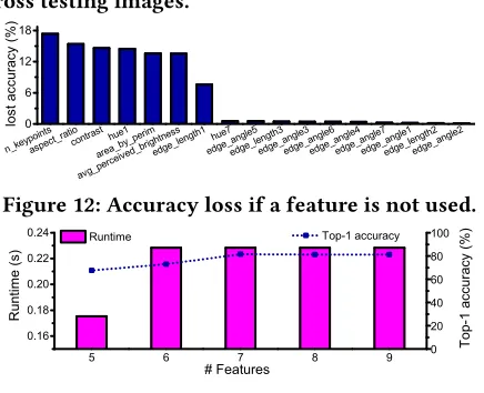
Figure 12: Accuracy loss if a feature is not used.

5 6 7 8 9

0 . 1 6 0 . 1 8 0 . 2 0 0 . 2 2 0 . 2 4

To p-1 ac cu ra cy (% ) R un tim e (s )

# F e a t u r e s

R u n t i m e

0

2 0 4 0 6 0 8 0 1 0 0 T o p - 1 a c c u r a c y

Figure 13: Impact of feature sizes.

likely to be chosen. At the same time, however, thetop-1

accuracy reaches a plateau of (≈87.5%) by using threeKNN models. We conclude that choosing threeKNNmodels would be the optimal solution for our case, as we are no longer gaining accuracy to justify the increased cost. This is in line with our choice of a value of 0.5 forθ.

5.4

Feature Importance

In Section 3.4 we describe our feature selection process, which resulted in using 7 features to represent each image to ourpremodel. In Figure 12 we show the importance of all of our considered features which were not removed by our correllation check, shown in Table 3. Upon observation it is clear that the 7 features we have chosen to keep are the most important; there is a sudden drop in feature

importance at feature 8 (hue7). Furthermore, in Figure 13 we show the impact onpremodelexecution time andtop-1

accuracy when we change the number of features we use. By decreasing the number of features there is a dramatic decrease top-1 accuracy, with very little change in extraction time. To reduce overhead, we would need to reduce our feature count to 5, however this comes at the cost of a 13.9% decrease intop-1accuracy. By increasing the feature count it can be seen that there is minor changes in overhead, but, surprisingly, there is actually also a small decrease in top-1 accuracy of 0.4%. From this we can conclude that using 7 features is ideal.

5.5

Training and Deployment Overhead

Training thepremodelis aone-off cost, and is dominated by the generation of training data which takes in total less than a day (see Section 3.3). This overhead can be speeded up using multiple machines. However, compared to the training time of a typicalDNNmodel, our training overhead is negligible.

The runtime overhead of our premodelis minimal, as depicted in Figures 8a. Out of a total average execution time of less than a second to classify an image, our premodel accounts for only 20%. In comparison to the most (ResNet_v2_152) and least (MobileNet) expensive models we consider in this work, this translates to 9.52% and 27%, respectively. Furthermore, our energy footprint is much smaller, making up 11% of the total cost. Comparing this to the most and least expensive models, again, gives an overhead of 7% and 25%, respectively.

6

DISCUSSION

Naturally there is room for further work and possible improvements. We discuss a few points here.

Alternative Domains.This work focuses onCNNsbecause

it is a commonly used deep learning architecture. To extend our work to other domains and recurrent neural networks (RNN), we would need a new set of features to characterize the input, e.g., text embeddings for machine translation [48]. However, our automatic approach on feature selection and premodelconstruction remains applicable.

Feature Extraction. The majority of our overhead is

caused by feature extraction for our premodel. Our prototype feature extractor is written in Python; by re-writing this tool in a more efficient language can reduce the overhead. There are also hotshots in our code which would benefit from parallelism.

Processor Choice. By default, inference is carried out on

LCTES ’18, June 2018, Pennsylvania, USA

Model Size.Our approach uses multiple pre-trainedDNN

models for inference. In comparison to the default method of simply using a single model, our approach would require more storage space. A solution for this would involve using model compression techniques to generate multiple compressed models from a single accurate model. Each compressed model would be smaller and is specialized at certain tasks. The result of this is numerous models share many weights in common, which allows us to allowing us to amortize the cost of using multiple models.

7

RELATED WORK

Deep neural networks (DNN) have shown astounding successes in various complex tasks that previously seemed difficult [7, 27, 30]. Despite the fact that many embedded devices require precise sensing capabilities, adoption ofDNN models on such systems has notably slow progress. The main cause of this slow progress is thatDNN-based inference is typically a computation intensive task, which inherently runs slowly on embedded devices due to limited resources.

Numerous methods have been proposed to reduce the computational demands of a deep model by trading prediction accuracy for runtime, via compressing a pre-trained network [6, 15, 21, 24, 36, 42, 47], training small networks directly [11, 37], or a combination of both [19]. Using these approaches, a user now needs to decide when to use a specific model, in order to meet the prediction accuracy requirement with minimal latency. This is because different models have different characteristics in terms of prediction accuracy and running time. It is a non-trivial task to make such a crucial decision as the application context (e.g. the model input) is often unpredictable and constantly evolving. Our work alleviates the user burden by automatically selecting the most appropriate model to use based on the application constraint and input context.

Neurosurgeon [25] identifies when it is beneficial to offload aDNN layer to be computed on the cloud. Unlike Neurosurgeon, we aim to minimize theon-deviceinference time without compromising prediction accuracy. Our work is useful in scenarios when sending data to the cloud is prohibitive due to e.g. poor network connectivity or privacy concerns. The Pervasive CNN framework [41] generates multiple computation kernels for each layer of aCNN, which are then dynamically selected according to the inputs and user constraints. A similar approach [38] trains a model twice, once on shared data and again on personal data, in an attempt to prevent personal data being sent outside the personal domain. In contrast to the latter two works, our approach allows having a diverse set of networks, by choosing the most effective network to use at runtime. They, however, are complementary to our approach, by providing the capability to fine-tune a single network structure.

Recently, numerous software-based approaches have been proposed to accelerate CNN models on embeded devices. They aim to accelerate inference time by exploiting parameter tuning [29], computational kernel optimization [3, 14], task parallelism [32] and partition [28, 35], and trading precision for time [20] etc. Since a single model is unlikely to meet all the constraints of accuracy, inference time and energy consumption across inputs [5, 13], it is attractive to have a strategy to dynamically select the appropriate model to use. Our work provides such a capability and is thus complementary to existing approaches onDNNmodel acceleration.

Off-loading computation to the cloud can accelerateDNN model inference [46], but this is not always applicable due to privacy, latency or connectivity issues. The work presented by Ossia et al. partially addresses the issue of privacy-preserving when offloading DNNinference to the cloud [33]. Our adaptive model selection approach allows one to select which model to use based on the input, and is also useful when cloud offloading is prohibitively because of the latency requirement or the lack of connectivity.

Predictive modeling has been employed in prior works to perform various optimization tasks, including application scheduling [12], approximate computing [22], code optimization [43] and hardware-software co-design [4]. No work so far has applied this technique to dynamically select deep learning models to run on embedded devices. Our approach is also closely related to ensemble learning where multiple models are used to solve an optimization problem. This technique is shown to be useful on scheduling parallel tasks [9] and optimize application memory usage [31]. This work is the first attempt in applying this technique to optimize deep inference on embedded devices.

8

CONCLUSION

REFERENCES

[1] JJ Allaire, Dirk Eddelbuettel, Nick Golding, and Yuan Tang. 2016.

TensorFlow for R. https://tensorflow.rstudio.com/

[2] Dzmitry Bahdanau, Kyunghyun Cho, and Yoshua Bengio. 2014. Neural

machine translation by jointly learning to align and translate.arXiv

preprint arXiv:1409.0473(2014).

[3] Sourav Bhattacharya and Nicholas D Lane. 2016. Sparsification and separation of deep learning layers for constrained resource inference

on wearables. InConference on Embedded Networked Sensor Systems.

ACM, 176–189.

[4] Bruno Bodin et al. 2016. Integrating Algorithmic Parameters

into Benchmarking and Design Space Exploration in 3D Scene

Understanding. InPACT.

[5] Alfredo Canziani, Adam Paszke, and Eugenio Culurciello. 2016. An Analysis of Deep Neural Network Models for Practical Applications.

CoRRabs/1605.07678 (2016).

[6] Wenlin Chen, James T. Wilson, Stephen Tyree, Kilian Q. Weinberger, and Yixin Chen. 2015. Compressing Neural Networks with the Hashing

Trick. InICML.

[7] Kyunghyun Cho, Bart van Merrienboer, Çaglar Gülçehre, Fethi Bougares, Holger Schwenk, and Yoshua Bengio. 2014. Learning phrase representations using RNN encoder-decoder for statistical machine

translation. InEMNLP.

[8] Jeff Donahue, Yangqing Jia, Oriol Vinyals, Judy Hoffman, Ning

Zhang, Eric Tzeng, and Trevor Darrell. 2014. DeCAF: A Deep

Convolutional Activation Feature for Generic Visual Recognition. In

ICML (Proceedings of Machine Learning Research), Eric P. Xing and Tony Jebara (Eds.), Vol. 32. PMLR, 647–655.

[9] Murali Krishna Emani and Michael O’Boyle. 2015. Celebrating

Diversity: A Mixture of Experts Approach for Runtime Mapping in

Dynamic Environments. InACM SIGPLAN Conference on Programming

Language Design and Implementation (PLDI ’15). 499–508.

[10] Dario Amodei et al. 2016. Deep Speech 2: End-to-End Speech

Recognition in English and Mandarin. InICML (Proceedings of Machine

Learning Research), Maria Florina Balcan and Kilian Q. Weinberger (Eds.), Vol. 48. PMLR, New York, New York, USA, 173–182.

[11] Petko Georgiev, Sourav Bhattacharya, Nicholas D. Lane, and Cecilia Mascolo. 2017. Low-resource Multi-task Audio Sensing for Mobile and Embedded Devices via Shared Deep Neural Network Representations.

Proc. ACM Interact. Mob. Wearable Ubiquitous Technol.1, 3 (2017), 50:1– 50:19.

[12] Dominik Grewe et al. 2013. Portable mapping of data parallel programs

to OpenCL for heterogeneous systems. InCGO.

[13] Tian Guo. 2017. Towards Efficient Deep Inference for Mobile

Applications.CoRRabs/1707.04610 (2017).

[14] Song Han, Xingyu Liu, Huizi Mao, Jing Pu, Ardavan Pedram, Mark A Horowitz, and William J Dally. 2016. EIE: efficient inference engine

on compressed deep neural network. In43rd International Symposium

on Computer Architecture. IEEE Press, 243–254.

[15] Song Han, Jeff Pool, John Tran, and William Dally. 2015. Learning both

weights and connections for efficient neural network. InAdvances in

neural information processing systems. 1135–1143.

[16] M Hassaballah, Aly Amin Abdelmgeid, and Hammam A Alshazly. 2016.

Image features detection, description and matching. InImage Feature

Detectors and Descriptors. 11–45.

[17] Kaiming He, Xiangyu Zhang, Shaoqing Ren, and Jian Sun. 2016. Deep

residual learning for image recognition. InConference on computer

vision and pattern recognition (CVPR). 770–778.

[18] Kaiming He, Xiangyu Zhang, Shaoqing Ren, and Jian Sun. 2016.

Identity mappings in deep residual networks. InEuropean Conference

on Computer Vision. Springer, 630–645.

[19] Andrew G. Howard, Menglong Zhu, Bo Chen, Dmitry Kalenichenko, Weijun Wang, Tobias Weyand, Marco Andreetto, and Hartwig Adam. 2017. Mobilenets: Efficient convolutional neural networks for mobile

vision applications.arXiv preprint arXiv:1704.04861(2017).

[20] Loc N. Huynh, Youngki Lee, and Rajesh Krishna Balan. 2017. DeepMon: Mobile GPU-based Deep Learning Framework for Continuous Vision

Applications. InMobiSys. 82–95.

[21] Forrest N. Iandola, Matthew W. Moskewicz, Khalid Ashraf, Song Han, William J. Dally, and Kurt Keutzer. 2016. SqueezeNet: AlexNet-level

accuracy with 50x fewer parameters and <1MB model size. CoRR

abs/1602.07360 (2016).

[22] Mohsen Imani, Yeseong Kim, Abbas Rahimi, and Tajana Rosing. 2016. ACAM: Approximate Computing Based on Adaptive Associative

Memory with Online Learning. InISLPED.

[23] Sergey Ioffe and Christian Szegedy. 2015. Batch normalization:

Accelerating deep network training by reducing internal covariate

shift. InICML.

[24] Jonghoon Jin, Aysegul Dundar, and Eugenio Culurciello. 2015.

Flattened Convolutional Neural Networks for Feedforward

Acceleration. (2015).

[25] Yiping Kang, Johann Hauswald, Cao Gao, Austin Rovinski, Trevor

Mudge, Jason Mars, and Lingjia Tang. 2017. Neurosurgeon:

Collaborative Intelligence Between the Cloud and Mobile Edge. In

ASPLOS.

[26] Aaron Klein, Stefan Falkner, Simon Bartels, Philipp Hennig, and Frank Hutter. 2016. Fast bayesian optimization of machine learning

hyperparameters on large datasets. arXiv preprint arXiv:1605.07079

(2016).

[27] Alex Krizhevsky, Ilya Sutskever, and Geoffrey E. Hinton. 2012. ImageNet classification with deep convolutional neural networks. In

NIPS.

[28] Nicholas D Lane, Sourav Bhattacharya, Petko Georgiev, Claudio Forlivesi, Lei Jiao, Lorena Qendro, and Fahim Kawsar. 2016. DeepX: A software accelerator for low-power deep learning inference on mobile

devices. InConference on Information Processing in Sensor Networks

(IPSN). IEEE, 1–12.

[29] Seyyed Salar Latifi Oskouei, Hossein Golestani, Matin Hashemi, and Soheil Ghiasi. 2016. Cnndroid: GPU-accelerated execution of

trained deep convolutional neural networks on android. InMultimedia

Conference. ACM, 1201–1205.

[30] Honglak Lee, Peter Pham, Yan Largman, and Andrew Y. Ng. 2009. Unsupervised Feature Learning for Audio Classification Using

Convolutional Deep Belief Networks. InNIPS.

[31] Vicent Sanz Marco, Ben Taylor, Barry Porter, and Zheng Wang. 2017. Improving Spark Application Throughput via Memory Aware Task

Co-location: A Mixture of Experts Approach. InMiddleware Conference.

95–108.

[32] Mohammad Motamedi, Daniel Fong, and Soheil Ghiasi. 2017. Machine Intelligence on Resource-Constrained IoT Devices: The Case of Thread

Granularity Optimization for CNN Inference. ACM Trans. Embed.

Comput. Syst.16 (2017), 151:1–151:19.

[33] Seyed Ali Ossia, Ali Shahin Shamsabadi, Ali Taheri, Hamid R Rabiee,

Nic Lane, and Hamed Haddadi. 2017. A Hybrid Deep Learning

Architecture for Privacy-Preserving Mobile Analytics.arXiv preprint

arXiv:1703.02952(2017).

[34] Omkar M Parkhi, Andrea Vedaldi, Andrew Zisserman, et al. 2015. Deep

Face Recognition. InBMVC, Vol. 1. 6.

[35] Sundari K. Rallapalli, H. Qiu, Archith John Bency, S. Karthikeyan, and

R. B. Govindan. 2016.Are Very Deep Neural Networks Feasible on Mobile

Devices?Technical Report 16-965. University of Southern California. [36] Mohammad Rastegari, Vicente Ordonez, Joseph Redmon, and Ali

LCTES ’18, June 2018, Pennsylvania, USA

Convolutional Neural Networks.CoRRabs/1603.05279 (2016).

[37] Sujith Ravi. 2015. ProjectionNet: Learning Efficient On-Device Deep

Networks Using Neural Projections.arXiv:1708.00630(2015).

[38] Sandra Servia Rodríguez, Liang Wang, Jianxin R. Zhao, Richard Mortier, and Hamed Haddadi. 2017. Personal Model Training under Privacy

Constraints.CoRRabs/1703.00380 (2017).

[39] Olga Russakovsky et al. 2015. ImageNet Large Scale Visual Recognition

Challenge. InIJCV.

[40] Nathan Silberman and Sergio Guadarrama. 2013.

TensorFlow-slim image classification library.

https://github.com/tensorflow/models/tree/master/research/slim. (2013).

[41] Mingcong Song, Yang Hu, Huixiang Chen, and Tao Li. 2017. Towards Pervasive and User Satisfactory CNN across GPU Microarchitectures.

InHPCA.

[42] Jost Tobias Springenberg, Alexey Dosovitskiy, Thomas Brox, and

Martin A. Riedmiller. 2014. Striving for Simplicity: The All

Convolutional Net.CoRRabs/1412.6806 (2014).

[43] Kevin Stock, Louis-Noël Pouchet, and P. Sadayappan. 2012. Using

machine learning to improve automatic vectorization. ACM

Transactions on Architecture and Code Optimization(2012).

[44] Yi Sun, Yuheng Chen, Xiaogang Wang, and Xiaoou Tang. 2014. Deep learning face representation by joint identification-verification. In

Advances in neural information processing systems. 1988–1996. [45] Ben Taylor, Vicent Sanz Marco, and Zheng Wang. 2017. Adaptive

Optimization for OpenCL Programs on Embedded Heterogeneous

Systems. In18th ACM SIGPLAN/SIGBED Conference on Languages,

Compilers, and Tools for Embedded Systems (LCTES 2017). 11–20. [46] Surat Teerapittayanon, Bradley McDanel, and HT Kung. 2017.

Distributed deep neural networks over the cloud, the edge and end

devices. InICDCS. 328–339.

[47] Min Wang, Baoyuan Liu, and Hassan Foroosh. 2016. Factorized

Convolutional Neural Networks.CoRRabs/1608.04337 (2016).