Optimal dynamic resource allocation to prevent defaults

Optimal Dynamic Resource Allocation to Prevent

Defaults

U Ayesta, M Erausquin, E Ferreira, P Jacko

To cite this version:

U Ayesta, M Erausquin, E Ferreira, P Jacko. Optimal Dynamic Resource Allocation to Prevent

Defaults. 2016.

<

hal-01300681

>

HAL Id: hal-01300681

https://hal.archives-ouvertes.fr/hal-01300681

Submitted on 11 Apr 2016

HAL

is a multi-disciplinary open access

archive for the deposit and dissemination of

sci-entific research documents, whether they are

pub-lished or not.

The documents may come from

teaching and research institutions in France or

abroad, or from public or private research centers.

Optimal Dynamic Resource Allocation to Prevent Defaults

U. Ayesta

_{, M. Erausquin}

_{, E. Ferreira}

_{, P. Jacko}

a

_{LAAS-CNRS, Univ. de Toulouse, CNRS, Toulouse, France}

_{Univ. de Toulouse, LAAS, Toulouse, France}

c

_{UPV/EHU, University of the Basque Country, Bilbao, Spain}

d

_{Lancaster University, Department of Management Science, Lancaster, LA1 4YX, UK}

Abstract

We consider a resource allocation problem, where a rational agent has to decide how to share a limited amount of resources among different companies that might be facing financial difficulties. The objective is to minimize the total long term cost incurred by the economy due to default events. Using the framework of multi-armed restless bandits and, assuming a two-state evolution of the default risk, the optimal dynamic resource sharing policy is determined. This policy assigns an index value to each company, which orders its priority to be funded. We obtain an analytical expression for this index, which generalizes the return-on-investment (ROI) index under the static setting, and we analyse the influence of the future events on the optimal dynamic policy. A discussion about the structure of the optimal dynamic policy is provided, as well as some extensions of the model.

Keywords: Markov Decision Processes, Multi-Armed Bandit Problem, Default Risk Management, Dynamic Resource Allocation Policies.

1

Introduction

There are many situations where a rational agent (e.g. a public institution) spends a certain amount of resources in order to obtain social rewards (i.e. to prevent social losses). How to manage those resources in an optimal way is a problem that has been widely analysed in the literature. For instance, [2] developed models where the control instruments are income tax rate, government deficit size or debt-money ratio. These instruments are used to maximize functions defined in terms of certain social criteria (e.g. growth rate). In recent years, and more intensely due to economical and financial situation, economic agents have been facing the resource allocation problem of minimizing the social cost incurred by the economy when a firm defaults. Many countries have been sharing public resources among companies which have been close to default, in order to avoid social costs (e.g. sudden increase in unemployment due to collective redundancies) derived from the default event. Although there is a lot of literature devoted to the problem of how to deal with bank failures (see e.g. [1] and references there), to the best of our knowledge, there is not much literature modelling how to solve the resource allocation optimization problem to prevent defaults in a dynamic manner.

MARB problems are a class of sequential resource allocation problems concerned with allocating resources among several alternative arms in a competitive manner. Depending on how the resources are allocated, the dynamics of the states of the arms might change. Moreover, the rewards earned by the decision maker depend on the state of the arms. And, therefore, the decision maker has to find an optimal policy taking into account both the influence of the actions chosen in the dynamics of the states, and the reward structure of each arm. There is a large recent literature where similar models have been shown to be useful in a variety of application fields (see, for instance, [14, 9, 6], and the references therein). In some cases, the solution of MARB problems is easy to implement and analyse. The optimal policy is given in terms of the (Whittle) index function, which assigns an index value to each arm. The larger the index value of an arm is, the higher is its priority when resources are allocated. Therefore, if this index function is obtained analytically, it also gives some insights about the structure of the optimal policy.

The structure of the MARB framework fits to several problems in economics, where rational agents must allocate resources. For instance, [17] approached the problem in which a single firm is facing a market with unknown demand. [18] analyzed the possibility of mispricing in a two-armed bandit problem when the frequency of change is small. If several firms were to experiment independently in the same market, they might offer different prices in the long run. Optimal experimentation may therefore lead to price dispersion in the long run, as shown formally in [13]. [4] used both the MAB and MARB to identify the best strategy for managing obsolescence in such instances wherein organizations have to deal with continuous technological evolution under uncertainty. Another situation appears when we must choose between various research projects. [19] analyses this problem where each arm represents a different research project with an associated random. In [16] a richer model of choice between R & D processes is considered. The MARB problem has also been used for defining a canonical model of experimentation in teams. In [3] and [11] a set of players choose independently between the different arms.

In this paper, we propose the use of MARB to analyse a decision problem in a default risk framework. That is, a rational agent (referred as the decision maker) must face the problem of selecting how to share funds among different companies that might be facing risk of default. Those companies are competing to obtain those resources, in order to improve their financial situation and avoid the default. The goal of the rational agent is to minimize the long run average costs incurred by the default events.

Although we focus on default events related with firms in financial difficulties, the formulation presented in this paper could be adapted for approaching other resource allocation problems, where the objective is to keep as many individuals as possible in the system. For instance, similar models have been used in problems where resources are shared among patients [12], or human resources to maintain machinery [7]. The rest of the paper is organized as follows: the model, and the related optimization problem, are stated in Section2. In Section3, the dynamic optimal policy, characterized by an index function, is provided. In Section 4, we discuss the role of the parameters of the problem in the index function. Proofs are included in the Appendix.

2

Problem and model description

We consider a set K ={1,· · ·, K} of companies asking for funding. We assume that, every time the decision of allocating the available resources is taken, the companies are divided in two groups: those which have a positive probability of defaulting before the next decision period, and those which do not. For simplicity, we say that the state of the companies that belong to the first group isBad, and the state of the companies that are in the second group is Good.

Let us denote byck the cost incurred to the economy if company k∈ Kdefaults. For any periodt≥0, we

consider that, if company kdefaults at timet, the value of the costs derived from the default att= 0 is given by βtck, with 0≤β <1. In other words,βtis a discount factor that measures the present value of the cost of default

events at timet. Therefore, ifβ <1, the later a company defaults, the smaller the cost derived from the default is, since this cost will be multiplied by a discount factor. Thus, the discount factor represents the importance of the future given by the decision maker, and the decision maker will select the best value ofβaccording to its planning horizon. Clearly,β might include information related with inflation and, possibly, other future effects.

If the decision is not to give resources to companykwhile being inBad state, then, this company will default with probability dk. However, if the decision is to fund it, then the default probability is decreased toµkdk, with

0< µk<1. Both dk andµkdk can be interpreted as “expected probabilities”.

to companyk, in order to decrease its default probability. The evolution of the state of each company is modelled with a Markov chain, where the transition probabilities depend on the action taken by the decision maker (see (1) and (2)).

The objective is to find a policy which prescribes how to share the resources in order to minimize the expected total discounted costs derived from the defaults of the companies, given an expected budget per period. There is a clear trade-off related to the described optimization problem, between funding companies in the bad state versus funding companies in the good state. By giving funding to companies in the bad state, the decision maker obtains a reward in the short term. On the other hand, by funding companies in the good state, the decision maker prevents those companies from moving to the bad state, keeping them alive as long as possible.

We represent this optimization problem using a discrete-time MDP formulation, which fits in the framework of the MARB problem [20,14]. Consider the time slotted in periods,t∈ T ={0,1,· · · }. At each time period, some of the companies in K are selected to receive funding from the decision maker, according to a budget constraint. We denote by A = {0,1} the action space for each company, where 0 represents not selecting a company for funding, whereas 1 means selecting it. Each company is characterized independently from other companies, by the tuple N,(Wa

k)a∈A,(R

a

k)a∈A,(P

a k)a∈A

, where:

• N ={G, B, D}represents the state space of the company. State Grepresents the Good state,B represents theBad state, andDrepresents the company is default.

• W_ka=W_k,na

n∈N, whereW

a

k,nrepresents the one period budget consumption of companyk, being in state

n, if actionais taken by the decision maker. In particular, we have, for anyn∈ N,

Wk,n1 =wk Wk,n0 = 0

In other words, the amount of resources given iswk if companykis selected and 0 otherwise.

• Ra k =

Ra

k,n

n∈N, where R

a

k,n represents the one period expected reward earned by the system due to

companykat staten∈ N if actionais decided in the beginning of the period. In particular, in our model we have

R1_k,G = 0 R0_k,G= 0, R1k,B = −µkdkck R0k,B=−dkck,

R1_k,D = 0 R0_k,D= 0.

• P_ka = pa_k,m,n

m,n∈N represents the one-period probability of company k of migrating from state m to

statenif actionais taken by the decision maker. The following transition matrices describe the transition probabilities under different actions:

P1k:=

  

G B D

G p1

k,G,G p

1

k,G,B 0

B p1_k,B,G p1_k,B,B µkdk

D 0 0 1

 

 (1)

P0_k:=   

G B D

G p0_k,G,G p0_k,G,B 0 B p0

k,B,G p

0

k,B,B dk

D 0 0 1

 

 (2)

Note thatD is an absorbing state.

The dynamics of companyk is then captured by the state process (Xk(t))t∈T, and the action process (ak(t))t∈T.

As a result of deciding actionak(t) in stateXk(t), the company consumes the allocated funding, provides a reward,

2.1

Optimization problem

Let ΠX,a be the set of randomized and non-anticipative policies that at the beginning of periodt decide an

ac-tion a(t) = (a1(t), ..., aK(t))∈ AK based only on the evolution of the state space, X(0), X(1),· · · , X(t), where

X(t) = (X1(t), ..., XK(t) and the history of the action process, a(0), a(1),· · ·, a(t−1). Let Eπτ denote the

ex-pectation over the state process X(·) and over the action process a(·), conditioned on the state-process history X(0), X(1), . . . , X(τ) and on policyπ.

We formulate now the optimization problem we want to solve. For any 0≤β ≤1, the goal is to find a policy π∈ΠX,a that maximizes the expected total discounted reward starting from the initial time period 0, subject to

the family of sample path allocation constraints, i.e.,

max

π∈ΠX,a

Eπ0

"

∞

t=0

X

k∈K

βtRak(t)

k,Xk(t)

#

(3)

s. t. Eπ0

"_∞ X

t=0

X

k∈K

βtWak(t)

k,Xk(t)

#

≤W (4)

Note thatW represents the total budget that the decision maker can spend on average. It seems natural to consider this quantity as the present value of the discounted budgets available at each period. For instance, if we assume that the budget at each period is given by a fixed value ˜W,W could be interpreted asW =P∞

t=0β

t_{W˜ =}

˜

W

1−β, for any 0≤β <1. Forβ= 1, (3) becomes a total cost minimization problem. In Section4.3.2we argue why

in this case any feasible policy is optimal.

3

Dynamic optimal policy

Following the method given in [20], this optimization problem described in (3)-(4) can be approached using Lagrangian multipliers, and decomposing it intoK single-company subproblems.

Notice that any joint policyπ∈ΠX,adefinesK single-company policies,_eπk∈ΠX,ak, which depend on the

joint state-space process and action process. We will therefore analyse the single-company subproblem

max e

πk∈ΠX,ak

Eeπk

0

"∞

X

t=0

βtRak(t)

k,Xk(t)−νW

ak(t)

k,Xk(t)

#

, (5)

being ν the Lagrangian multiplier.

Thus, the main idea of our approach is to identify a set of optimal policiesπ_ek∗for each companyk, and using them to construct a joint policy π_e∗, which will be optimal for the maximization problem (3)-(4). The optimal policy is obtained assigning an index value, νk,n, to each state n∈ N under the so-called indexability condition

[14].

The optimization problem described in (5) is a standard MDP problem for any value ofν. It is known that there exists an optimal policy in ΠX,ak, which is deterministic, Markovian, and independent of the initial state

(see, for instance, [15, Chapter 6]). In particular, this implies the existence of an optimal policy which depends on company k-s state-process Xk(·). Therefore, in order to find an optimal policy, it is enough to focus on policies

that are described in terms of a subset of states, S ⊆ N, which prescribes to allocate resources to company k whenever the company is in staten∈ S. Thus, an optimal policy can be obtained by solving

max

S⊆NE S 0

"∞

X

t=0

βtRak(t)

k,Xk(t)−νW

ak(t)

k,Xk(t)

#

, (6)

Let us define ∆k,G,G =p1k,G,G−p0k,G,G and ∆k,B,G=p1k,B,G−p0k,B,G. To derive our main results, we assume

the following:

∆k,B,G

∆k,G,G

≥1 or ∆k,G,G = 0. (7)

Remark 1. Condition (7) implies that both differences, ∆k,B,G and ∆k,G,G, have the same sign. Clearly, the

in state G. Moreover, a negative sign leads to a trivial situation, where not funding is always optimal. In general situations, where ∆k,B,G>0 and∆k,G,G>0, and∆k,G,G>0, condition (7) implies that the effect of funding is

greater in companies in the Bad state than in companies being in stateG, which seems to be a realistic assumption.

Letfk denote the total discounted probability of hitting stateB if starting from stateG and not funding

company kin stateG. It can easily be seen that

fk=

βp0_k,G,B 1−βp0

k,G,G

. (8)

Note thatfk is decreasing inp0k,G,G.

Next we define the index values for companyk

1.

νk,D := 0. (9)

2.

νk,G :=

µkckdk

wk

φk

1−φk

, (10)

where

φk =−β

p1

k,G,G−p

0

k,G,G

fk+

p1

k,G,B−p

0

k,G,B

1−βp1

k,B,Gfk+p1k,B,B

. (11)

3.

νk,B=

ckdk

wk

(1−µk−θk), (12)

where

θk=β

p1_k,B,G−p0_k,B,Gfk+

p1_k,B,B−p0_k,B,B 1−βp0

k,B,Gfk+p0k,B,B

. (13)

We describe now the main theoretical results of this paper. First, for each company k, we establish an ordering between the states with respect to the optimal policy.

Proposition 3.1. Assume (7).

1. Suppose thatν >0 holds. Then, if it is optimal for Problem (5) to fund companyk in stateG, it is optimal to fund it in stateB as well. Moreover, it is never optimal to fund companyk in stateD.

2. Suppose thatν ≤0. Then, it is optimal for Problem (5) to fund companykin any staten∈ N.

Proof. See Appendix A.

Remark 2. Proposition 3.1 establishes a natural order between the states. Since the optimal policy is a threshold-type solution, the states can be ordered following the priority given by the optimal policy. Throughout the rest of the paper, we refer to this order using the following notation: D < G < B. In view of this, we define by Sn:N ={m∈ N :m > n} the subset of N with statesbiggerthan a given state n.

Theorem 3.2 (Whittle’s indexability). Assume (7). The following holds for Problem (5)

1. If ν≤νk,n, then it is optimal to fund company kif it is in state n∈ N.

where νk,n are given in (9), (10) and (12).

Proof. See Appendix B.

Theorem 3.2 characterizes the optimal policy for the single-company problem. The optimal policy for the joint problem (3) is built, employing at any period t, the policy given by Theorem3.2 to all the companies in

K. Thus, if the Lagrangian multiplierν is known by the decision maker, the optimal policy for the joint problem becomes very simple to implement. At the beginning of any periodt, the decision maker has to proceed as follows:

1. First, observe the current state of each companyk.

2. Second, depending on the current state, compute the index value of each companyk.

3. Third, assign wk units of resources to each company k with index value higher than ν. Companies with

index value smaller or equal toν are not funded within this decision period.

As usual in threshold type solutions, the value of the threshold parameter ν can be computed numerically, using the duality theory (see [14]).

4

Discussion

Theorem 3.2 gives the optimal solution to Problem (3) in terms of the index values given in Equations (9), (10) and (12).

Although in practice the implementation of the optimal policy requires a parameter estimation procedure, the theoretical analysis of the structure of the indices gives some insights of how the optimal policy behaves. Since these indices establish a priority to each company, it is worth looking at the influence of the different parameters in the indices, to have an idea of the role that each one plays. First, it is important to point out that the index values are nonnegative. Due to the indexability property, as pointed out in Remark 2, it is known that for any company k∈ K, νk,D ≤νk,G ≤νk,B. Since νk,D = 0, we have that the index is greater than 0 in the other two

states.

4.1

Dependence of the index on

c

,

d

and

w

Since the index values are positive both for state B andG, it is straightforward to see in (10) and (12) that the indices are increasing in ck anddk, and decreasing inwk.

These properties coincide with what we could expect from the optimal policy. If we consider two companies being in the same state, and with equal parameters except for the costs derived from a default, then it makes sense to give priority to the company with the highest cost. Similarly, if there is a big difference between the amount of resources needed by two companies, but the rest of parameters are of the same order, then it seems also natural to give resources to the company that needs less resources, because the other resources can be saved for the future. Thus, properties that were expected to be followed by the optimal resource sharing policy hold in our priority index policy. Moreover, the expressions of the indices provide further information. For instance, the priority given to a company is not only increasing onck and decreasing onwk. The index shows that the priority

is proportional to the ratio between the two, ck/wk. Thus, the higher this ratio is, the more priority should be

given by the decision maker.

4.2

Dependence of the index on transition probabilities

We observe that if p1_k,B,G−p0_k,B,G ≥ 0 (a realistic assumption, as noted in Remark 1), then it is easy to show thatθk is decreasing inp0k,G,G, and thereforeνk,B is increasing inp0k,G,G. This means that a company with higher

Parameters c w d µ p1_G,G p1_G,B p1_B,G p1_B,B p0_G,G p0_G,B p0_B,G p0_B,B

Company 1 10000 1000 0.7 0.7857 0.6 0.4 0.25 0.2 0.5 0.5 0.1 0.2 Company 2 60000 1000 0.7 0.7857 0.6 0.4 0.25 0.2 0.5 0.5 0.1 0.2

Table 1: Parameters that represent companies 1 and 2.

4.3

Influence of the discount factor

The importance that the decision maker gives to the future plays a really important role in this resource allocation problem. Thus, analysing the influence of β on the indices, and therefore, on the optimal policy, gives useful information that can be used when making a decision.

4.3.1 The β= 0 case

Ifβ= 0, the decision maker is said to bemyopic. She only cares about the expected cost incurred by the economy at only one time slot, and forgets about minimizing possible future costs. Therefore, the optimal policy is given by that policy that minimizes the one-period expected cost. This is well captured by the indices given in (10) and (12).

Ifβ = 0, from (10), we have thatb = 0, and therefore, νk,G = 0. That is, for those companies that are in

stateG, the probability of moving to stateD in only one time slot is 0, and therefore, there is no reason to give them any resources. Thus, in this case companies in stateGhave the lowest priority.

On the other hand, from (12), we obtain thata= 0, and therefore, νk,B = ck_wd_kk(1−µk) = _wck_k(dk−µkdk).

Thus, among those companies with the same ratio ck

wk, those with the biggest difference dk −µkdk will have

absolute priority, wheredk−µkdk represents the difference between the probabilities of moving to stateD in one

step, not giving and giving resources to the company, respectively.

An interesting interpretation of the indexνk,B whenβ = 0 is its coincidence with thereturn-on-investment

(ROI) index, as explained in Section 4.4. Moreover, since the decision maker is myopic, no information about the rest of transition probabilities is used when assigning priority to the companies.

4.3.2 The β= 1 case

If β = 1, we are considering the total cost case, which in our case is always finite since all companies end up in finite time in the absorbing stateD. This means that the cost incurred by the economy when a company defaults is the same, no matter when this default event happens, and therefore, there is no reason to keep companies in the economy as much time as possible. Since state D is absorbing, it is almost surely known that all the companies will reach state D in a finite time, which means that the cost incurred by the economy due to default events is independent of the policy, and is given byPK

k=1ck. Thus, all the policies are optimal for the optimization problem

described in (3).

Settingβ= 1 in the expression for the indices as obtained in Section 3 we obtain thatνk,G=νk,B =νk,D= 0.

Thus, the indices are not able to establish an order based on priority, assigning the same priority to all the companies.

4.3.3 The 0< β <1 case

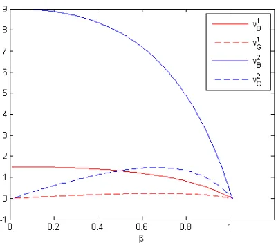
For 0< β <1, the indices depend on the transition probabilities. Not only the instantaneous transition probability to stateD matters, but also the evolution of the states in the future. An interesting property of the indices when 0 < β <1 is that, in some cases, it could be optimal to give resources to companies in stateG and, at the same time, not to give resources to some other companies in state B.

We illustrate this fact with the following numerical example. Consider two companies, described by the set of parameters given in Table1. The statistics that describe their evolution are the same, being the only difference that the cost incurred by the economy if Company 2 defaults is 6 times bigger than the cost when Company 1 defaults.

Figure 1: Comparison between indices

4.4

Comparison with ROI and Profitability Index

The return-on-investment (ROI) index is a fundamental and well-known performance measure often used in practice to evaluate investments and marketing expenditures. Broadly defined, ROI is the following measure:

ROI = Gain from investment - Cost of investment

Cost of investment . (14)

In particular the single-period ROI for our model is

ROIk,G+ 1 = 0, (15)

ROIk,B+ 1 =

ckdk

wk

(1−µk). (16)

It is interesting to note that the optimal myopic policy obtained from our proposed index in case β = 0 coincides with the single period ROI policy. Comparing ROIk,B+ 1 to the general index (12), we see that the

latter contains an extra term θk, which can be interpreted as anmulti-period adjustment.

Our index seems also related to theprofitability index (PI), which is defined as the following measure:

PI = Present value of future cashflows

Initial investment . (17)

It would be interesting to make an analogy and find out an interpretation for the terms in our proposed index.

Acknowledgements

The work of Urtzi Ayesta is partially supported by the French “Agence Nationale de la Recherche (ANR)” through the project ANR-15-CE25-0004 (ANR JCJC RACON). The work of Eva Ferreira, Martin Erausquin and Peter Jacko has been supported by MICINN (Ministerio de Ciencia e Innovaci´on), Spain, through grant MTM2010-17405 regarding Peter Jacko and grants ECO2011-29268 and ECO2014-51914-P regarding Eva Ferreira and Martin Erausquin.

References

[2] K.J Arrow and M. Kurz. Public Investment, The Rate of Return, and Optimal Fiscal Policy. Johns Hopkins University Press, 1970.

[3] P. Bolton and C. Harris. Strategic Experimentation. Econometrica, 67:349–374, 1999.

[4] U. Dinesh Kumar and H. Saranga. Optimal Selection of Obsolescence Mitigation Strategies Using a Restless Bandit Model. European Journal of Operational Research, 200:170–180, 2010.

[5] J.S. Fons. Using Default Rates to Model the Term Structure of Credit Risk. Financial Analysts Journal, pages 25–33, Sep./Oct. 1994.

[6] J.C. Gittins, K. Glazebrook, and R. Weber. Multi-armed Bandit Allocation Indices. Wiley, 2011.

[7] K. Glazebrook, Mitchell H., and P. Ansell. Index Policies for the Maintenance of a Collection of Machines by a Set of Repairment. European Journal of Operational Research, 165:267284, 2005.

[8] G.M. Gupton, C.C. Finger, and M. Bhatia. Credit metrics, technical document. Technical report, JP Morgan, 1997.

[9] P. Jacko. Dynamic Priority Allocation in Restless Bandit Models. Lambert Academic Publishing, 2010. Invited book.

[10] R.A Jarrow, D. Lando, and S.M Turnbull. A Markov Model for the Term Structure of Credit Risk Spreads. The Review of Financial Studies, 10(2):481–523, 1997.

[11] G. Keller, S. Rady, and M. Cripps. Strategic Experimentation with Exponential Bandits. Econometrica, 73:39–68, 2005.

[12] D. Li and K. Glazebrook. A Bayesian approach to the Triage Problem with Imperfect Classification.European Journal of Operational Research, 215:169180, 2011.

[13] A. McLennan. Price Dispersion and Incomplete Learning in the Long-Run. Journal of Economic Dynamics and Control, 7:331–347, 1984.

[14] J. Ni˜no-Mora. Dynamic priority allocation via restless bandit marginal productivity indices.TOP, 15(2):161– 198, 2007.

[15] M. L. Puterman. Markov Decision Processes: Discrete Stochastic Dynamic Programming. John Wiley & Sons, 2005.

[16] Weitzman Roberts. Funding Criteria for Research, Development and Exploration of Projects. Econometrica, 49:1261–1288, 1981.

[17] M. Rothschild. A Two-Armed Bandit Theory of Market Princing. Journal of Economic Theory, 9:185–202, 1974.

[18] A. Rustichini and A. Wolinsky. Learning About Variable Demand in the Long Run. Journal of Economic Dynamics and Control, 19:1283–1292, 1995.

[19] M.L. Weitzman. Optimal Seach for the Best Alternative. Econometrica, 47:641–654, 1979.

Appendix: Notation

Let us define the following quantities:

• ES0

h P∞

t=0β

t_Rak(t)

k,Xk(t)

i =_RS

n, being the initial stateXk(0) =n∈ N.

• ES0

h P∞

t=0β

t_Wak(t)

k,Xk(t)

i

=WSn, being the initial stateXk(0) =n∈ N.

The value function under policy S is given by

VSn =RSn−νWSn. (18)

Remark 3. Throughout the rest of the Appendices, we are solving a single-company subproblem that arises from the original optimization problem, say, for user k. Thus, in order to simplify the notation, we avoid writing the user subscript k.

Appendix A: Proof of Proposition

3.1

In Proposition3.1, we want to show that the optimal policy is of a threshold-type. Let us denote by_V∗

n the value

function following the optimal policy, under the staten∈ N. This value function satisfies the Bellman equation:

V∗n= max a∈A{R

a n−νW

a n+β

X

m∈N

pa_n,mV∗_n} (19)

For the three different states, using (19), we have that the optimal value function in given by

V∗B= max{ −µcd−νw+β q

1

B,GV

∗

G+q

1

B,BV

∗

B+µdV

∗

D

,

−cd+β qB,G0 V∗G+qB,B0 V∗B+dV∗D

} (20)

V∗G = max{ −νw+β q1G,GV∗G+q1G,BV∗B

,

β q0_G,GV∗_G+q0_G,BV∗_B

} (21)

V∗D= max{−νw+βV

∗

D, βV

∗

D}, (22)

where the first option in the brackets represents the value earned by the economy if the action 1 is taken in the current period, and the second option in the brackets represents action 0.

1. First, assume thatν >0. Sincew >0, it is clear that it is optimal not to fund this company, and we have V∗D= 0.From (18), it is easy to check that, for every policyπ∈Π, and for any initial staten∈ N,VSn ≤0.

Assume that it is optimal to fund a company in stateG. Then, by (21),

V∗G=−νw+β q

1

G,GV∗G+q

1

G,BV∗B

. (23)

Now, assume that it is not optimal to fund in stateB. Then, by (20)

V∗B =−cd+β q

0

B,GV∗G+q

0

B,BV∗B

. (24)

Our goal is to show that there is a contradiction in this case. (23) and (24) can be written as a system of two equations and two unknowns:

(

−βq_G,B1 _V∗_B+ 1−βq1_G,G

V∗G=−νw

1−βq0_B,BV∗B−βq

0

B,GV

∗

G=−cd

(25)

Using the first equation in (25), we can writeV∗B in terms ofV∗G as follows:

V∗B =

1−βq_G,G1 βq1

G,B

V∗G+

νw βq1

G,B

Since we are assuming that it is optimal to fund in stateG, from (21), we have that−νw+β q1

G,G−q0G,G

V∗G+ q1G,B−q0G,B

V∗B

> 0. Let us denote by ∆G,G=q1G,G−q0G,Gand ∆G,B=q1G,B−qG,B0 . Then, we have−νw+β(∆G,GV∗G+ ∆G,BV∗B)>

0. Sinceq1_G,B = 1−q1_G,G andq_G,B0 = 1−q0_G,G, ∆G,B=qG,B1 −q

0

G,B = 1−q

1

G,G−1 +q

0

G,G =−∆G,G, and

therefore, we obtain the following inequality:

−νw+β∆G,G(VG∗ −V∗B)>0. (27)

Using basic algebra, we obtain the simplified condition to be funded under stateG,

−∆G,G

q1

G,B

(νw+ (1−β)V∗G)> νw. (28)

Since we assume that it is not optimal to fund under stateB, from Equation (20),−µcd−νw+β q1

B,GV∗G+q

1

B,BV∗B

<

−cd+β q0

B,GV∗G+q0B,BV∗B

.Following the same steps as we did for state G, and using basic algebra, we obtain the following inequality:

νw+∆B,G

q1

G,B

(νw+ (1−β)V∗G) (29)

− d(1−µ)

c+_qνw1

G,B

−(1−βq 1 G,G) q1 G,B V ∗ G >0.

Our goal is to prove that, if (28) holds, then there must be a contradiction in (29). If ∆G,G = 0,

then this implication is true. If ∆G,G 6= 0, then introducing ∆G,G in previous expression, we obtain

νw+ ∆B,G

∆G,G

_∆

G,G

q1

G,B

(νw+ (1−β)_V∗_G)−d(1−µ)

c+ νw q1

G,B

−(1−βq 1 G,G) q1 G,B V ∗ G

> 0. However, it is easy to

show that there must be a contradiction in last inequality, since (28) holds, and using the fact that ∆G,G > 0 and ∆B,G > 0, V∗G ≤ 0 and

∆B,G

∆G,G > 1, we obtain νw+

∆B,G ∆G,G _∆ G,G q1 G,B

(νw+ (1−β)V∗G)

−

d(1−µ)

c+ νw q1

G,B

−(1−βq 1 G,G) q1 G,B V ∗ G

<0, which leads to the contradiction. Thus, assuming it is optimal to

fund a company under stateG, then it is optimal to fund this company under stateB as well.

2. If ν < 0, then, it is straightforward to see that the maximizing policy givesaπ_{(t) = 1 for all t, since the}

trade-off related to the optimization problem disappears. Funding at the period maximizes_RS_n, because the expected default time for the company is maximized. On the other hand, _WS_n is also maximized, since it addswat any period. Together withν <0, it is obvious to see that the value function is maximized as well.

Appendix B: Proof of Theorem

3.2

From definitions (4.4) and (4.4) we haveRSn =Rnn∈S +β

P

m∈Npnn,m∈SRSm andWSn =Wnn∈S+β

P

m∈Npnn,m∈SWSm.

To simplify the notation, the expression n∈ S is used in the superindex instead of the indicator functionIS(n).

That is,n∈ S equals 1 if true and 0 otherwise. Substituting the values ofRnn∈S,Wnn∈S andpnn,m∈S and simplifying,

we get the followingbalance equations:

Lemma 4.1.

RSG=

(

β p1_G,GRS_G+p1_G,BRS_B

if G∈ S,

β p0G,GRSG+p0G,BRSB

if G /∈ S, (30)

RSB=

(

−µcd+β p1B,GRSG+p1B,BRSB

ifB ∈ S,

−cd+β p0_B,GRGS +p0_B,BRS_B

ifB /∈ S, (31)

WSG=

(

w+β p1_G,GWS_G+p1_G,BWS_B

if G∈ S,

β p0_G,GWSG+p

0

G,BW

S

B

if G /∈ S, (32)

WSB=

(

w+β p1_B,GWSG+p

1

G,BW

S

B

if B∈ S, β p0_B,GWS_G+p0_B,BWS_B

Proof. Trivial from the definitions of_RS_n and_WS_n, for any n∈ N.

Following the methodology given in [14], we will studyνnunder all policiesS, defined asνnS := R

h1,Si n −R

h0,Si n

Whn1,Si−Whn0,Si

,

where byh1,Si(h0,Si) we refer to the policy that funds (does not fund) in the initial period and follows the strategy

S from that moment on.

Our objective is to find the optimal index valuesνn in terms of Theorem3.2. In other words, for each state

n∈ N, we have to find the action setS such that νn =νnS. This action set will be given by the following lemma

where we use the notationSn:N to refer to the subset ofN that are bigger thann.

Lemma 4.2. For alln∈ N,νn=νnSn:N, whereSn:N ={m∈ N :m > n}.

Proof. A sufficient condition to verify Lemma4.2is to show the LP-indexability, as described in [14], which in our problem can be simplified to the following:

Definition 1. Problem (5) is LP-indexable if the following conditions hold:

1. Wh1n,∅i−Wh0n,∅i≥0, andWnh1,N i−Wh0n,N i≥0, for alln∈ N.

2. Wh1n,Sn:Ni−Wnh0,Sn:Ni≥0, andWh1n+1,Sn:Ni−W h0,Sn:Ni

n+1 ≥0, for alln∈ N.

3. For every real-valuedν there existsn∈ N such that the policy defined by the set Sn:N is optimal.

It is easy to check that the conditions given in Definition 1 hold in our case. The first two conditions are straightforward and the third is already proved in Lemma4.2.

We use the action sets given in Lemma4.2to obtain the desired indices in terms of Theorem3.2. First, we calculate the index value of a company when its state isB. From Lemma4.2, we know thatνB =νBS, withS=∅.

This policy does not allocate any resources, no matter which the state of the company is, and we have that

ν_n∅:= R

h1,∅i

n −Rh0n,∅i

Wh1n,∅i−Wh0n,∅i

. (34)

First, it is clear that:

Rh1B,∅i−R

h0,∅i

B = (1−µ)cd+β

p1_B,G−p0_B,G

R∅G+ (p

1

B,B−p

0

B,B)R∅B

. (35)

On the other hand, we also have Wh1B,∅i−W

h0,∅i

B = w. The index value will be obtained solving the systems

obtained from the balance equations:

  

R∅B =−cd+β

p0_B,GR∅_G+p0_B,BR∅_B R∅G=β

p0_G,GR∅_G+p0_G,BR∅_B (36)

and we obtain that_Rh1_B,∅i−_RBh0,∅i= (1−µ)cd+β

(p1_B,G−p0_B,G)βp0_G,B

1−βp0

G,G

+ p1

B,B−p0B,B

R∅B.From (34), we obtain

the following index:

νB =

(1−µ)cd

w −

βcd

(p1_B,G−p0_B,G)βp0_G,B

1−βp0

G,G

+ p1

B,B−p0B,B

1−ββp

0

B,Gp0G,B

1−βp0

G,G

+p0

B,B

w

, (37)

that can be written asνB=cd(1−µ−θ)/w, where

θ= β

(p1

B,G−p0B,G)βp0G,B

1−βp0

G,G

+ p1_B,B−p0_B,B

1−ββp

0

B,Gp0G,B

1−βp0

G,G

+p0

B,B

Second, we calculate the index value when the company is in state G. In this case, from Lemma (4.2), it is clear that

νG=ν

{B}

G =

Rh1G,{B}i−R

h0,{B}i

G

Wh1G,{B}i−W

h0,{B}i

G

. (39)

First, we write (39) in terms ofRBB,R B G,W

B

B andW B

G. Following similar steps as in the first case, we obtain,

νG= R

h1,Bi

G −R

h0,Bi

G

Wh1G,Bi−W

h0,Bi

G

= µcd w

φ

1−φ, (40)

where

φ=−

β p1

G,G−p0G,G

βp0G,B

1−βp0

G,G

+ p1

G,B−p0G,B

1−ββp

1

B,Gp0G,B

1−βp0

G,G

+p1

B,B