Aerodynamics of gliding flight in common swifts

INTRODUCTION

From an aerodynamic viewpoint animal gliding flight is less complicated than flapping flight because it does not involve any moving actuators. A gliding animal should therefore comply more directly with aerodynamic theory, which has mainly been developed for fixed wing configurations. Yet, there are relatively few wind tunnel studies of gliding flight aerodynamics available (Pennycuick, 1968; Tucker and Parrott, 1970; Tucker and Heine, 1990; Rosén and Hedenström, 2001), probably because it requires a tiltable wind tunnel. Some basic properties about gliding flight can be measured in the field using an aircraft, an optical range finder or a radar (Pennycuick, 1971a; Pennycuick, 1971b; Tucker, 1988; Tucker et al., 1998; Rosén and Hedenström, 2002; Spaar and Bruderer, 1996; Spaar and Bruderer, 1997), but in such studies it is often not possible to record the body mass, wing morphology, horizontal and vertical winds.

The aerodynamic force generated by a flying bird is reflected in the vortex wake (e.g. Rayner, 1979a; Rayner, 1979b; Spedding, 1987), and modern techniques of digital particle image velocimetry (DPIV) have revealed both qualitative and quantitative properties about bird and bat wakes (e.g. Spedding et al., 2003; Hedenström et al., 2006; Hedenström et al., 2007; Rosén et al., 2007; Johansson et al., 2008; Hubel et al., 2009). However, only one study to date has investigated the wake shed from a gliding bird (Spedding et al., 1987), showing a rather simple wake consisting mainly of two wingtip vortices. In the present study, we used a tiltable wind tunnel (Pennycuick et al., 1997) and a stereo DPIV system to record the wake flow behind a common swift (Apus apusL.) in gliding flight. The advantage of this approach is that the sum of the aerodynamic forces lift (L) and drag (D) are known properties of a bird in steady

gliding flight, and we can use this for direct comparison with the contribution from the vortex wake.

The physics of gliding flight

A steadily gliding bird, i.e. non-powered flight with fixed wings at a constant flight speed, converts potential energy to counteract the aerodynamic forces. It will glide at a certain horizontal forward speed and sink speed. The sink speed (Us) will depend on the bird’s weight, wing morphology and body shape (streamlining). Sink speed is calculated as:

UsUsin, (1)

where Uis the flight speed along the glide path (not to be confused with horizontal speed) and is the angle of the glide path in relation to the horizontal (Fig.1). To standardize airspeed measurements, all speeds refer to equivalent airspeeds (UUtrue√/0), where Utrue is the true airspeed, is the average air density measured over each day of the experimental period and 01.225kgm–3is the standard air density at sea level). At equilibrium gliding, the resultant of lift and drag balances the weight of the bird (mass⫻gravity; mg). The lift component of the total force is directed perpendicular to the glide path. Note that lift in this case does not refer to the force keeping the bird aloft, but the force generated perpendicular to the wing surface (true lift). Lift is then given by:

Lmgcos. (2)

Drag of the bird is directed backwards, parallel to the glide path and perpendicular to lift and is calculated as:

Dmgsin. (3)

The Journal of Experimental Biology 214, 382-393 © 2011. Published by The Company of Biologists Ltd doi:10.1242/jeb.050609

RESEARCH ARTICLE

Aerodynamics of gliding flight in common swifts

P. Henningsson* and A. Hedenström

Department of Theoretical Ecology, Lund University, SE-223 62 Lund, Sweden

*Author for correspondence at present address: Animal Flight Group, Department of Zoology, University of Oxford, Oxford OX1 3PS, UK (per.henningsson@zoo.ox.ac.uk)

Accepted 28 September 2010

SUMMARY

Gliding flight performance and wake topology of a common swift (Apus apus L.) were examined in a wind tunnel at speeds between 7 and 11ms–1. The tunnel was tilted to simulate descending flight at different sink speeds. The swift varied its wingspan, wing area and tail span over the speed range. Wingspan decreased linearly with speed, whereas tail span decreased in a non-linear manner. For each airspeed, the minimum glide angle was found. The corresponding sink speeds showed a curvinon-linear relationship with airspeed, with a minimum sink speed at 8.1ms–1 _{and a speed of best glide at 9.4}_m_s–1_{. Lift-to-drag ratio was} calculated for each airspeed and tilt angle combinations and the maximum for each speed showed a curvilinear relationship with airspeed, with a maximum of 12.5 at an airspeed of 9.5ms–1_{. Wake was sampled in the transverse plane using stereo digital} particle image velocimetry (DPIV). The main structures of the wake were a pair of trailing wingtip vortices and a pair of trailing tail vortices. Circulation of these was measured and a model was constructed that showed good weight support. Parasite drag was estimated from the wake defect measured in the wake behind the body. Parasite drag coefficient ranged from 0.30 to 0.22 over the range of airspeeds. Induced drag was calculated and used to estimate profile drag coefficient, which was found to be in the same range as that previously measured on a Harris’ hawk.

Drag calculated in this manner represents the total drag of the bird. Drag of a flying bird is usually separated into three components: parasite drag, profile drag and induced drag. Parasite drag consists of friction and form drag of the body, caused when propelling the birds’ body through the air and is calculated as:

DparG SbCD,parU2, (4)

where is the air density, Sbis the body frontal area and CD,paris the parasite drag coefficient. Profile drag is the drag generated when moving the wings through the air and is calculated as:

DproG SwCD,proU2, (5) where Swis the wing area and CD,prois the profile drag coefficient. The third component is induced drag and is due to the downwash induced by the wings and tail of the bird when creating lift. Induced drag is calculated as:

where bis the wingspan and kis the induced drag factor. kindicates how much the wing deviates from an elliptical lift distribution. This factor is typically set to 1.1 (e.g. Pennycuick, 1975; Pennycuick, 1989; Pennycuick, 2008; Rosén and Hedenström, 2001).

Profile drag is the component of aerodynamic forces that has proved most difficult to measure (Pennycuick, 2008). Since the calculation of Dindis relatively well established and Dparcould be estimated from the wake (see below), Dprocould be estimated by subtraction as:

Dpro D – Dind – Dpar. (7)

Coefficients of lift and drag

In order to make lift and drag of a particular bird comparable to those of others, the forces may be converted into dimensionless coefficients. These coefficients control for size of the bird, the flight speed and the air density. Lift coefficient is calculated as:

and drag coefficient is calculated as: Dind= 2kL

2

ρπb2_U2 , (6)

CL= 2L ρSwU2

, (8)

CD = 2D ρSwU2

. (9)

MATERIALS AND METHODS Birds

Two juvenile swifts were captured on 27 August 2009 in their nest on the day they were assumed to fledge. This minimizes the time needed to keep the birds in captivity and maximizes the chance that they are physically fit to fly. Between experiments the birds were kept in a lidless plastic box (30cm⫻40cm) with artificial nest bowls. This housing resembles the nest the birds came from and therefore the birds remained calm in that environment. The birds were handfed with a mixture of mashed insects (both dried and fresh), vitamins, calcium and water with the help of a syringe. Before and after each flight session and each feeding occasion the birds were weighed and these values were used both for calculations of forces and as information about the birds’ general condition. The birds required minimal training, and only 2days were spent on this before data acquisition was initiated. Only one of the birds would glide steadily in the tunnel and consequently all results presented in this paper refer to this bird.

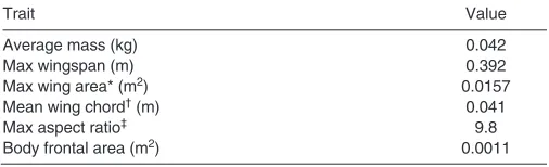
The length from the beak to a white marker on the rump of the bird was measured on images of the bird held next to a reference grid to be used as reference length for accurate pixels-to-meters conversion of high-speed films (see below). Also, from these reference images of the hand held bird, the projected area of the head and the distance between the eyes were measured. These measures were used to test the accuracy of the scale determined, based on the beak-to-marker reference length in each of the image frames of the high-speed films (see below). The maximum wing area and wingspan was also measured on the hand held bird with fully spread wing according to the method in Fig.2. The morphological details of the bird are presented in Table1. On 6th September 2009 the birds were released into the wild in good condition.

Wind tunnel

The Lund wind tunnel has a closed circuit design with an open test section. The design is customized for experiments with freely flying animals. The background turbulence is low, approximately 0.03% (Spedding et al., 2009) and airspeed across 97% of the test section is within ±1.3% of the mean (Pennycuick et al., 1997). Details on –mg

L=mgcos_θ

Us U

D=mgsinθ

θ θ

mg

Fig.1. Forces acting on the swift in equilibrium gliding. The glide path is

inclined at an angle to the horizontal and the resultant of the vectors lift

(L) and drag (D) is equal and opposite to the weight of the bird (mg). Total

speed (U) involves the velocity component sink speed (Us), which is

directed downwards and perpendicular to the horizontal.

Sw St

bw

bt

Fig.2. Body and wing outline of a swift. The grey-colored areas show how

wing area (Sw) and tail area (St) was measured from top-view high-speed

film sequences of the bird during steady gliding. Dashed lines show

definition of wingspan (bw) and tail span (bt). The distance from the beak to

the design and specifications of the wind tunnel are presented in Pennycuick et al. (Pennycuick et al., 1997). The Reynolds number, calculated as ReUc/, where cis the mean chord of the wing and

is the kinematic viscosity, ranged from approximately 18400 at 7ms–1_{to 29500 at 11ms}–1_{. The coordinate system for the tunnel} is defined as: x-axis: streamwise, y-axis: spanwise and z-axis: vertical.

Experimental setup

The wing morphology during flight was recorded with a high speed camera (NAC Hotshot 1280, Simi Valley, CA, USA; 1280pixels⫻1024pixels) filming the bird straight from above. The wake was sampled using stereo digital particle image velocimetry (SDPIV) at a plane transverse (y,z) to the free stream flow. The imaging plane was approx. 0.3–0.4m (8–11 wing chord lengths) downstream of the bird. The SDPIV and the high-speed camera were triggered when the bird was gliding steadily in the appropriate position. The high-speed camera was, during the DPIV experiments, used also to record the location of the bird relative to the imaging plane and the flight behavior of the bird.

Experimental protocol

The bird was allowed to fly freely in the wind tunnel and it was not guided by any means. The bird was flown at five different flight speeds: 7, 8, 9, 10 and 11ms–1_{. For each speed, the tunnel was} initially tilted to its maximum, 6.3deg, and then tilted back towards horizontal in increments of 0.1deg until the bird was just able to glide steadily. This angle corresponds to the minimum decent angle for that particular speed. Once the angle was found the procedure was repeated from the 6.3deg position with a new speed. At all speeds it was clear when the minimum angle was found because the bird would not be able to glide steadily at any lower angle, but would either descend or decelerate. For the wake measurements each of the speeds and corresponding minimum tilt angles were revisited and thereby the previous measurements were confirmed. The bird was at all speeds able to glide steadily at all angles steeper than the minimum.

High-speed camera details

The high-speed camera was mounted on top of the test section and thereby always perpendicular to the airflow regardless of the tunnel tilt angle. The camera was triggered manually and captured the bird for 0.75s at 250f.p.s. From each of the recorded sequences, a single frame was used to measure wing area, tail area, wingspan and tail span with Scion Image (Scion Corporation, www.scioncorp.com; see Fig.2) using the reference lengths and area described above. The frames were taken only from steady gliding sequences. Images from two to three sequences per angle and speed combination were analyzed and the average was calculated.

DPIV details

Flow field areas of approximately 0.20m⫻0.20m were recorded using two CMOS-sensor cameras (High-SpeedStar3, LaVision, Goettingen, Germany: 1024pixels⫻1024pixels) connected to frame grabber PCI boards in a host computer. The cameras were equipped with 60mm lenses (AF Micro Nikkor 60mm f/2.8D) set to aperture 2.8. A thin fog (particle size 1m) was introduced into the tunnel downstream from the test section and circulated in the tunnel until even. The fog particles were illuminated by a pulsed 50mJ laser (Litron LPY732 series, Litron Lasers, Rugby, UK; Nd:YAG, 532nm) generating pulse pairs at 200Hz repetition rate. The laser beams were spread by a cylindrical lens into a thin sheet covering the view of the two cameras. To filter out light from any other source than the laser the cameras were equipped with band pass filters (530±5nm). The system was operated using DaVis 7.2.2 software package (LaVision). The DPIV cameras were calibrated using a calibration plate (0.20m⫻0.20m; type 22) and the routine in DaVis. The calibration was fine tuned using the self-calibration routine in DaVis, by which any misalignment between the laser sheet and calibration plate is corrected.

The DPIV data were analyzed using DaVis software. The raw images were pre-processed prior to vector computations by using subtract-sliding-minimum filter over five frames. For image correlation, multi-pass stereo cross correlation was used (64⫻64 in initial step and 32⫻32 in final step, 50% overlap). Vectors in the resulting vector field showing peak ratios <1.01, when dividing the highest correlation peak with the second highest correlation peak, were deleted. Vectors were also deleted if the magnitude was two times the neighborhood rank mean squares (RMS) and recalculated if the magnitude was three times the neighborhood RMS. As a final post-processing stage, empty spaces were interpolated and a 3⫻3 smoothing average was applied. For each sequence, background velocity measured on free stream flow was subtracted from the out of plane velocity. DPIV sequences were only used for further analysis if they corresponded to high speed film sequences showing the bird in steady gliding.

Wake measurements

Vortex circulation and estimate of lift

The processed wake images were used for calculating the circulation () of identifiable wake structures. This was done for each minimum glide angle at each speed. The wake of the gliding swift consists mainly of a pair of wingtip vortices and a pair of tail vortices (see below). Circulation was measured using a custom written Matlab program (The MathWorks, Inc., Natick, MA, USA) and otherwise following the same procedure as described by Spedding et al. (Spedding et al., 2003). Averages over all sequences for each speed were calculated for wingtip vortices and tail vortices, respectively. According to lifting line theory and the Kutta–Joukowski theorem the force generated by a fixed finite wing can be approximated by:

L bw,wakeU, (10)

where bw,wakeis wake span and is circulation. Both the wingtip and tail vortices were assumed to contribute to lift and hence total lift generated by the gliding swift was calculated as:

L U (bw,wakew+ bt,waket) , (11)

where bw,wake is represented by the average wingtip vortex wake span, wis average circulation of the wingtip vortex, bt,wakeis the average tail vortex wake span and tis average circulation of the tail vortex. Since the DPIV cameras, the laser sheet, and consequently the orientation of the recorded image plane, follow Table 1. Morphological details of the bird used in the experiments

Trait Value

Average mass (kg) 0.042

Max wingspan (m) 0.392

Max wing area* (m2_{) 0.0157}

Mean wing chord†_{(m) 0.041}

Max aspect ratio‡ _9.8

Body frontal area (m2_{) 0.0011}

*Area of both wings including the body area in between. †_{Wing area divided}

the tilt of the tunnel, the calculated lift will correspond to the lift generated by the bird (mgcos; see Fig.1) and not the weight of the bird (mg) at any given glide angle (; see Fig.1).

Velocity defect and estimate of parasite drag

In order to estimate the drag generated by the body alone [parasite drag (e.g. Pennycuick, 1989; Pennycuick, 2008)], the out-of-plane (x) velocity defect behind the body was measured. When plotting the streamwise velocity of the complete frame the deceleration of the freestream airflow introduced by the bird could be distinguished (cf. Hedenström et al., 2009). Patches of decelerated flow were typically found in the wingtip vortices, the tail vortices and behind the body (Fig.3A). To estimate the drag by the body alone the air velocities were measured in the location of the body, but excluding the drag introduced by the tail vortices (Fig.3A). These measurements were performed using a custom written Matlab program, which allows the user to manually define an area of interest containing the velocity defect created by the body. Within this area the streamwise velocities of vectors having a velocity less than 20% of the freestream flow were measured. From this the mass flow rate was calculated as:

m A Ub, (12)

where Ais the measured wake area and Ubis the airspeed behind the body. Parasite drag was then calculated as:

Dpar|m DU| , (13)

where DUis the difference in airspeed between the decelerated air behind the body (Ub), and the unaffected freestream flow, U⬁.

Finally, the body drag coefficient was calculated as:

where Sbis the body frontal area of the bird (Table1).

Measurement errors

All measurements are associated with some uncertainty, which is usually expressed as a proportion of the quantity in question. For a function of two independent variables f(x1, x2), the uncertainty Df

is calculated as:

The estimation of lift to drag ratio, either as based on the steady gliding flight in a tilted wind tunnel or as extracted from wake properties using flow visualization, is based on composite functions including multiple parameters, each of which has an uncertainty when measured or estimated. To illustrate we assess the uncertainty of estimating the lift to drag ratio (L:D) based on a gliding bird in a tilted wind tunnel (see above). The criterion is that the bird must be in steady gliding flight, which means that the bird is not moving with respect to the wind tunnel frame of reference (but moves in relation to the air). L:Dis given by U/Us, where Uis the forward gliding speed and Usis the vertical component of the speed (sink speed). Uis set as wind tunnel speed, with an estimated uncertainty of 0.05ms–1_{, so at a speed of 10ms}–1_{, the relative uncertainty}

DU/U is 0.005 (0.5%). The tilt angle is selected with an uncertainty 0.02deg, and so the sink speed is determined from Us

Usin. Hence, DUs[(DUsin)2+(DUcos)2]1/2{[0.05sin(4.46)]2+ [0.02cos(4.46)]2_}1/2_{0.02, using example values U9.0±0.05ms}–1_,

4.46±0.02deg.

CD,par =_ρ2_UD₂par_S b

, (14)

∂f

∂x1 Δx1 ⎛ ⎝⎜

⎞ ⎠⎟ 2

+ ∂f ∂x2

Δx2 ⎛ ⎝⎜

⎞ ⎠⎟ 2 ⎧

⎨ ⎪ ⎩⎪

⎫ ⎬ ⎪ ⎭⎪ 1/2

. (15)

U is determined with the uncertainty of 0.05ms–1_{, which at}

U9ms–1_{gives the relative uncertainty DU/U0.05/90.006. Hence,}

Wingtip

Body

Tail

+ –

Wingtip

Tail

−200 0 200

+ –

B

A

6 9 12

Fig.3. An example of velocity vector fields superimposed on (A)

out-of-plane velocities and (B) vorticity at 9ms–1_{, illustrating how the velocity}

determining the L/Dratio from the gliding path as determined by the minimum gliding angle for steady flight, using the same method as above, is associated with an uncertainty of approximately 0.03. For calculating the lift based on vortex wake measurements we use the relationship LY. The composite uncertainty is straightforward in this case DL[(YD)2_+(YDb)2₊ (bYD)2+(bDY)2_]1/2_{, so for typical values of this experiment} (1.20±0.005kgm–3_{, b0.39±0.005m, 0.055±0.0055m}2_s–1_,

U9.0±0.05ms–1_{) DL/L evaluates to 0.06. This means that the} uncertainty in wake-based lift is less than or about 6%.

Details on the performance of the PIV system can be found in Stanislas et al. (Stanislas et al., 2008).

RESULTS

Gliding flight characteristics

Only one of the two birds that were initially tested would glide in the tunnel. This bird only glided for brief periods on the first day and not very steadily, but the second day the bird appeared to have learned how to utilize the opportunity for gliding flight and started to glide steadily for longer periods. The bird would not glide unless the tunnel was tilted, but would glide at all tilt angles steeper than the minimum angle. The bird was able to glide steadily at speeds in the range from 7 to 11ms–1_{. At the lower speeds the gliding} events were rarer and shorter in duration than at higher speeds. The higher speeds were clearly more suitable for the swift, although the highest speed, 11ms–1_{, seemed challenging for the bird in terms of} maneuvering with respect to the wind tunnel walls. The typical behavior of the bird was to accelerate flapping flight upstream into the centre of the test section, then switch to gliding flight, and depending on the speed and tilt angle, it would remain stationary with respect to the test section from a couple of seconds up to approximately 10s.

Wing and tail morphology

Wingspan, wing area, span ratio and aspect ratio are measures of the wing morphology of a gliding bird. By measuring these variables over a range of flight and sink speeds the dynamic morphing of the bird wing can be roughly described.

The swift changed its wing morphology to a large extent between different speeds and glide angles. The span ratio, defined as the ratio between observed wingspan (bw,obs) and maximum span (bw,max); hand held bird with manually spread wing; see Table1), decreased linearly with speed, from approximately 0.9 at 7ms–1 _{to 0.85 at 11ms}–1_{, although with a large scatter} (Fig.4A). This reduction in wingspan was achieved by the bird mainly by flexing the wing at the wrist joint and thus sweeping the wing backwards. The wing area was reduced linearly with reduced span, from 0.016m2 _{(99.0% of maximum area) at the}

widest span measured, 0.39m (99.7% of maximum span) to

0.011m2_{(70.9% of maximum area) at the shortest span measured,} 0.30m (77.2% of maximum span; Fig.5). Fig.5 shows this relationship independent of speed.

The mean chord (c) of the wing is defined as wing area/wingspan. The mean chord of the swift decreased with flight speed, with respect

Me a n c hor d, c (m)

6 7 8 9 10 11 12 Airspeed, U (m s–1₎

T a il s p a n, bt (m) bw, o bs / bw, m a x 0.6 0.65 0.7 0.75 0.8

0.85 0.9 0.95 1 1.05

0.03

0.032 0.034 0.036 0.038 0.04 0.042 0.044 0 0.01 0.02 0.03 0.04 0.05 0.06 0.07 0.08 0.09 0.1

C

B

A

Fig.4. (A)Span ratio (bw,obs/bw,max) in relation to flight speed. Filled circles

represent the complete data including all combinations of speed and tilt angles, and open circles represent the minimum tilt angle for each speed. The solid line shows the linear regression function for the

complete data (bw,obs/bw,max–0.0123U+0.9865; R20.13) and the broken

line shows the linear regression function for data points corresponding to

minimum tilt angle (bw,obs/bw,max–0.0139U+1.0115; R20.66). (B)Mean

chord (c) in relation to airspeed. Filled circles represent all speed–angle

combinations (c–0.001U+0.048, R2_{0.48) and open circles represent}

the minimum tilt angle for each speed (c–0.0006U+0.044, R2_{0.75). The}

solid line shows the regression line fitted to the complete data set, and the broken line shows the regression line fitted to the minimum tilt

angles. (C)Tail span (bt) as a function of speed. The tail is more spread

at the lowest speed, 7ms–1_{. At all other speeds the tail is kept furled}

together to a large extent, and at the highest speed, 11ms–1_{, the tail is}

completely furled.

0.7 0.75

0.8

0.85

0.9 0.95 1

0.77 0.82 0.87 0.92 0.97

Wingspan ratio

W ing a re a r a tio 0.011 0.0115 0.012 0.0125 0.013

0.0135

0.014 0.0145 0.015 0.0155

0.3015 0.3215 0.3415 0.3615 0.3815

Wingspan (m)

W ing a re a (m 2)

Fig.5. Wing area (Sw) as a function of wingspan (bw) presented in absolute

measures and as a ratio of the maximum values (denoted with *). There is a linear positive relationship between wingspan and wing area. Regression

for span ratio: S*1.28bw*–0.2785, R20.68 regression for absolute

to both all speed–angle combinations and minimum tilt angle for each speed (Fig.4B).

The tail span decreased with speed from 0.09m at 7ms–1_{to 0.04} at 11ms–1_{. The tail was spread notably more at 7ms}–1_{than at any} of the other speeds (Fig.4C).

Flight performance

Sink speed

The sink speed (Us) of the bird, i.e. the vertical component of the total flight speed, was calculated for the cases of minimum tilt angle of the wind tunnel for each flight speed. The sink speed showed a curvilinear relationship with speed. Fitting a second order polynomial regression equation to the data yields the relationship

Us0.032U2–0.51U+2.76 (Fig.6A; R20.96). Minimum sink speed (Ums) as estimated by the speed at the minimum of this equation was Ums8.1ms–1. If a tangent is drawn from the origin towards the curve, the speed at the intercept corresponds to the best glide speed (Ubg), which is estimated to Ubg9.4ms–1(Fig.6A).

Lift and drag

Lift and drag were calculated based on the weight of the bird and the tilt angle of the wind tunnel, i.e. the angle of descent of the glide path, according to Eqns2 and 3. Drag was further broken down into induced drag (Dind), parasite drag (Dpar) and profile drag (Dpro). Induced drag was calculated according to Eqn6, using an induced drag factor (k) of 1.1, parasite drag was estimated from the wake (see below) and profile drag was calculated according to Eqn7. Total drag showed a curvilinear relationship with speed (D0.0016U2_{–0.030U+0.18; R}2_{0.95) with a minimum at 9.4ms}–1_. Induced drag decreased with speed (Dind0.0020U+0.039; R20.96). Profile drag showed a shallow U-shaped relationship with speed

(Dpro0.0013U2–0.025U+0.13; R20.96), with a minimum at 9.6ms–1_{, and parasite drag increased with speed (D}

par 0.0019U–0.0039; R2_{0.99; Fig.6B).}

The speed-specific maximum ratio of lift to drag (L:D) showed an inversely quadratic relationship with airspeed (L:D–0.48U2_{+9.2U+31; R}2_{0.94; Fig.6C). The maximum of the} second order polynomial regression equation was used to estimate the maximum L:D, which was 12.5. This maximum was reached at a flight speed of 9.5ms–1_{(although the maximum L:Dmeasured} was 12.7 at 10ms–1_).

The coefficient of lift (CL) was calculated at the minimum glide angle for each speed according to Eqn8, using the measured wing area or the sum of the wing area and tail area. The lift coefficient decreased from 0.96 at 7ms–1 _{to 0.48 at 11ms}–1 (CL0.015U2–0.40U+3.04; R20.99) with wing area as reference, and from 0.81 at 7ms–1_{to 0.43 at 11ms}–1_(C

L0.010U2–0.28U+2.3;

R2_{0.99) with the sum of wing and tail area as reference (Fig.7A).} The highest CL measured here is not necessarily the maximum attainable for the bird. The maximum tilt angle of the tunnel is 6.3deg. and with an even steeper tilt angle the true maximum CL may be higher. Analogously, the minimum speed, or stall speed, may be slower than the minimum speed measured here, 7ms–1_. Coefficient of total drag (CD) was calculated, similarly to CL, for the minimum glide angle of each speed according to Eqn9. The coefficient of drag decreased non-linearly from 0.1 at 7ms–1_{to 0.043} at 11ms–1_(C

D0.0044U2–0.095U+0.54; R20.99) with wing area as reference and from 0.084 at 7ms–1 _{to 0.038 at 11ms}–1 (CD0.0035U2–0.075U+0.44; R20.99) with the sum of wing and tail area as reference. Both curves flatten out between 10ms–1_and 11ms–1_(Fig.7B).

Profile drag coefficient was calculated similarly to the total drag coefficient (cf. Eqn9) for all speed and tilt angle combinations. Plotting CD,proagainst CLgives the polar area [terminology from Tucker (Tucker, 1987)], which describes the relationship between

CD,proand CLfor the morphing swift wing (Fig.8). Minimum CD,pro was 0.011 and was found at 10ms–1_.

0 0.2 0.4 0.6 0.8

1 1.2

S

in

k

s

peed,

Us

(m

s

–1

)

0 0.005 0.01 0.015 0.02 0.025 0.03

0.035 0.04 0.045 0.05

Dr

a

g (

N

)

8

9 10 11 12 13

14

6 7 8 9 10 11 12

0 2 4 6 8 10 12

L

:

D

Airspeed, U (m s–1₎

C

B

A

Fig.6. (A)Sink speed in relation to airspeed. Filled circles show all

speed–angle combinations with the lowest sink speed for each speed encircled. The relationship between speed and lowest sink speed can be described with a second order regression polynomial:

Us0.0315U2–0.5101U+2.7588, R20.961. The speed at the minimum of

this equation corresponds to the speed of minimum sink; Ums8.1ms–1. If a

tangent is drawn from the origin towards the curve (Us0.0795U), the

speed at the intercept corresponds to the best glide speed, Ubg9.4ms–11.

(B)Drag as a function of airspeed. Filled circles represent total drag with

the lowest drag encircled, squares represent induced drag, triangles represent profile/parasite drag and open circles represent profile drag

alone. Total drag has a minimum at 9.44ms–1_{. Induced drag decreased}

with airspeed and the combined profile and parasite drag showed a

U-shaped curve with a minimum at 8.54ms–1_{. (C)}_{Lift to drag ratio (L:D) as a}

function of airspeed. Maximum L:D (encircled dots) showed a curvilinear

relationship with airspeed (L:D–0.4849U2_{+9.2059U+31.204, R}2_0.9376),

Wake topology

The wake of the gliding swift consists of two main structural parts: a pair of wingtip vortices and a pair of tail vortices. Fig.9 shows characteristic images of the vector and vorticity fields at 7ms–1_, 9ms–1_{and 11ms}–1_{that visualize the trailing wingtip vortex of the} left wing and both tail vortices. The wingtip vortex is similar at all speeds, but the tail vortices differ. At 7ms–1_{the tail vortices are far} apart as a consequence of the widely spread tail, whereas at 9ms–1 and 11ms–1_{the tail vortices are gradually closer together. The same} pattern emerges when plotting the tail span measured on the bird in flight against speed (see Fig.4C).

Images from one high-speed SDPIV sequence of 9ms–1_gliding flight were compiled into a three-dimensional wake representation by translating the time delay between the images (Dt1/200s) into spatial displacement (DxDtU⬁), assuming a constant convection

contributed by the freestream flow (U⬁) alone. The compiled

three-dimensional image was used to plot the vorticity iso-surface of the wake (Fig.10). The iso-surface plot shows the normalized constant streamwise vorticity (iso-value80s–1_{) trailing behind the gliding} bird.

Quantitative wake measurement

Wingtip circulation, tail circulation and lift

The main features of the wake of the gliding swift are the wingtip vortices and the tail vortices (Fig.10). Circulation () of these structures was measured for each sequence and the average was calculated (Fig.11). The circulation of the wingtip vortices decreases

in strength with increasing speed, whereas the tail vortices vary with speed without any apparent trend.

Lift was calculated according to Eqn11 for each flight speed. The model involved wingtip vortices and tail vortices as these were assumed to result from lift generation. The model is described conceptually in Fig.12.

Total lift calculated from the wake-based model showed good agreement with the lift calculated using the glide angle of the flight path (Fig.13A). The lift calculated with the model was 105%, 98%, 101%, 101% and 105% of the lift calculated using the glide angle of the bird for 7, 8, 9, 10 and 11ms–1_{, respectively.}

Body wake defect and estimate of parasite drag

The estimate of body drag was an attempt to distinguish this from the total drag of the bird. The calculated body drag, or parasite drag, increased with speed from 0.0097N at 7ms–1_{to 0.0172N at 11ms}–1 (Fig.13B). In proportion to the calculated total drag based on glide angle this estimated drag of the body varies from 23% at 7ms–1_to 46% at 11ms–1_{. The parasite drag coefficient, calculated according} to Eqn14, decreases from 0.30 at 7ms–1_{to 0.22 at 11ms}–1_{(Fig.13C).}

DISCUSSION Flight behavior

The swift turned out to be a skillful glider in the wind tunnel. This was perhaps not surprising, since these birds glide for a considerable proportion of the time in the wild (Lentink et al., 2007; Henningsson et al., 2009). By contrast, it was surprising that one bird never started to glide properly and it took the other bird a couple of days before it began exploring the opportunity for gliding flight in the tunnel. Once the single bird had started to explore gliding flight it soon started to glide for relatively long periods. The bird would glide at any tilt angle lower or equal to the lowest possible for each speed. The stability of the glides could vary, typically the glides would be shorter at very high and at very low tilt angles. When approaching the lowest angle the glides would typically become shorter and the bird would also glide less frequently, suggesting that it was at its performance limit. The range of flight speeds that the swift would glide at was rather limited, 7–11ms–1_{, although this range is similar} to that recorded previously for flapping flight in a wind tunnel (Henningsson et al., 2008), and 11ms–1 _{is the highest speed} recorded for any swift in the tunnel.

0.3

0.4 0.5 0.6 0.7 0.8

0.9 1 1.1 1.2

0 0.01 0.02 0.03 0.04 0.05 0.06

CL

CD,pro

Fig.8. Polar area for the wings of the swift gliding at equilibrium for all

airspeed and tilt angle combinations examined. Outline circles represent minimum tilt angle and outline squares represent the maximum tilt angle.

CL, coefficient of lift; CD,pro, profile drag coefficient.

0 0.2 0.4 0.6 0.8

1 1.2

CL

0 0.02 0.04 0.06 0.08

0.1 0.12

6 7 8 9 10 11 12

CD

Airspeed, U (m s–1₎

B

A

Fig.7. Coefficient of lift (CL) and drag (CD) at minimum tilt angle as a

function of airspeed. Circles represent coefficients calculated using only wing area as the reference area; squares represent coefficients calculated using the combined area of the wings and tail as the reference area.

(A)Second order polynomial regression for coefficient based on wing area

alone: CL0.0154U2–0.4031U+3.0377, R20.99, and for joint wing area and

tail area: CL0.0101U2–0.2827U+2.3095, R20.99. (B)Coefficient of drag

decreases with flight speed but levels out within the measured range.

Second order polynomial regression for CDbased on wing area alone:

CD0.0044U2–0.0946U+0.5449, R20.99, and for combined wing area and

Flight performance

The highest coefficients of lift measured for the swift was 0.96, or 0.81 if excluding or including the tail area in the calculation (Fig.7A). Lentink et al. (Lentink et al., 2007) examined the glide performance of swifts by measuring lift and drag of preserved wings. They found a CLbetween 0.8 and 1.1, which is in good agreement with the results presented here for a live bird. The CLof the swift can also be compared with that of a jackdaw [Corvus monedula

(Rosén and Hedenström, 2001)], a pigeon [Columba livia

(Pennycuick, 1968)], a Harris’ hawk [Parabuteo unicinctu (Tucker and Heine, 1990)] and a laggar falcon [Falco jugger(Tucker and

Parrot, 1970; Tucker, 1987); Table2]. Apart from the pigeon, these species are all raptors, more or less adapted for soaring flight. The swifts are, in their ecology and morphology unlike most birds; they are aerial insectivores and have quite unique wing morphology, with a very long hand section and a short arm section. The maximum

CLfor the swift was the same as for the pigeon, but lower than in the soaring specialists (Table2). This could reflect diverging adaptations of the wing design between these birds, where a high

CLis required for minimum turn radius when circling in thermals and during take-off and landing. The maximum L:Dwas similar in the swift to the maximum of the other species (Table2). The larger Wingtip

Tail

Wingtip

Tail

−200 0 200

+ –

Wingtip

Tail

A

C

B

Fig.9. Example images of the vector and vorticity fields at (A) 7ms–1_{, (B) 9}_m_s–1_{and (C) 11}_m_s–1_{. The wingtip vortex is similar at all speeds, but the tail}

soaring specialists, except the laggar falcon, have separated primaries to generate a slotted wingtip. Slotted wingtips have been shown to reduce induced drag by vertical spreading of the vortices shed at the wingtip (Tucker, 1993), and so they appear to achieve a high

L:Dby minimizing drag. The swift does not have wingtip slots, but achieves the relatively favorable L:Dby having relatively long wings (high aspect ratio; Table2) that reduces the induced drag.

The drag as calculated, based on the glide angle of the bird, represents the drag of the whole configuration. This includes several parts, among which the induced drag was estimated from theory. A similar approach was used by Rosén and Hedenström (Rosén and Hedenström, 2001) on the jackdaw. In that study an estimate of combined profile and parasite drag was derived by subtracting the induced drag from the total drag. If summarizing profile and parasite drag for the swift, an interesting feature is that the induced drag is

lower than the profile and parasite drag, whereas these components were opposite for the jackdaw. The low induced drag for the swift compared with the jackdaw can be explained if, for illustrative purposes, Eqn6 is rearranged:

where W/S(weight/area) is the wing loading and ARis the aspect ratio of the wing. The wing loading for the swift was 26kgm–2_and for the jackdaw it was 30kgm–2_{(Rosén and Hedenström, 2001).} The aspect ratio for the swift was 9.8, and 6 for the jackdaw. Thus, for any given speed, the numerator will be lower and denominator will be higher for the swift compared with the jackdaw, both resulting in a lower Dind.

Gliding wake and forces estimated from it

The wake of the gliding swift is comparatively simple. The main features are a pair of wingtip vortices and a pair of tail vortices. Spedding studied the wake of a kestrel (Falco tinnunculus) in gliding flight (Spedding, 1987). In that study only the wingtip vortices were apparent, while the tail vortices were not observed and therefore not included in the model developed to describe the wake. In the wake of the swift the tail vortices are prominent features, in fact, the circulation of the tail vortices is sometimes nearly as high as that of the wingtip vortices. However, despite the high circulation of the tail vortices the effective contribution to the total lift is small in comparison with the wingtip vortices, because of the small span of the tail (recall Eqns10 and 11).

The model of the wake of the gliding swift, proposed here, and the estimated forces showed reasonable agreement with the lift calculated using the glide angle of the bird. This model includes wingtip vortices and tail vortices, and the circulation measured in the wake is assumed to directly reflect the circulation of the lift generating bound vortex. This is assumed to be a simplified view, since it does not take into account the circulation distribution on

Dind= 2kS W

S

⎛ ⎝ ⎜⎜ ⎞_⎠⎟⎟

2

ρπU2_AR , (16)

Fig.10. Vorticity iso-surface plot at an airspeed of 9ms–1_{. The view is}

obliquely from above and from the front of the bird’s flight path, as indicated by the bird silhouette. The plot is based on data from one side of the bird, wing and tail, that have been mirrored in the plot to illustrate the complete wake. Tail vortices and wingtip vortices are the major structures in the wake of the gliding swift and appear clearly in this plot.

0 0.01 0.02 0.03

0.04 0.05 0.06 0.07

6 7 8 9 10 11 12

Γ

Airspeed, U (m s–1₎

Fig.11. Circulation () as a function of airspeed. Filled circles represent

wingtip circulation and open circles represent tail circulation. Wingtip circulation decreases with speed, whereas tail circulation shows no apparent relationship with speed. At several speeds the circulation of the tail is of the same order as that of the wingtip.

Γw

Γw

Γt

Γt

bw 2

bt 2

bt 2

bw 2

Fig.12. Illustration of the wake-based model consisting of a pair of trailing

the wing and assumes no convection in the wake other than that of the freestream flow. The model is based on the measured wake span and not the span of the bird, which means that it takes into account

the contraction of the wake (e.g. Milne-Thompson, 1966), but other than that it is assumed that the wake is unaffected as it travels downstream of the bird. The fact that the model, despite its simplicity, matches the expected force to such a large extent, suggests that the wake of a gliding bird is indeed simple.

A model of the wake of a gliding swift has previously been proposed by Videler et al. (Videler et al., 2004). In that study a brass model of a swift wing was examined in a water tunnel. The results showed stable leading edge vortices originating from the inner section of the wings, extending out across the wings and merging with the wingtip vortices. The measurements by Videler et al. were taken on the wing, whereas the measurements in the present study were taken in the far wake, which makes the two studies not fully comparable. However, there is nothing found in the wake topology in this study that rules out the existence of a leading edge vortex on the wing, but equally, there is nothing obvious to support the model either.

As mentioned above, the drag, calculated using glide angle, represents the total drag. Since the system for flow visualization used also gives the out-of-plane (x) velocities, an attempt was made to estimate the drag of the body (parasite drag) from the drag of the whole bird, based on the wake defect. The results showed that the drag coefficient of the body ranged from 0.30 at 7ms–1_{to 0.22} at 11ms–1_{. Note that this coefficient is not directly comparable with} the total coefficient of drag calculated here, since the characteristic area used for the total drag coefficient was the wing area, whereas for the body drag coefficient the body frontal area was used (Pennycuick, 2008). Drag coefficients of zebra finches (Taeniopygia guttataVieillot) in bounding flight, with wings completely folded, were estimated as 0.5 at 10ms–1_{and higher still at slower speeds} (Tobalske et al., 2009). These values are not directly comparable with those of the gliding swift, because the zebra finches exhibit a body angle of attack to generate lift, which causes increased parasite drag. A comparable body drag coefficient of the swift body was estimated by Lentink et al. (Lentink et al., 2007) by measuring the drag of a taxidermically prepared wingless swift body using an aerodynamic balance. In that study the body drag coefficient was found to be on average 0.26. The range measured here includes this value with an average over all speeds of 0.26. Measuring drag on dead whole or stuffed bird bodies has been proposed to result in an overestimate compared with the true drag generated by a live bird in flight (Tucker, 1973; Pennycuick et al., 1988) (but see Hedenström and Liechti, 2001). The results of this study suggest that this is not necessarily the case under all circumstances.

Profile drag could be estimated in this study since the induced drag could be calculated and the parasite drag could be measured. This is, as mentioned, the most difficult aerodynamic component to measure (Pennycuick, 1989; Pennycuick, 2008), although, it has been done a few times before on live birds. Tucker and Heine (Tucker and Heine, 1990) studied a Harris’ hawk gliding in a wind tunnel with a similar approach as in the present study. In that study profile drag was estimated, similar to this study, by subtracting 0

0.05 0.1 0.15 0.2 0.25 0.3

0.35 0.4 0.45 0.5

Li

ft (

N

)

0 0.002 0.004 0.006 0.008

0.01 0.012 0.014 0.016 0.018

0.02

Dp

a

r

(N)

0 0.05 0.1 0.15 0.2 0.25 0.3

0.35 0.4

6 7 8 9 10 11 12

CD,

p

a

r

Airspeed, U (m s–1₎

C

B

A

Table 2. Data for five bird species compiled from literature

Species Mass (g) Wingspan (m) Aspect ratio Ums(ms–1) Ubg(ms–1) Max L:D CL

Harris’ hawk* 0.702 1.02 5.5 8.8 12.0 10.9 1.60

Jackdaw† _{0.180 0.60 6.1 7.4 8.3 12.6 1.49}

Laggar falcon‡ _{0.570 1.01 7.7 9.0 11.3 10 1.60}

Pigeon§ _{– 0.67 6.0 – – 12.5 0.96}

Swift¶ _{0.042 0.39 9.8 8.1 9.4 12.5 0.96}

Ums, airspeed of minimum sink; Ubg, airspeed of best glide; Max L:D, maximum lift to drag ratio; CL, coefficient of lift.

*Tucker and Heine, 1990. †_{Rosén and Hedenström, 2001.} ‡_{Tucker and Parrot,1970; Tucker, 1987.} §_{Pennycuick,1968.} ¶_{The present study.}

Fig.13. (A)Lift as a function of airspeed. Filled circles represent lift

generated by the wingtip vortices and open circles represent lift generated by the tail vortices. Squares represent the sum of lift measured in the wake

and triangles represent the lift calculated based on glide angle. (B)Parasite

drag (Dpar) in relation to airspeed. Drag of the body, as a fraction of the

total drag estimated based on the glide angle of the bird, decreased from

23% at 7ms–1_{to 46% at 11}_m_s–1_{. (C)}_{Parasite drag coefficient (C}

D,par) in

induced drag and parasite drag from the measured total drag to yield the profile drag coefficient, CD,pro. However, Tucker and Heine (Tucker and Heine, 1990) calculated parasite drag based on equivalent flat plate area. The same Harris’ hawk was used by Pennycuick et al. (Pennycuick et al., 1992) to estimate the profile drag by measuring the pressure of the air behind the wing. The results from these two approaches of estimating profile drag of the same bird differed: Tucker and Heine (Tucker and Heine, 1990) found a range of CD,pro from 0.003 to 0.097, whereas Pennycuick et al. (Pennycuick et al., 1992) found a range from 0.008 to 0.052. In the present study of the swift the range of CD,prowas from 0.011 to 0.048. The lower end is higher for the swift than the lower end for the Harris’ hawk, whereas the upper end is lower for the swift than the upper end for the Harris’ hawk. The shape of the polar area of the swift is similar to that of the Harris’ hawk as described by Tucker and Heine, whereas the shape of the polar area found by Pennycuick et al. for the Harris’ hawk differed (Tucker and Heine, 1990; Pennycuick et al., 1992). In such polar plots, the left-hand side of the polar area boundary represents the polar curve for minimum drag, whereas the right-hand side of it represents the polar curve for maximum drag. This maximum drag polar does not correspond to the maximum drag polar curve possible for the bird unless the wings stalls (Tucker and Heine, 1990). There were no signs that the wings of the swift were stalling at any occasion during the experiments, i.e. no lifted coverts or irregular fluttering, so it is likely that the right-hand boundary in the polar area does not fully represent the true maximum drag polar for the swift. However, as can be seen in Fig.8, CD,profor the maximum tilt are all found along the right-hand boundary, suggesting that the bird is maintaining equilibrium gliding by braking with the wings, i.e. adding to the total drag. Furthermore, CD,profor minimum tilt angle are all located along the left-side boundary, which is expected if the bird, on these occasions, adjusts its wing shape to minimize drag.

LIST OF SYMBOLS AND ABBREVIATIONS

A measured wake area behind body

AR wing aspect ratio

bw wingspan bt tail span bt,wake tail wake span bw,max maximum wingspan bw,obs observed wingspan bw,wake wing wake span c mean wing chord

CD drag coefficient CD,par parasite drag coefficient CD,pro profile drag coefficient CL lift coefficient D drag

Dind induced drag Dpar parasite drag Dpro profile drag

g gravitational acceleration

k induced drag factor

L lift

m mass flow rate

m mass of the bird

Re Reynolds number

Sb body frontal area Sw wing area U airspeed

U_⬁ freestream flow

Ub airspeed behind body Ubg airspeed of best glide Ums airspeed of minimum sink Us sink speed

Utrue true airspeed W weight of the bird

 circulation

w average circulation of the wingtip vortex t average circulation of the tail vortex  glide angle relative to horizontal

 kinematic viscosity

 air density

ACKNOWLEDGEMENTS

We thank Jan Holmgren for providing the two juvenile swifts. We also wish to thank Teresa Kullberg for invaluable help during the experiments. We are grateful to Christoffer Johansson and Florian Muijres for developing the analysis software for the wake data and for suggestions and ideas on the project, as well as help with experimental setup. This study was supported financially by grants from the Swedish Research Council and the Knut and Alice Wallenberg Foundation. A.H. is a Royal Swedish Academy of Science Research Fellow supported by grants from the Knut and Alice Wallenberg Foundation.

REFERENCES

Hedenström, A. and Liechti, F.(2001). Field estimates of body drag coefficient on the basis of dives in passerine birds. J. Exp. Biol. 204, 1167-1175.

Hedenström, A., van Griethuijsen, L., Rosén, M. and Spedding, G. R.(2006). Vortex wakes of birds: recent developments using digital particle image velocimetry in a wind tunnel. Animal Biol. 56, 535-549.

Hedenström, A., Johansson, L. C., Wolf, M., von Busse, R., Winter, Y. and Spedding, G. R.(2007). Bat flight generates complex aerodynamic tracks. Science

316, 894-897.

Hedenström, A., Muijres, F. T., von Busse, R., Johansson, L. C., Winter, Y. and Spedding, G. R.(2009). High-speed stereo DPIV measurements of wakes of two bat species flying freely in a wind tunnel. Exp. Fluids46, 923-932.

Henningsson, P., Spedding, G. R. and Hedenström, A.(2008). Vortex wake and flight kinematics of a swift in cruising flight in a wind tunnel. J. Exp. Biol. 211, 717-730.

Henningsson, P., Karlsson, H., Bäckman, J., Alerstam, T. and Hedenström, A.

(2009). Flight speeds of swifts (Apus apus): seasonal differences smaller than expected. Proc. R. Soc. Lond. B Biol. Sci. 276, 2395-2401.

Hubel, T. Y., Hristov, N. I., Swartz, S. M. and Breuer, K. S.(2009). Time-resolved wake structure and kinematics of bat flight. Exp. Fluids46, 933-943.

Johansson, L. C., Wolf, M., von Busse, R., Winter, Y., Spedding, G. R. and Hedenström, A.(2008). The near and far wake of Pallas’ long tongued bat (Glossophaga soricina). J. Exp. Biol. 211, 2909-2918.

Lentink, D., Müller, U. K., Stamhuis, E. J., Kat, R., Gestel, W., Van Veldhuis, L. L. M., Henningsson, P., Hedenström, A., Videler, J. J. and van Leeuwen, J. L..

(2007). How swifts control their glide performance with morphing wings. Nature446, 1082-1085.

Milne-Thompson, L. M.(1966). Theoretical Aerodynamics. New York: Dover.

Pennycuick, C. J.(1968). A wind-tunnel study of gliding flight in the pigeon Columba livia. J. Exp. Biol. 49, 509-526.

Pennycuick, C. J.(1971a). Soaring behaviour and performance of some east African birds, observed from a motor-glider. Ibis114, 178-218.

Pennycuick, C. J.(1971b). Gliding flight of the white-backed vulture Gyps africanus. J. Exp. Biol. 55, 13-38.

Pennycuick, C. J.(1975). Mechanics of flight. In Avian Biology (ed. D. S. Farner and J. R. King), pp. 1-75. Academic Press, New York.

Pennycuick, C. J.(1989). Bird Flight Performance: A Practical Calculation Manual. Oxford: Oxford University Press.

Pennycuick, C. J.(2008). Modelling the Flying Bird. Elsevier.

Pennycuick, C. J., Obrecht, H. H. and Fuller, M. R.(1988). Empirical estimates of body drag of large waterfowl and raptors. J. Exp. Biol. 135, 253-264.

Pennycuick, C. J., Heine, C. E., Kirkpatrick, S. J. and Fuller, M. R.(1992). The profile drag of a hawk’s wing measured by wake sampling in a wind tunnel. J. Exp. Biol.165, 1-19.

Pennycuick, C. J., Alerstam, T. and Hedenström, A.(1997). A new low-turbulence wind tunnel for bird flight experiments at Lund University, Sweden. J. Exp. Biol. 200, 1441-1449.

Rayner, J. M. V.(1979a). A vortex theory of animal flight. I. The vortex wake of a hovering animal. J. Fluid Mech. 91, 697-730.

Rayner, J. M. V.(1979b). A vortex theory of animal flight. II. The forward flight of birds. J. Fluid Mech. 91, 731-763.

Rosén, M. and Hedenström, A.(2001). Gliding flight in a jackdaw: a wind tunnel study. J. Exp. Biol. 204, 1153-1166.

Rosén, M. and Hedenström, A.(2002). Soaring flight in the eleonora’s falcon (Falco Eleonorae).The Auk119, 835-840.

Rosén, M., Spedding, G. R. and Hedenström, A.(2007). Wake structure and wingbeat kinematics of a house-martin Delichon urbica. J. R. Soc. Interface4, 659-668.

Spaar, R. and Bruderer, B.(1996). Soaring migration of steppe eagles Aquila nepalensis in southern Israel: flight behaviour under various wing and thermal conditions, J. Avian Biol. 8, 288-297.

Spedding, G. R.(1987). The wake of a kestrel Falco tinnunculus in gliding flight. J. Exp. Biol. 127, 45-57.

Spedding, G. R., Rosén, M. and Hedenström, A.(2003). A family of vortex wakes generated by a thrush nightingale in free flight in a wind tunnel over its entire natural range of flight speeds. J. Exp. Biol. 206, 2313-2344.

Spedding, G. R., Hedenström, A. and Johansson, L. C.(2009). A note on wind-tunnel turbulence measurements with DPIV. Exp. Fluids46, 527-537.

Stanislas, M., Okamoto, K., Kähler, C. J., Westerweel, J. and Scarano, F.

(2008). Main results from the third international PIV challenge. Exp. Fluids45, 27-71.

Tobalske, B. W., Hearn, J. W. D. and Warrick, D. R.(2009). Aerodynamics of intermittent bounds in flying birds. Exp. Fluids46, 963-973.

Tucker, V. A.(1973). Body drag, feather drag and interference drag of the mounting strut in a peregrine falcon, Falco peregrinus. J. Exp. Biol. 149, 449-468.

Tucker, V. A.(1987). Gliding birds: the effect of variable wingspan. J. Exp. Biol. 133, 33-58.

Tucker, V. A.(1988). Gliding birds: descending flight of the whitebacked vulture, Gyps africanus. J. Exp. Biol. 140, 325-344.

Tucker, V. A.(1993). Gliding birds: reduction of induced drag by wing tip slots between the primary feathers. J. Exp. Biol.180, 285-310.

Tucker, V. A. and Heine, C.(1990). Aerodynamics of gliding flight in a Harris’ hawk, Parabuteo unicinctus. J. Exp. Biol. 149, 469-489.

Tucker, V. A. and Parrot, G. C.(1970). Aerodynamics of gliding flight in a falcon and other birds. J. Exp. Biol. 52, 345-367.

Tucker, V. A., Cade, T. J. and Tucker, A. E.(1998). Diving speeds and angles of a gyrfalcon (Falco rusticolus). J. Exp. Biol. 201, 2061-2070.