Scheduling preferences, parking competition, and bottleneck congestion: A model of trip timing and parking location choices by heterogeneous commuters

Munich Personal RePEc Archive

Scheduling preferences, parking

competition, and bottleneck congestion:

A model of trip timing and parking

location choices by heterogeneous

commuters

Takayama, Yuki and Kuwahara, Masao

19 January 2016

Online at

https://mpra.ub.uni-muenchen.de/68938/

Scheduling preferences, parking competition, and

bottleneck congestion: A model of trip timing and

parking location choices by heterogeneous commuters

∗

Yuki Takayama

and Masao Kuwahara

January 19, 2016

Abstract

This study examines the effects of location-dependent parking fees and time-varying con-gestion tolls on the behavior of heterogeneous commuters and their commuting costs. To this end, we develop a model of trip timing and parking location choices by heterogeneous commuters and characterize its equilibrium. By comparing the equilibrium with and with-out pricing policies, we obtain the following results: (1) withwith-out pricing policies, interactions among heterogeneous commuters yield an inefficient distribution of trip timing and parking locations; (2) imposing a parking fee and expanding parking capacity may concentrate the temporal distribution of traffic demand, thereby exacerbating traffic congestion and total com-muting cost; (3) the social optimum is achieved by combining a parking fee with a congestion toll; and (4) the revenue obtained from pricing of parking and roads exactly equals the costs for optimal parking and bottleneck capacity; that is, the self-financing principle holds in the model.

JEL classification:D62; H23; R41; R48

Keywords:scheduling preference; parking competition; bottleneck congestion; parking fee

∗_{We are grateful to Daisuke Fukuda for his helpful comments. This research was supported by JSPS Grant-in-Aid for}

Young Scientists (B) 15K18136. Any remaining errors are ours.

†_{Institute of Science and Engineering, Kanazawa University, Kakuma-machi, Kanazawa 920-1192, Japan. Phone/Fax:}

+81-76-234-4915, E-mail: [email protected]

1

Introduction

Traffic demand is highly concentrated within a specific time period, a phenomenon that can be observed in most cities. This concentration is mainly due to the fact that firms in central business districts (CBDs) generally start work at the same time; therefore, numerous commuters want to arrive at the same location simultaneously. This concentration of traffic demand is a major cause of traffic congestion.

Although the temporal distribution of traffic demand tends to be clustered, it is not fully concentrated into a specific time. This is due to the existence of commuter incentives, which cause traffic demand to become decentralized. Avoidance of traffic congestion is one principal reason for commuters shifting their trip timing from the peak period. Parking congestion also leads to temporal traffic dispersion, as pointed out by previous studies (e.g., Arnott et al., 1991; Qian et al., 2012). In particular, commuters who leave home later need to park farther from their workplace and then walk a longer distance when parking spaces are not sufficiently numerous, an outcome that influences commuters’ preferences for their trip timing.1 _{Empirical evidence}

(e.g., Beesley, 1965; Quarmby, 1967; Domencich and McFadden, 1975) indicates that the cost per unit walking time is between one to three times higher than that per unit travel time. This shows that a commuter’s scheduling preference generated from parking competition is not negligible. Many other commuter incentives exist that serve to shift trip timing from the peak, e.g., to arrive at work earlier than their supervisor, to work efficiently, and so on.

These facts suggest that commuters’ scheduling preferences arise from various factors, and therefore, differ significantly among commuters. Furthermore, heterogeneity of commuters in their value of travel time, walking time, and schedule delay may strongly impact the distribution of trip timing. In fact, if we consider interactions between the two groups of commuters, namely Commuter Group A, who place a higher value on shorter travel times, and Commuter Group B, who place a higher value on shorter walking time, the following circular causation creates strong incentives for commuters to be “early birds” (i.e., to arrive at work earlier than other commuters): an early departure by Commuter Group A due to their high cost per unit travel time leads to their occupation of convenient parking spaces, thereby increasing the early-bird incentive for commuters in Group B; conversely, an earlier departure by commuters in Group B exacerbates traffic congestion at earlier time periods, which further increases the early-bird incentive for commuters in Group A. Therefore, it is important to explicitly consider commuter heterogeneity and various factors yielding scheduling preferences (e.g., parking competition, queuing congestion) when analyzing the distribution of trip timing and the efficacy of measures intended to alleviate traffic congestion and parking competition.

A considerable number of studies have attempted to model commuters’ choice of trip timing and the formation of traffic congestion. The bottleneck model (Vickrey, 1969; Hendrickson and Kocur, 1981; Arnott et al., 1990) is the most successful model. This equilibrium model provides a simple framework and thus has inspired numerous extensions and modifications. However, as will be discussed in Section 1.1, no studies have so far considered heterogeneity of commuters and multiple factors in generating commuters’ scheduling preferences.

This study develops a model of trip timing and parking location choices by heterogeneous commuters that describes traffic congestion and parking competition among commuters. We

1_{If parking spaces face a very high demand, commuters cannot immediately find a vacant parking space and therefore}

then characterize both equilibrium and socially optimal distributions of trip timing and parking locations. It is shown that an inefficient distribution can arise as an equilibrium, such as when commuters with high cost per unit travel time choose to travel in a highly congested period.

After characterizing the equilibrium and social optimum, this study investigates the effects of location-dependent parking fees and time-varying congestion tolls on the distribution of trip tim-ing and parktim-ing locations. This analysis shows that the social optimum is achieved by impostim-ing both of these two pricing policies. Furthermore, the revenue from parking fees and congestion tolls exactly equals the costs of the optimal parking and bottleneck capacity, respectively, i.e., the

self-financing principle(Mohring and Harwitz, 1962) holds in our model. In contrast, an expansion of parking capacity and the introduction of parking fees may lead to temporal concentration of traffic demand, thereby exacerbating traffic congestion and total commuting cost.

It is noteworthy that not only parking fees but also congestion tolls can be charged at parking gates in our framework. Therefore, the effects of the parking fee and/or the congestion toll presented in this study can be interpreted as applying to location- and/or time-dependent parking prices. As noted by Shoup (2005) and Fosgerau and de Palma (2013), such parking prices are easily imposed as the technology needed to charge for parking is much simpler than that needed to charge for driving in congested traffic.

1.1

Related literature

Since the seminal work of Vickrey (1969), numerous studies have developed models of com-muters’ choice of trip timing. In the last few decades, many studies have been devoted to integrating parking competition into the standard bottleneck model. Arnott et al. (1991) was the first successful attempt to explore how parking competition among commuters affects their trip timing in addition to investigating the efficiency of various road toll and parking fee policies. Their model has been extended by Zhang et al. (2008, 2011), Qian et al. (2011), Yang et al. (2013), Fosgerau and de Palma (2013), and Liu et al. (2014b), all of which examine the robustness of their results and propose new schemes to improve traffic congestion.2 _{Recently, a few studies have}

de-veloped bottleneck models that incorporate various factors generating the scheduling preferences of commuters. Peer and Verhoef (2013) and Takayama (2015) described commuters’ divergence in terms of long-run decisions regarding routine arrival times at work and short-run decisions regarding day-specific trip timings. Fosgerau and Lindsey (2013), Gubins and Verhoef (2014), and Fosgerau and Small (2014) considered the utility of spending time at home,3 which would reduce commuters’ early-bird incentives. However, these studies assumed that commuters are homogeneous.4

Bottleneck models with heterogeneous commuters have also been developed, e.g., by Newell (1987), Arnott et al. (1994), Lindsey (2004), Ramadurai et al. (2010), van den Berg and Verhoef (2011), and Doan et al. (2011). These studies demonstrated the properties of equilibrium, social optimum, and optimal pricing strategies. However, they assumed that scheduling preferences are affected only by traffic congestion.

This study extends the model of Arnott et al. (1991) to incorporate commuter heterogeneity.

2_{For a comprehensive review of the literature on parking congestion, see Inci (2015).}

3_{Vickrey (1973) and Tseng and Verhoef (2008) also consider a time-varying utility of time spent at home.}

4_{Liu et al. (2014a) extended the studies by Yang et al. (2013) and Liu et al. (2014b) to consider commuter heterogeneity.}

We then systematically analyze the developed model by utilizing the properties of the comple-mentarity problems that define the equilibrium of our model. This analysis shows that at the equilibrium, workers sort temporally and spatially on the basis of their value of time, and that the effects of parking fees and congestion tolls on the commuting cost of each commuter type differs significantly. Thus, each pricing policy leads to an essentially different distribution of trip timing and parking locations.

residential

area _{bottleneck parking} CBD

Figure 1: Urban spatial structure

2

The model

2.1

Basic assumptions

We consider a city consisting of a CBD and residential area connected by a single road (Figure 1). The road has a single bottleneck with capacityµ. If arrival rates at the bottleneck exceed its capacity, a queue develops. To model queuing congestion, we employ first-in-first-out (FIFO) and a point queue in which vehicles have no physical length as in standard bottleneck models (e.g., Vickrey, 1969; Hendrickson and Kocur, 1981; Arnott et al., 1990, 1993).

The parking spaces are located between the bottleneck and CBD. The number of parking spaces per unit of distance (i.e., density of parking spaces) is assumed to be constant, d, as in Arnott et al. (1991). Hence, in our model, commuters need to walk from their parking location to the CBD. A parking location is indexed by the distancelfrom the CBD, which equals the walking distance. Walking time from the parking locationlto the CBD is taken to bewl, wherewdescribes the walking time per unit of distance.

There areItypes of commuters, each of whom must travel from the residential area to the CBD and who have the same work start timet∗. The number of commuters of typei∈ I ≡ {1,2,· · ·,I}, whom we call “commutersi,” is fixed and denoted byNi. The commuting costci(t,l) of commuter iwho departs the bottleneck at timet(travels att), parks at locationl, and arrives at the CBD at timea(t,l) =t+wlis expressed as the sum of travel time costαi{q(t)+cf}, schedule delay cost si(t∗−a(t,l)), and walking time costλiwl:

ci(t,l)=αi {

q(t)+cf}

+si(t∗−a(t,l))+λiwl, (1)

whereαi is the value of travel time of commuter i, q(t) denotes queuing time of a commuter

traveling at time t, cf _{is fixed free flow travel time, and λ}

i is the value of walking time of

commuteri. Note that the value ofcf_{does not affect the results of interest sincec}f_{is independent}

of both trip timing and parking location. Therefore, we setcf _{=0. We assume that arriving late is}

prohibitively costly,5_{i.e., all commuters must be at work by timet}∗_{, and the schedule delay cost}

functionsi(t∗−a(t,l)) is linear: si(t∗−a(t,l))=βi{t∗−a(t,l)}, whereβiare the early delay cost per

unit of time for commutersi.

This study imposes the following assumptions for ensuring the existence of an equilibrium and eliminating unrealistic situations.

Assumption 1. Parametersαi,βi,λi, w,µ, and d satisfy the following conditions:

5_{Prohibiting late arrivals does not affect the fundamental properties of our model. This assumption is made to simplify}

(a) βi< αifor all i∈ I;

(b) βi< λifor all i∈ I;

(c) βi>{λi−βi}wµ/d for all i∈ I;

(d) w/d<1/µ.

Condition (a) ensures that an equilibrium in our model satisfies the FIFO property (i.e., vehicles must leave the bottleneck in the same order as their arrival at the bottleneck), which is proved in the literature. This condition requires that the valueαiof travel time is higher than the early delay

costβiper unit of time for all commutersi∈ I, and implies that commuters prefer to wait at the

office rather than in the queue. If this condition is violated, there is no equilibrium satisfying the FIFO property.

Condition (b) implies that the early delay costβiper unit of time is less than the valueλiof

walking time for all commutersi∈ I. This ensures that commuters choose a parking location as close as possible to the CBD and go directly to their office.6 _{Note that Beesley (1965), Quarmby}

(1967), and Domencich and McFadden (1975) all provide supporting empirical evidence. Under Assumption 1 (b), parking spaces are occupied in strict order from the CBD (i.e.,l=0). This indicates that the parking locationl(t) of a commuter who travel at timetis given by

l(t)= N(t)

d , (2)

whereN(t) denotes the cumulative number of commuters who have departed the bottleneck by timet, which is expressed using the number ˆni(t) of commutersitraveling at timetas

N(t)=∑

i∈I

∫ t

−∞

ˆ

ni(s) ds. (3)

Therefore, we can rewrite the commuting cost of commuterias a function of departure timetat the bottleneck, which we call trip timingt

ˆ

ci(t)=αiq(t)+βi(t∗−aˆ(t))+λi wN(t)

d

=αiq(t)+βi(t∗−t)+(λi−βi) wN(t)

d , (4)

where ˆa(t)=a(t,l(t)).

To provide an intuition for the third condition (c), we consider the commuters’ choice of trip timingtunder the commuting cost (4). The time derivative dˆci(t)/dtof the commuting cost ˆci(t) is given by

dˆci(t)

dt =αi

dq(t)

dt −βi+(λi−βi) w∑

i∈Iniˆ(t)

d . (5)

This indicates that if−βi+(λi−βi)w∑i∈Iniˆ (t)/dis positive, commutersican reduce their commuting

cost by choosing an earliertwhen dq(t)/dt = 0 (e.g., before the queue develops). This implies that a high walking costλiprovides an incentive for commutersito choose an early as possible

6_{In the case whereβ}

tso as to get a convenient parking location. To avoid strong parking competition, we introduce condition (c), which ensures−βi+(λi−βi)w∑i∈Inˆi(t)/d<0 for allt.7

Finally, condition (d) excludes the situation where the parking capacityd is unrealistically small. In our model, the maximum walking time isw∑

i∈INi/d, and the minimum rush hour

length in which commuters pass the bottleneck is∑

i∈INi/µ. Thus, the length of walking time

can exceed that of the rush hour. Condition (d) ensures that such a situation does not exist.8

2.2

Equilibrium conditions

Commutersiminimize their commuting cost ˆci(t) in (4) by choosing a trip timingt. An equilibrium is defined as a state that satisfies the following three conditions:

        

ˆ

ci(t)=c∗_i if nˆ∗_i(t)>0

ˆ

ci(t)≥c∗_i if nˆ∗_i(t)=0

∀i∈ I, (6a)

        

∑

i∈Inˆ∗_i(t)=µ if q∗(t)>0,

∑

i∈Inˆ∗_i(t)≤µ if q∗(t)=0,

(6b)

∫

ˆ

n∗_i(t) dt=Ni ∀i∈ I, (6c)

where the asterisks denote equilibrium values.

Condition (6a) represents the no-arbitrage condition for departure time choice. This condition means that at the equilibrium, commuters are unable to reduce commuting costs by unilaterally changing trip timingt. Condition (6b) is the capacity constraint of the bottleneck, which requires that the total departure rate∑

i∈Inˆ∗_i(t) at the bottleneck equals the capacityµif there is a queue;

otherwise, the total departure rate is (weakly) lower thanµ. Condition (6c) is flow conservation for commuting demand. These conditions give the equilibrium values of ˆn∗

i(t),q

∗_{(t), andc}∗

i.

7_{Note that}∑

i∈Inˆi(t)≤µfor alltbecause of the capacity constraint of the bottleneck.

arrivals at the CBD departures at the bottleneck

arrivals at the bottleneck

cu

m

u

la

ti

v

e

t

ri

p

s

time

schedule delay queuing time

walking time

Figure 2: An example of cumulative arrival and departure curves at the equilibrium

3

Equilibrium

In this section, we characterize the equilibrium of our model. From the equilibrium conditions (6), we can show that ˆn∗

i(t) has the following property:

Lemma 1. At the equilibrium, the numbernˆ∗

i(t)of commuters i who travel at time t is

∑

i∈I

ˆ

n∗

i(t)=         

µ if t∈[tF_,tL_],

0 otherwise, (7)

where tF_{and t}L_{are the first and last trip timing of commuters, respectively, which are expressed as}

tF=t∗−

(

1+wµ

d

)∑

i∈INi

µ , t

L _=tF₊ ∑

i∈INi

µ . (8)

Proof. See Appendix A. □

Let ˆSi ={t∈ R|cˆi(t)=c∗_i}. Then, from Lemma 1, we can say that the rush hour∪i∈ISˆi equals

[tF_,tL_].

Lemma 1 indicates that at the equilibrium, the rush hour must be a single time interval and

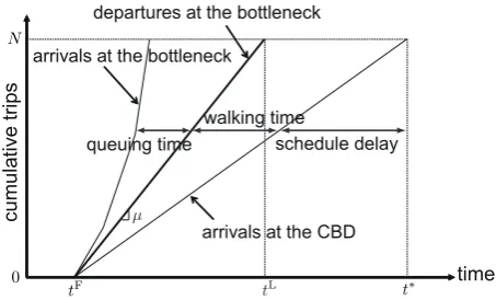
N∗_{(t) is given by}

N∗(t)=µ(t−tF) (9)

as illustrated in Figure 2. Thus, the commuting cost (4) of commutersican be rewritten as

ˆ

ci(t)=αiq(t)−fi(t−tF)+βi(t∗−tF), (10)

where fiis defined as

fi=βi−(λi−βi) wµ

d >0. (11)

This leads to the following proposition that characterizes the equilibrium number ˆn∗(t)=[ ˆn∗

i(t)]

Proposition 1. The equilibrium distributionnˆ∗(t)of trip timing coincides with the solution of the following

linear programming problem:

min

ˆ n_(t)

∑

i∈I

∫

1

αi {

−fi(τ−tF)+βi(t∗−tF) }

ˆ

ni(τ) dτ (12a)

s.t. ∑ i∈I

ˆ

ni(t)≤µ ∀t∈R, ∫

ˆ

ni(t) dt=Ni ∀i∈ I, niˆ(t)≥0 ∀i∈ I, ∀t∈R. (12b)

Proof. See Appendix B □

Let us define the (travel) time-based cost as the cost converted into equivalent travel time. Then, since the time-based cost of a commuteriis given by the cost divided byαi, we can say

that{−fi(t−tF_)+β

i(t∗−tF)}/αirepresents the sum of thetime-basedschedule delay cost and the time-basedwalking time cost of a commuter i who travels at timet. Therefore, Proposition 1 indicates that at the equilibrium, the sum of the totaltime-basedschedule delay cost and the total

time-basedwalking time cost is minimized, but the sum of total schedule delay cost and walking time cost is not necessarily minimized.9

The condition (6a) shows that the commuting cost ˆci(t) of a commuteriis minimized att∈Sˆi,

and thus, we have

        

ˆ

ci(ti)≤cˆi(tj)

ˆ

cj(tj)≤cˆj(ti)

∀ti∈Sˆi, ∀tj∈Sˆj, ∀i,j∈ I. (13)

This leads to the following condition:

ˆ

ci(ti)

αi

+cˆj(tj)

αj

≤ cˆi(tj)

αi

+ cˆj(ti)

αj

∀ti∈Sˆi, ∀tj∈Sˆj, ∀i,j∈ I. (14)

Substituting (10) into this, we have the condition that characterizes the distribution of trip timing:

( fi αi

− fj

αi )

(ti−tj)≥0 ∀ti∈Sˆi, ∀tj∈Sˆj, ∀i,j∈ I. (15)

This condition indicates thatcommuters depart the bottleneck (arrive the CBD) in order of increasing fi/αi. This implies that−fi/αi represents the incentive for a commuteri to be an “early bird”

(i.e., to arrive at work earlier than other commuters) and that competition for parking creates commuters’ early-bird incentives because d(−fi/αi)/dd>0. Furthermore, when fi/αi< fj/αj, the

parking location of a commuterimust be (weakly) closer to the CBD than that of a commuterj. Therefore, commuters with highλido not necessarily park close to the CBD.

We next investigate the properties of the equilibrium commuting cost [c∗

i]. For this, we suppose

in this section that fi−1/αi−1 ≤ fi/αifor alli∈ I\{1}without loss of generality, and considerti−1,i

such thatti−1,i ∈Sˆi−1∩Sˆi.10 Then, the difference in the time-based equilibrium commuting cost

9_{It is noteworthy that the sum of the total schedule delay cost and total walking time cost is minimized at the}

equilibrium if we consider homogeneous commuters.

10_{It follows from Lemma 1 and (15) that for anyi∈ I\{1}, there exists a value ofti}

between commutersi−1 andiis given by c∗ i αi − c ∗

i−1 αi−1

=

( βi αi

−βi−1

αi−1 )

(t∗_−tF₎₋ (

fi αi

− fi−1

αi−1 )

(ti−1,i−tF) ∀i∈ I\{1}, (16a)

ti−1,i=tF+

∑i−1

k=1Nk

µ . (16b)

This shows that the values of fi/αi,βi/αi, andNi/µdetermine the sign of the differencec∗_i/αi− c∗

i−1/αi−1. For example, if βi−1/αi−1 ≥ βi/αi for all i ∈ I\{1}, then the time-based equilibrium

commuting cost of a commuteri−1 is higher than that of a commuteri, i.e., a commuter traveling earlier incurs a higher time-based commuting cost. It is noteworthy that this property cannot be observed in the standard bottleneck model. In fact, when we consider the case without parking congestion (i.e.,d→ ∞), (16a) is rewritten as

lim

d→∞

{_c∗

i αi

− c

∗

i−1 αi−1

}

=

( βi αi

− βi−1

αi−1

) ∑I

k=iNk

µ . (17)

Because limd→∞fi=βi, this shows that in the standard bottleneck model, a commuter traveling

later incurs a higher time-based commuting cost.

We consider the effects of the expansion of the parking capacityd on the equilibrium com-muting cost. It follows from (16b) that at the equilibrium, the travel time costαiq(t), the schedule

delay costβi(t∗−aˆ(t)), and the walking time costλiwl(t) of a commuteriare expressed as

αiq(t)=αi i ∑

k=1 ( fk αk − fi αi ) Nk µ +βi

(

1+wµ

d

)∑

k∈INk

µ , (18a)

βi(t∗−aˆ(t))=βi (

1+wµ

d )       

t∗−t−w

d ∑ k∈I Nk        , (18b)

λiwl(t)=λi wµ

d

{₍

1+wµ

d

)∑

k∈INk µ −(t

∗_−t)

}

. (18c)

Differentiating these costs with respect tod, we have

d{αiq(t)}

dd = wµ d2        αi i ∑

k=1 (

λk−βk αk

−λi−βi

αi )

Nk µ −βi

∑ k∈INk

µ        , (19a)

d{βi(t∗−aˆ(t))}

dd =βi wµ d2       

t+w

d ∑

k∈I

Nk−tF       

>0, (19b)

d{λiwl(t)}

dd =−λi wµ d2       

t+w

d ∑

k∈I

Nk−tF       

<0. (19c)

given by

c∗_i =_βi

(

1+wµ

d

)∑

k∈INk µ −αi

i ∑

k=1 (

fi αi

− fk

αk )

Nk

µ , (20a)

TC∗=∑

i∈I

βiNi (

1+wµ

d

)∑

k∈INk

µ −

∑

i∈I

αiNi i ∑

k=1 (

fi αi

− fk

αk )

Nk

µ . (20b)

In fact, we can easily see that such a situation actually exists by differentiatingTC∗_{with respect}

tod.

The results obtained above can be summarized as follows:

Proposition 2. The equilibrium distribution of trip timing has the following properties:

(a) Commuters with smaller fi/αitravel earlier and park closer to the CBD.

(b) Suppose without loss of generality that fi−1/αi−1≤ fi/αifor all i∈ I\{1}. Then, the difference in the equilibrium time-based commuting cost between commuters i−1and i is expressed as

c∗

i αi

− c

∗

i−1 αi−1

=

( βi αi

− βi−1

αi−1 )

(t∗−tF)−

( fi αi

− fi−1

αi−1 )

(ti−1,i−tF) ∀i∈ I\{1}. (21)

4

Social optimum

This section characterizes the optimal distribution of trip timing and parking locations. We define the social optimum as a state wherein the total commuting cost is minimized. The total commuting costTC(n(t,l)) is represented as a function of the numbern(t,l)=[n_i(t,l)] of commuters who travel

at timetand park at locationl, which we call distribution of trip timing and parking locations:

TC(n(t,l))= ∑

i∈I "

ci(τ, ℓ)ni(τ, ℓ) dτdℓ. (22)

Therefore, the optimal distribution of trip timing and parking locations coincides with a solution to the following problem:

min

n(t,l)

TC(n(t,l)) (23a)

s.t. ∑

i∈I

∫

ni(t,l) dl≤µ ∀t∈R, ∑

i∈I

∫

ni(t,l) dt≤d ∀l∈R+, (23b)

"

ni(t,l) dtdl=Ni ∀i∈ I, ni(t,l)≥0 ∀i∈ I, ∀t∈R,∀l∈R+. (23c)

Because the queue at the bottleneck is completely eliminated at the social optimum as proved in the studies involving standard bottleneck models, the total commuting cost can be rewritten as

TC(n(t,l))= "

{

λiwℓ+βi{t∗−a(τ, ℓ)} }

ni(τ, ℓ) dτdℓ (24)

The Karush–Kuhn–Tucker (KKT) conditions of this problem are given by

         co

i(t,l)=coi if noi(t,l)>0 co

i(t,l)≥coi if noi(t,l)=0

∀i∈ I, ∀t∈R, ∀l∈R+, (25a)

        

∑ i∈I

∫ no

i(t,l) dl=µ if pq(t)>0 ∑

i∈I

∫ no

i(t,l) dl≤µ if pq(t)=0

∀t∈R, (25b)

        

∑ i∈I

∫ no

i(t,l) dt=d if pp(l)>0 ∑

i∈I

∫ no

i(t,l) dt≤d if pp(l)=0

∀l∈R+, (25c)

"

no_i(t,l) dtdl=Ni ∀i∈ I. (25d)

wherepq(t),pp(l), andco_i are the Lagrange multipliers for the first, second, and third constraints of (23), respectively, andco

i(t,l) is defined as

co_i(t,l)=λiwl+βi{t∗−a(t,l)}+pq(t)+pp(l). (26)

LetSo

i ={(t,l)∈R×R+|coi(t,l)=coi}. Then, the condition (25a) leads to the following condition:

for any (ti,li),(˜ti,li˜)∈ So

i such thatti<˜ti,

Substituting (26) into this condition, we obtain

         co

i(ti,li)+coi(˜ti,li˜)=coi(ti,˜li)+coi(˜ti,li) if a(˜ti,li)≤t

∗

co

i(ti,li)+coi(˜ti,li˜)<coi(ti,˜li)+coi(˜ti,li) if a(˜ti,li)>t

∗ ∀(ti,li),(˜ti,

˜

li)∈ So_i, ∀i∈ I. (28)

The condition (28) characterizes the distributionno_i(t,l) of trip timing and parking locations for commutersi. The first condition shows the existence of a situation wherein the total commuting cost does not change even if commutersichange their trip timing and/or parking location, i.e., the optimal distribution is not uniquely determined. The second condition indicates that a commuter

iwho travels later tends to park closer to the CBD as a late arrival incurs prohibitive cost. This property is quite different from that at the equilibrium.

Condition (25a) also gives us the condition that the commuting costs of commutersiand j

satisfy

         co

i(ti,li)+coj(tj,lj)≤coi(tj,li)+coj(ti,lj) co

i(ti,li)+coj(tj,lj)≤coi(ti,lj)+coj(tj,li)

∀(ti,tj)∈ Soi,∀(tj,lj)∈ Soj,∀i,j∈ I. (29)

Substituting (26) into this condition, we have the following lemma.

Lemma 2. For any i,j∈ I,(ti,li)∈ So_i, and(tj,lj)∈ So_j, the following conditions are satisfied.

(a) The trip timing tiand tjsatisfy

              

(βi−βj)(ti−tj)≥0 if a(ti,lj)≤t∗, a(tj,li)≤t∗,

ti<tj if a(ti,lj)≤t∗, a(tj,li)>t∗, ti>tj if a(ti,lj)>t∗, a(tj,li)≤t∗.

(30)

(b) Ifλi−βi≥λj−βj, then li≤lj.

Proof. See Appendix C. □

This lemma shows the properties of the optimal distributionno(t,l) of trip timing and parking

locations. The condition (30) suggests that during time interval [tF_,t∗_−wlC

max], commuters travel

in order of increasingβi, wherelCmaxis the closest parking location of commuters with the greatest βi. In the time interval [t∗−wlCmax,t∗], commuters who parkl <lCmaxtravel. This result sharply

contrasts to the equilibrium case, in which commuters park in order of increasing distance from the CBD (i.e., park outwards).

Lemma 2 (b) shows that a commuter with largerλi−βiparks closer to the CBD at the social

optimum. This implies that a commuter’s parking location is affected not only by the value of walking timeλibut also by the value of schedule delayβi. Therefore, commuters with high value

of walking time may not park close to the CBD if their value of schedule delay is high. The following proposition summarizes these results.

(a) For any i∈ Iand(ti,li),(˜ti,l˜i)∈ So_i such that ti≤t˜i,

         co

i(ti,li)+coi(˜ti,l˜i)=coi(ti,l˜i)+coi(˜ti,li) if a(˜ti,li)≤t

∗_,

co

i(ti,li)+coi(˜ti,l˜i)<coi(ti,l˜i)+coi(˜ti,li) if a(˜ti,li)>t

∗_. (31)

(b) For any i,j∈ I,(ti,li)∈ So_i, and(tj,lj)∈ So_jsuch that ti≤tj,

{

βi≤βj and a(tj,li)≤t∗ }

or tj+li>t∗, (32a) {

(λi−βi)−(λj−βj) }

(li−lj)≤0. (32b)

5

E

ff

ects of parking fees and congestion tolls

In the previous section, we show that the equilibrium distribution of trip timing and parking locations does not coincide with the optimal one. This is because at the equilibrium, commuters will park outwards and queuing congestion occurs. This implies that the introduction of parking fees and congestion tolls may improve the commuting cost of commuters. Therefore, this section examines the effectiveness of such policies.

5.1

Parking fees

We first consider the situation in which the planner imposes a location-dependent parking fee

pp_{(l) to equalize demand for parking at locationlwith supplyd(i.e., a competitive parking fee).}

We assume that under this policy, commuters can choose their parking location before their trip. The commuting cost of a commuteriwho travels at timetand parks at locationlis then expressed as

cp_i(t,l)=pp_(l)+c i(t,l)

=pp(l)+_αiq(t)+_λiwl+_βi{t∗−a(t,l)}., (33)

Since the parking feepp_{(l) equalizes demand and supply for parking at locationl, the equilibrium}

conditions are given by

        

cp_i(t,l)=c_ip∗ if np_i(t,l)>0

cp_i(t,l)≥cp_i∗ if np_i(t,l)=0 ∀i∈ I, ∀t∈R, ∀l∈R

+, (34a)

        

∑ i∈I

∫

np_i(t,l) dl=µ if q(t)>0

∑ i∈I

∫

np_i(t,l) dl≤µ if q(t)=0 ∀t∈R, (34b)

        

∑ i∈I

∫

np_i(t,l) dt=d if pp_(l)>0 ∑

i∈I

∫

np_i(t,l) dt≤d if pp(l)=0 ∀l∈R

+, (34c)

"

np_i(t,l) dtdl=Ni ∀i∈ I. (34d)

Condition (34a) is the no-arbitrage condition for commuters’ choice of trip timing and park-ing location. (34b) and (34c) represent the capacity constraints of the bottleneck and parkpark-ing, respectively. Note that (34c) can be interpreted as the market clearing condition. In fact, this condition suggests that if demand∑

i∈I

∫

ni(t,l)dtfor parking at locationlequals the supplyd,

thenpp(l)≥0. Condition (34d) is conservation law of the population. LetSp_i ={(t,l)∈R×R+|cp_i(t,l)=cp

∗

i }. Then, (34a) gives us the following conditions onnp(t,l):

for anyi∈ I, (ti,li),(˜ti,l˜i)∈ Sp_i such thatti<t˜i,

Substituting (33) into (35), we obtain

        

cp_i(ti,li)+c_ip(˜ti,li˜)=cp_i(ti,li˜)+cp_i(˜ti,li) if a(˜ti,li)≤t∗

cp_i(ti,li)+cp_i(˜ti,li˜)<cp_i(ti,li˜)+cp_i(˜ti,li) if a(˜ti,li)>t∗ ∀(ti,li),(˜ti,

˜

li)∈ Sp_i, ∀i∈ I. (36)

These conditions coincide with (28), which implies that the properties of the equilibrium distri-butionnp_i(t,l) of trip timing and parking locations of commutersiare the same as those at the social optimum.

Condition (34a) also gives the following conditions that should be satisfied at the equilibrium with the existence of parking fees:

            

cp_i(ti,li) αi

+c

p j(tj,lj)

αj

≤ c

p i(tj,li)

αi

+c

p j(ti,lj)

αj

cp_i(ti,li)+cp_j(tj,lj)≤cp_i(ti,lj)+cp_j(tj,li)

∀(ti,li)∈ Sp_i, ∀(tj,lj)∈ Sp_j, ∀i,j∈ I, (37)

Substituting (33) into (37) yields the following lemma.

Lemma 3. For any i,j∈ I,(ti,li)∈ Sp_i, and(tj,lj)∈ Sp_j, the following conditions hold at the equilibrium

with the existence of parking fees:

(a) The trip timings tiand tjsatisfy

                 (

βi αi−

βj αj )

(ti−tj)≥0 if a(ti,lj)≤t∗, a(tj,li)≤t∗,

ti<tj if a(ti,lj)≤t∗_{, a(tj,li)>t}∗_,

ti>tj if a(ti,lj)>t∗_{, a(tj,li)≤t}∗_.

(38)

(b) Ifλi−βi≥λj−βj, then li≤lj.

Proof. Similar to the proof of Lemma 2. □

This lemma characterizes the equilibrium distribution of trip timing and parking locations with the existence of parking fees. Lemma 3 (a) shows that commuters with smallerβi/αitravel

earlier during the time interval [tF,t∗−wlC_max] and that commuters parking atl ≤ lC_max travel during [t∗_−wlC

max,t∗], wherelCmaxis the closest parking location for commuters with the greatest βi/αi. Therefore, in general, the optimal distribution of trip timing cannot be achieved only by

imposing a parking fee. In contrast, Lemma 3 (b) coincides with Lemma 2 (b), which implies that the existence of parking fees leads to the optimal distribution of parking locations.11

In order to investigate the properties of the equilibrium commuting costcp_i∗, we consider the equilibrium trip costτp_i∗and equilibrium parking costρp_i∗, which are defined as

cp_i∗=τp_i∗+ρp_i∗, (39a)

τp_i∗=αiq(ti)+βi(t∗−ti), (39b)

ρp_i∗=pp(li)+(λi−βi)wli, (39c)

where (ti,li)∈ Sp_i. By usingtijsuch that (tij,li)∈ Sp_i and (tij,lj)∈ Sp_j andlijsuch that (ti,lij)∈ Sp_i

and (tj,lij)∈ Sp_j, we have

τp_i∗ αi

−τ

p∗

j αj

=

( βi αi

−βj

αj )

(t∗−tij). (40a)

ρp_i∗−ρp_j∗={(λi−βi)−(λj−βj) }

wlij. (40b)

(40a) shows that ifβi/αi> βj/αj, thenτp

∗

i /αi≥τ p∗

j /αj. That is, a commuter traveling later incurs a

higher time-based equilibrium trip cost. (40b) indicates that a commuter who parks closer to the CBD incurs a higher equilibrium parking cost.

The results obtained above are summarized as follows.

Proposition 4. The equilibrium distributionnp(t,l)=[np

i(t,l)]of trip timing and parking locations, the equilibrium trip cost[τp_i∗], and the equilibrium parking cost[ρp_i∗]with the existence of parking fees satisfy the following conditions:

(a) For any i∈ I,(ti,li),(˜ti,li˜)∈ Sp_i such that ti<ti,˜

        

cp_i(ti,li)+cp_i(˜ti,l˜i)=cp_i(ti,l˜i)+cp_i(˜ti,li) if a(˜ti,li)≤t∗,

cp_i(ti,li)+cp_i(˜ti,l˜i)<cp_i(ti,l˜i)+cp_i(˜ti,li) if a(˜ti,li)>t∗.

(41)

(b) For any i,j∈ I,(ti,li)∈ Sp_i, and(tj,lj)∈ Sp_j such that ti≤tj,

{ βi αi

≤ βj

αj

and a(tj,li)≤t∗ }

or tj+li>t∗, (42a)

{

(λi−βi)−(λj−βj) }

(li−lj)≤0. (42b)

(c) A commuter traveling later incurs a higher equilibrium time-based trip cost.

(d) A commuter parking closer to the CBD incurs a higher equilibrium parking cost.

This proposition suggests that the optimal distribution of parking locations is achieved by introducing parking fees. However, we should note that because βi/αi > fi/αi for all i ∈ I,

this policy reduces the early-bird incentives for all commuters. This may lead to a temporal concentration of traffic demand, thereby exacerbating the bottleneck congestion. In Section 6, we will observe that such a situation actually exists. This fact suggests that parking policies may in fact exacerbate traffic congestion and should be implemented along with a measure aimed to alleviate peak congestion.

5.2

Congestion tolls

We next examine the effects of a time-varying congestion tollpq_{(t). This toll p}q_{(t) completely}

eliminates the bottleneck congestion12 but does not affect commuters’ parking location prefer-ences. Thus, under this policy, commuters park outwards. It is noteworthy that since we consider

12_{Note that the tradable bottleneck permits proposed by Akamatsu (2007) and Wada and Akamatsu (2013) have the}

heterogeneous commuters, the congestion tollpq_{(t) does not equal the travel time costα} iq(t) at

the equilibrium without pricing policies and is set so that the travel demand∑

i∈Inˆi(t) equals the

supply (capacity)µ. Therefore, the equilibrium is defined as a state that satisfies the following conditions:

        

ˆ

cq_i(t)=c_iq∗ if nˆq_i(t)>0

ˆ

cq_i(t)≥cq_i∗ if nˆ_iq(t)=0 ∀i∈ I, ∀t∈R, (43a)

         ∑

i∈Inˆ

q

i(t)=µ if pq(t)>0 ∑

i∈Inˆ

q

i(t)≤µ if pq(t)=0

∀t∈R, (43b)

∫

ˆ

nq_i(t) dt=Ni ∀i∈ I, (43c)

where ˆcq_i(t) is the commuting cost of a commuteritraveling at timet, which is given by

ˆ

cq_i(t)=pq(t)+λi wµ

d (t−t F_)+β

i{t∗−aˆ(t)}. (44)

cq_i∗denotes the equilibrium commuting cost under the congestion toll.

Condition (43a) is the no-arbitrage condition for commuters’ trip timing choices. (43b) denotes the bottleneck capacity constraints, which ensure that the bottleneck congestion is completely eliminated at the equilibrium. Condition (43c) provides the flow conservation for commuting demand.

We can easily show that equilibrium conditions (43) are equivalent to the following optimiza-tion problem:

Proposition 5. The equilibrium distributionnˆq(t)=[ ˆnq

i(t)]of trip timing with the existence of congestion tolls coincides with the solution of the following linear programming problem:

min

ˆ n(t)

∑

i∈I

∫ _{

λi wµ

d (τ−t F_)+β

i{t∗−aˆ(τ)} }

ˆ

ni(τ) dτ (45a)

s.t. ∑ i∈I

ˆ

ni(t)≤µ ∀t∈R, ∫

ˆ

ni(t) dt=Ni ∀i∈ I, nˆi(t)≥0 ∀i∈ I, ∀t∈R. (45b)

Proof. Similar to the proof of Proposition 1. □

This proposition suggests that the sum of total schedule delay cost and total walking time cost, which equals the total commuting cost minus total toll revenue, is minimized at the equilibrium. Hence, the congestion toll achieves the social optimum under condition (2) (i.e., parking spaces are occupied in strict order from the CBD). Furthermore, by comparing Propositions 1 and 5, we can see that commuters with largeαi(rich commuters) will gain a great deal from the congestion

toll, but commuters with smallαi(poor commuters) may lose.

Let ˆSq_i ={t∈R|cˆq_i(t)=cq_i∗}. Then, as in Section 3, condition (43a) gives the following condition that is satisfied at the equilibrium with the existence of congestion tolls:

ˆ

Substituting (44) into (46), we have

( fi−fj

)

(ti−tj)≥0 ∀ti∈Sˆq_i, ∀tj∈Sˆq_j, ∀i,j∈ I. (47)

This condition shows that commuters travel in order of increasing fiand that the value of the

travel timeαi does not affect the equilibrium distribution ˆnq(t) of trip timing. Furthermore,

since commuters park outwards in this case, the congestion toll cannot significantly improve the distribution of parking locations.

We suppose in this section that fi−1≤ fifor alli∈ I\{1}without loss of generality. Then, by

usingti−1,isuch thatti−1,i∈Sˆq_i−1∩Sˆ q

i, we can easily show that the equilibrium commuting costc q∗

i

satisfies

cq_i∗−cq_i−∗₁=(

βi−βi−1)(t∗−tF)−(fi− fi−1)(ti−1,i−tF), (48a)

ti−1,i=tF+

∑i−1

k=1Nk

µ , (48b)

tF=t∗−

(

1+wµ

d

)∑

k∈INk

µ . (48c)

This implies that similar to the equilibrium with no pricing policies, the values of fi, βi, and Nı/µ determine the sign of the difference cq_i∗−c_iq₋∗₁. Hence, ifβi−1 ≥ βi for all i ∈ I\{1}, then

the equilibrium commuting cost of a commuteri−1 is higher than that of a commuteri, i.e., a commuter who travels earlier incurs a higher commuting cost.

The equilibrium commuting costcq_i∗of a commuteriis obtained from (48) as

cq_i∗=βi (

1+wµ

d

)∑

k∈INk

µ −

i ∑

k=1 (

fi− fk) Nk

µ . (49)

Therefore, iffi−1/αi−1≥ fi/αi(i.e.,αi−1≤αi) for alli∈ I\{1}, we have

cq_i∗−c∗_i =_αi

I ∑

k=i (

fi αi

− fk

αk ) Nk µ − i ∑

k=1

(fi− fk) Nk

µ . (50)

This indicates that a value ofiq _{∈ I\{1}exists such thatc}q∗

k −c

∗

k ≥0 for allk∈ {1,· · ·,iq−1}and cq_k∗−c∗

k≤0 for allk∈ {iq,· · · ,I}, which implies that rich commuters gain but poor commuters lose

from the imposition of a congestion toll.

The total commuting costTCq_{and the total toll revenueP}q_{are obtained as}

TCq=∑

i∈I       

βiNi (

1+wµ

d

)∑

k∈INk

µ −Ni

i ∑

k=1

(fi−fk) Nk µ        , (51a)

Pq=∑

i∈I Ni        i ∑

k=1 fk

Nk µ − fi

Ni 2µ        . (51b)

This shows that the expansion of the parking capacitydmay increase the total commuting cost

TCq_{but must decreaseTC}q_−Pq_{. That is, the expansion of the parking capacity reduces the total}

commuting cost if the planner redistributes the toll revenue.

Proposition 6. The equilibrium distribution of trip timing with the existence of congestion tolls has the following properties:

(a) Commuters with smaller fitravel earlier and park closer to the CBD.

(b) Suppose without loss of generality that fi−1 ≤ fi for all i ∈ I\{1}. Then, the difference in the equilibrium time-based commuting cost between commuters i−1and i is expressed as

cq_i∗−cq_i−∗₁=(

βi−βi−1)(t∗−tF)−(fi− fi−1)(ti−1,i−tF) ∀i∈ I\{1}. (52)

(c) If the planner redistributes the toll revenue, the expansion of the parking capacity d must decrease the total commuting cost; otherwise, the expansion may increase the total commuting cost.

5.3

Combination of parking fees and congestion tolls

We finally consider the effects of introducing parking fees and congestion tolls. In this case, the distributionnpq(t,l)=[npq

i (t,l)] of trip timing and parking locations, the congestion tollpq(t), the

parking feepp_{(l), and the commuting costc}pq

i at the equilibrium are obtained from the following

conditions:

        

cpq_i (t,l)=c_ipq∗ if npq_i (t,l)>0

c_ipq(t,l)≥c_ipq∗ if npq_i (t,l)=0 ∀i∈ I, ∀t∈R, ∀l∈R+, (53a)

        

∑ i∈I

∫

npq_i (t,l) dl=µ if pq_(t)>0 ∑

i∈I

∫

npq_i (t,l) dl≤µ if pq_(t)=0 ∀t∈R, (53b) 

       

∑ i∈I

∫

npq_i (t,l) dt=d if pp_(l)>0 ∑

i∈I

∫

npq_i (t,l) dt≤d if pp_(l)=0 ∀l∈R+, (53c)

"

npq_i (t,l) dtdl=Ni ∀i∈ I, (53d)

wherecpq_i (t,l) is the commuting cost of a commuteriwho travels at timetand parks at locationl

cpq_i (t,l)=pq(t)+pp(l)+λiwl+βi{t∗−a(t,l)}. (54)

Because conditions (53) coincide with (25), the optimal distribution of trip timing and parking locations is achieved by introducing parking fees and congestion tolls.

LetSpq_i ={(t,l)∈ R×R+| cpq_i (t,l)=cpq_i ∗}. We then examine the properties of the equilibrium trip costτpq_i ∗and equilibrium parking costρpq_i ∗, which are defined as

cpq_i ∗=_τpq∗

i +ρ pq∗

i , (55a)

τpq_i ∗=pq(ti)+βi(t∗−ti), (55b)

ρpq_i ∗=pp(li)+(λi−βi)wli, (55c)

and (tj,lij)∈ Spq_j , we haveτpq

∗

i −τ pq∗

j andρ pq∗

i −ρ pq∗

j as follows

τpq_i ∗−τpq_j ∗=(_βi−βj )

(t∗−tij). (56a)

ρpq_i ∗−ρpq_j ∗={(λi−βi)−(λj−βj) }

wlij. (56b)

Condition (56a) shows that a commuter traveling later incurs a higher time-based equilibrium trip cost. Condition (56b) indicates that a commuter who parks closer to the CBD incurs a higher equilibrium parking cost.

These results establish the following proposition.

Proposition 7. The equilibrium distribution of trip timing and parking locations, the equilibrium trip

cost[τpq_i ∗], and the equilibrium parking cost[ρpq_i ∗]with the existence of parking fees and congestion tolls have the following properties.

(a) The equilibrium distribution of trip timing and parking locations coincides with the optimal one.

(b) A commuter traveling later incurs a higher equilibrium trip cost.

(c) A commuter parking closer to the CBD incurs a higher equilibrium parking cost.

The effects of the parking fee and congestion toll on the distribution of trip timing and parking locations are summarized in Table 1. The results obtained in this section demonstrate that introducing pricing policies significantly changes the distribution of trip timing and parking locations, thereby leading to complex changes in commuters’ commuting costs. As an example, we consider a case where for alli∈ I\{1},

fi−1> fi, βi−1> βi, λi−1−βi−1> λi−βi, αi−1 > αi, (57a) fi−1

αi−1 < fi

αi , βi−1

αi−1 < βi

αi

, λi−1−βi−1 αi−1

< λi−βi αi

. (57b)

That is, commuters with smaller (larger)iare rich (poor). In this case, Propositions 2, 4, 6, and 7 give us the difference in the commuting costs between commutersi−1 andifor alli∈ I\{1}as

c∗

i αi

> c

∗

i−1 αi−1

, (58a)

τp_i∗ αi

> τ p∗

i−1 αi−1

, ρp_i∗< ρp_i−∗₁, (58b)

cq_i∗<cq_i−∗₁, (58c)

τpq_i ∗< τpq_i−∗₁, ρp_i∗< ρp_i−∗₁. (58d)

This shows that the effect of each pricing policy on each type of commuter can differ quite radi-cally. Hence, the planner should understand these mechanisms to ensure that any implemented road/parking policy will be effective.

Table 1: Equilibrium distribution of trip timing and parking locations with/without policies

policy the order of trip timing the order of parking location no-pricing policies ascending order of fi/αi ascending order of fi/αi

parking fee ascending order ofβi/αi* descending order ofλi−βi

congestion toll ascending order of fi ascending order of fi

parking fee+congestion toll ascending order ofβi* descending order ofλi−βi

*t∈[tF_,t∗_−wlC max]

(1965), Keeler and Small (1977), Arnott et al. (1993), Arnott and Kraus (1995), Yang and Meng (2002), Akamatsu (2007), and Verhoef (2007).

We consider that the planner chooses a parking and bottleneck capacity, d andµ, so as to minimize the social cost, which is defined as the sum of the total commuting costTC(n(t,l))

defined in (24), parking capacity costKp_{(d), and bottleneck capacity costK}q_{(µ). Therefore, the}

optimal parking and bottleneck capacity,do_andµo_{, is obtained from the following problem:}

min

n(t_,l)_,d_,µ

TC(n(t,l))+Kp(d)+Kq(µ) s.t. (23b),(23c). (59)

The capacity costsKp(d) andKq(µ) are assumed to be homogeneous of degree one ind andµ, respectively.

The KKT conditions of this problem are given by (25) and the following two conditions

              

dKq(µ) dµ −

∫

pq(τ)dτ=0 if µ >0,

dKq(µ) dµ −

∫

pq(τ)dτ≥0 if µ=0,

(60a)

            

dKp_(d)

dd − ∫

pp(ℓ)dℓ=0 if d>0,

dKp_(d)

dd − ∫

pq(τ)dℓ≥0 if d=0.

(60b)

SinceKq_{(µ) andK}p_{(d) are homogeneous of degree 1, the conditions (60) yield}

Kq(µo)=µo ∫

pq(t)dt, (61a)

Kp(do)=do ∫

pp(l)dl. (61b)

This leads to the following proposition.

Proposition 8. Suppose that the parking and bottleneck capacity costs, Kp_{(d)and K}q_{(µ), are homogeneous}

of degree one in d andµ, respectively. Then, parking fee revenues equal the cost Kp(do)for the optimal parking capacity do_{, and congestion toll revenues equal the cost K}q_(µo_{)for the optimal bottleneck capacity} µo.

6

A simple example

This section analyzes the model in a simple setting to show concretely properties of equilibrium and effects of pricing policies. We assume that commuters are divided in two groups (i.e.,I=2) and thatN1=N2=N/2. In addition, the parametersαi,βi,λiare assumed to satisfy

f1 α1 <

f2 α2,

β1 α1 <

β2 α2,

λ1−β1 α1 <

λ2−β2

α2 , (62a)

f1> f2, β1> β2, λ1−β1> λ2−β2. (62b)

Note that this assumption gives

α1> α2, λ1> λ2, β1−β2> f1− f2. (63)

Both (62) and (63) imply that commuters 1 and 2 can be considered rich and poor commuters, respectively.

6.1

Equilibrium with no pricing policies

We first consider a situation in which neither parking fees nor congestion tolls are imposed. Let

tF

i andtLi be the first and last trip timing of commutersi, respectively. Then, Proposition 2 and

(62) givestF

i andtLi as follows:

tF₁ =tF=t∗−

(

1+wµ

d

)_N

µ, t

L

1 =tF2 =t

∗₋w

dN− N

2µ, t L

2 =tL =t

∗₋w

dN. (64)

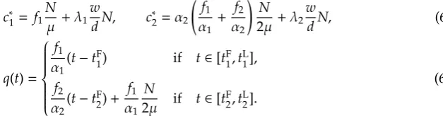
It follows from (6a) and this that the equilibrium commuting costc∗

i and queuing timeq(t) are

obtained as

c∗₁= f1 N

µ +λ1 w

dN, c

∗

2=α2 (

f1 α1

+ f2

α2 )

N

2µ+λ2 w

dN, (65a)

q(t)=

               f1 α1(

t−tF

1) if t∈[tF1,tL1], f2

α2(t

−tF₂)+ f1

α1 N

2µ if t∈[t F 2,tL2].

(65b)

Figure 3 illustrates the queuing timeq(t). Thus, total queuing timeQ∗_{and total commuting cost}

TC∗_{at the equilibrium are given by}

Q∗=

[ 3 f1 α1 + f2 α2 ] N2

8µ, (66a)

TC∗=

[(

2+α2

α1 )

f1+ f2+2 (λ1+λ2) wµ

d

]_N2

4µ. (66b)

Differentiating (65) and (66) with respect tod, we have

dc∗

1

dd =−β1 w

d2N<0, (67a)

dc∗

2

dd =

{_α

2 α1

λ1−λ2−α2 α1

β1−β2

} _w

Figure 3: Equilibrium queuing timeq(t)

dQ∗

dd = {

3λ1−β1

α1

+λ2−β2

α2 }

w

8d2N

2_{>0, (67c)}

dTC∗

dd =

{_α

2 α1

λ1−λ2− (

2+α2

α1 )

β1−β2

} _w

4d2N

2_{. (67d)}

(67) indicates that expanding parking capacitydexacerbates traffic congestion. Furthermore, if

λ1>(λ2+2β1+β2)α1/α2+β1, then expanding parking capacity also increases the total commuting

cost.

6.2

Equilibrium with parking fees

We next examine the effects of instituting parking fees. LetlC

i andlFi be the parking location for

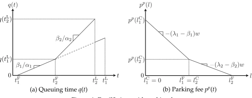
commutersiclosest to and farthest away from the CBD, respectively. Then,tF_i,t_iL,lC_i, andlF_i are obtained from Proposition 4 and (62):

tF₁=tF=t∗− N

µ, t

F 2 =t

∗₋(₁₊wµ

d

) _N

2µ, t L 2 =t

∗₋ w

2dN, t L

1 =tL =t

∗_{, (68a)}

lF₂= N

d, l

C 2 =lF1=

N

2d, l

C

1